

Abstract
The linear transform model of functional magnetic resonance imaging (fMRI) hypothesizes that fMRI responses are proportional to local average neural activity averaged over a period of time. This work reports results from three empirical tests that support this hypothesis. First, fMRI responses in human primary visual cortex (V1) depend separably on stimulus timing and stimulus contrast. Second, responses to long-duration stimuli can be predicted from responses to shorter duration stimuli. Third, the noise in the fMRI data is independent of stimulus contrast and temporal period. Although these tests can not prove the correctness of the linear transform model, they might have been used to reject the model. Because the linear transform model is consistent with our data, we proceeded to estimate the temporal fMRI impulse–response function and the underlying (presumably neural) contrast–response function of human V1.
- functional MRI
- linear systems analysis
- contrast perception
- temporal impulse–response function
- hemodynamics
- calcarine sulcus
Functional magnetic resonance imaging (fMRI) measures changes in blood oxygenation and blood volume that result from neural activity (Ogawa et al., 1990; Belliveau et al., 1992) (for review, see Moseley and Glover, 1995). Deoxygenated hemoglobin acts as an endogenous paramagnetic agent, so a reduction in the concentration of deoxygenated hemoglobin increases the T2*-weighted magnetic resonance signal.
A typical fMRI experiment measures the correlation between the fMRI response and a stimulus. From this, scientists hope to infer something about neural activity. Often it is assumed that there is a simple and direct relationship between neural activity and fMRI response, but the nature of this relationship remains unclear.
The goal of the research reported in this article is to understand how the fMRI response relates to neural activity. The vascular source of the fMRI signal places important limits on the technique. Because the hemodynamic response is sluggish, perhaps the fMRI response is proportional to the local average neural activity, averaged over a small region of the brain and averaged over a period of time. We will refer to this as the “linear transform model” of fMRI response. The linear transform model, specialized for a visual area of the brain, is depicted in Figure 1. According to this model, neural activity is a nonlinear function of the contrast of a visual stimulus, but fMRI response is a linear transform (averaged over time) of the neural activity in V1. Noise might be introduced at each stage of the process, but the effects of these individual noises can be summarized by a single noise source that is added to the output.
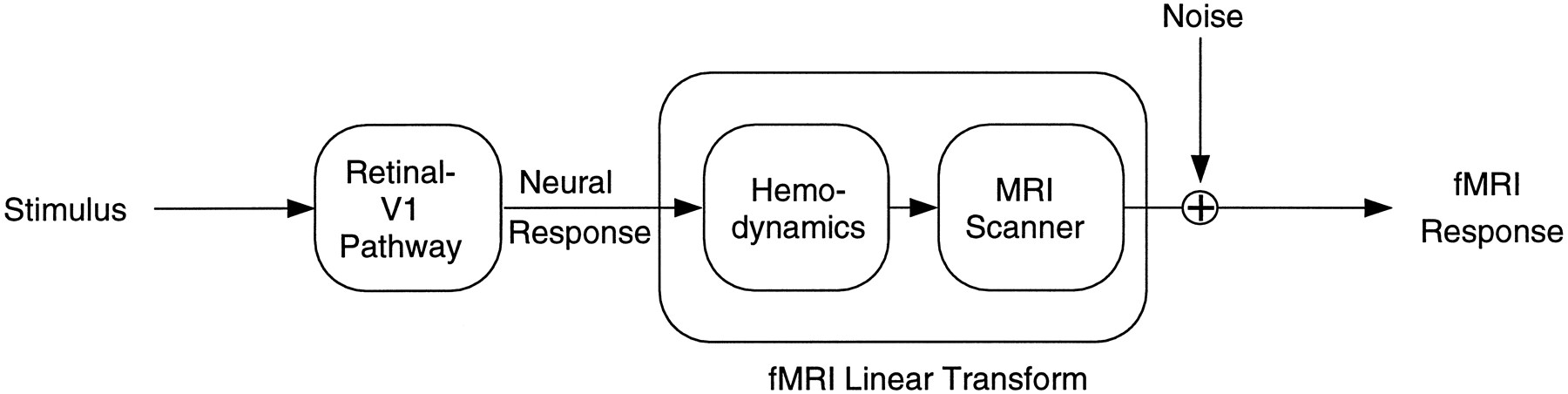
Diagram of the linear transform model. The output of the Retinal-V1 Pathway (Neural Response) is a nonlinear function of stimulus–contrast. fMRI signal, mediated byHemodynamics, is a linear transform of neural activity. That is, fMRI signal is proportional to the local average neural activity, averaged over a small region of the brain and averaged over a period of time. Noise might be introduced at each stage of the process, but the effects of these individual noises on the fMRI Response can be summarized by a single noise source.
To date, this linear transform model of fMRI response has not been tested, despite the fact that some studies rely explicitly on the linear model for their data analysis (Friston et al., 1994; Lange and Zeger, 1996). The sequence of events from neural response to fMRI response is complicated and only partially understood. It is unlikely that the complex interactions among neurons, hemodynamics, and the MR scanner would result in a precisely linear transform. However, the linear transform model might be a reasonable approximation of these complex interactions.
The linear transform model is attractive because, if it were correct, it would greatly simplify the analysis and interpretation of fMRI data. Most important, it would provide confidence in inferences made about neural activity. In addition, the relationship between neural activity and fMRI response would be characterized completely and simply by the fMRI “impulse–response function,” that is, the fMRI response resulting from a brief, spatially localized pulse of neural activity. The fMRI impulse–response function would allow one to predict the fMRI response evoked by any pattern of neural activity. This would help in experimental design, for example, in choosing the temporal duration of a visual stimulus when measuring fMRI responses in visual cortex.
According to the linear transform model, the fMRI impulse–response function would characterize completely both the spatial and the temporal averaging of the neural activity. This article concentrates on the temporal aspects of fMRI response (for a study on spatial aspects, see Engel et al., 1996). This article also concentrates only on primary visual cortex (V1), although the approach certainly may be used for studying other areas as well. Note, however, that the spatial and temporal averaging may be different in different brain areas, especially since the vasculature seems to be specialized in particular brain areas (e.g., in V1) (Zheng et al., 1991).
This article reports fMRI data from experiments designed to test the linear transform model of fMRI responses. Although these tests can not prove the correctness of the linear transform model, they might have been used to reject the model. Because the linear transform model is consistent with our data, we proceeded to estimate the temporal fMRI impulse–response function and the underlying (presumably neural) contrast–response function of human V1.
MATERIALS AND METHODS
Data acquisition. Imaging was performed on a standard clinical GE 1.5 T Signa scanner with a 5 inch surface coil. We used a T2*-sensitive gradient-recalled echo pulse sequence (TR 75 msec, TE 40 msec, flip angle 23°) with a spiral readout (Meyer et al., 1992). Inplane resolution was 2.4 × 2.4 mm, and slice thickness was 5 mm. A bite bar stabilized the subject’s head.
Each experiment consisted of a series of functional images acquired at a rate of 1.5 sec per image, as the subject viewed the stimulus. Data were collected from a single slice through the calcarine sulcus in the right hemisphere of each subject, parallel to and ∼5 mm from the medial wall. Because data were collected over several sessions, a series of anatomical axial slices was used to localize (nearly) the same slice from one session to the next. An anatomical image was taken in the same plane as the functionals preceding each experimental session. Each fMRI scan was started by hand at the stimulus onset (to within ∼0.25 sec).
Stimuli. Stimuli were presented using a Macintosh Quadra computer (Apple Computer, Cupertino, CA) and a Sanyo PLC300M LCD projector (Sanyo, Chatsworth, CA). Stimuli were focused onto a backlit projection screen inside the bore of the magnet, just above the subject’s chin. A mirror was positioned to allow the subject to view the image from the supine position. Stimuli had a mean luminance of 92 cd/m2 and subtended a visual angle of 21° vertical and 42° horizontal. The LCD projector was gamma-corrected to allow for accurate presentation of contrast stimuli.
We used two types of visual stimuli that we will refer to as “pulse” stimuli and “periodic” stimuli. Both stimuli consisted of flickering (contrast reversing with a flicker rate of 8 Hz) checkerboard patterns.
The periodic stimuli contained flickering checkerboard patterns arranged in slowly moving vertical bars (Fig.2A). As the bars moved slowly to the left, the time course of stimulation in any part of the image alternated between checks and uniform gray (Fig. 2B) with a period that we refer to as the “temporal period” of the stimulus. Note that the temporal period depends on the drift rate of the bars, and it is very different from the flicker rate (that was always fixed at 8 Hz).

Schematic of visual stimuli used in the experiments. A, One frame of the periodic stimulus consisted of vertical bars of checkerboard patternsalternating with vertical bars of uniform gray(mean). Over time, the checkerboard patterns flickered (contrast reversing with a flicker rate of 8 Hz), and the bars drifted slowly leftward. B, The time course of a single pixel of the periodic stimulus as the bars drifted. C, The time course of pixels for the pulse stimulus. Each stimulus cycle began by displaying a full-field flickering checkerboard pattern (contrast reversing at 8 Hz) for a period of time (the pulse duration). Each stimulus cycle was completed by replacing the checkerboard with uniform gray for 24 sec.
Subjects viewed periodic stimuli of various contrasts and temporal periods. The “contrast” of the stimulus is defined, in the usual way, as the maximum intensity minus the minimum, divided by twice the mean. Twenty-four periodic stimuli were viewed by each of two subjects: the stimuli had one of four temporal periods (10, 15, 30, and 45 sec) and one of six contrasts (0, 0.032, 0.063, 0.16, 0.40, and 1). The stimulus duration was fixed at 192 sec for all conditions, so the number of periodic cycles varied with the temporal period/drift rate of the stimulus. The first 12 sec (8 fMR images) of fMRI data were discarded to avoid magnetic saturation effects. The remaining 180 sec (120 images) were analyzed as described below.
Figure 2C depicts an example of the time course of a pulse stimulus. Each stimulus cycle began by displaying a full-field flickering checkerboard pattern (contrast reversing with a flicker rate of 8 Hz) for a period of time (the “pulse duration”). Each stimulus cycle was completed by replacing the checkerboard with uniform gray for 24 sec. Six cycles were repeated for each scan. Twenty-four pulse stimuli were viewed by each of two subjects: the stimuli had one of four pulse durations (3, 6, 12, and 24 sec) and one of four contrasts (0, 0.25, 0.5, and 1). The total duration of the scan depended on the pulse duration.
Analysis. Figure 3 shows how the periodic data sets were analyzed. For each condition, 120 images were acquired over 180 sec (Fig. 3A). For a given pixel, the image intensity values from all 120 fMRI images comprise a time series of data. This time series was periodic (although noisy) with a period equal to the stimulus temporal period (Fig. 3B). We measured fMRI response as the amplitude of the sinusoid that best fit the time series of each pixel. The best-fitting sinusoid was determined by computing the amplitude and phase of the appropriate component (same as the stimulus temporal period) of the discrete Fourier transform of the time series. The response amplitude was computed in this way for all pixels in the calcarine sulcus. Calcarine pixels were selected by hand from an anatomical image that was taken in the same plane as the functionals preceding each experimental session (Fig. 3C). Finally, the mean and SEM of the amplitudes were used to summarize the fMRI response (Fig. 3D).

Analysis of data for periodic stimuli.A, Sequence of fMR images. B, Time course of response at a single pixel (dashed curve) superimposed with the best-fitting sinusoid. C, Aligned anatomical image with pixels in the calcarine sulcus highlighted. D, Mean and SE of the response amplitudes of the selected pixels.
An alternate measure of fMRI signal strength is the correlation of the fMRI time course with a reference waveform such as a sinusoid. Both amplitude and correlation have been used to quantify fMRI signal strength (Bandettini et al., 1993). Amplitude and correlation are closely related; correlation is equal to amplitude divided by the total Fourier energy at all frequencies (Engel et al., 1996). In other words, the correlation measure is “normalized” with respect to the overall amplitude spectrum in the signal, including the frequency of interest. This means that two time courses that are scaled copies of one another (different amplitudes but with otherwise identical shapes) will have the same correlation coefficients. This is clearly undesirable when quantifying fMRI response as a function of stimulus strength. We therefore used the raw, “unnormalized” amplitudes.
The response amplitudes were averaged over all of the pixels in the calcarine sulcus. Also, we analyzed a subset of the data by selecting the pixels that resonated most strongly with the stimulus. Averaging over the entire calcarine sulcus has the disadvantage of including many pixels with time courses that correlate poorly with the stimulus, resulting in noisier data. Selecting a region of interest based on a measure of signal strength, however, might be misleading, given that we are trying to characterize the relationship between stimulus contrast and signal strength. Fortunately, our conclusions do not depend on which method was used for selecting the region of interest (see Discussion).
Periodic checks for head movements were made by applying an image motion estimation algorithm (Friston et al., 1996) to the functional image series. No significant head movements were discovered, presumably because the subjects were experienced and were using a bite bar.
Data from the pulse experiments were analyzed slightly differently. Pixels in the calcarine sulcus again were selected by hand from the aligned anatomical image, and the time course of the fMRI signal again was extracted for each of the selected pixels. Then the time course for each pixel was blocked with the stimulus cycle duration, and the average time course was computed, averaging across all six blocks and across all of the selected pixels.
Below, we summarize the percentage of variance in the data accounted for by various models by computing the studentized residual statistic, sometimes called the “jacknifed” residual (Atkinson, 1988). The studentized residual is the error between the measured data and the predictions (from the model) relative to the SE in the data. Specifically, the studentized residual, r, is:
 Equation 1in which pi are the predictions, di are the data points, and SEi are the standard errors. The studentized residual is an ad hoc formula for quantifying the model fits. A large value for r can be obtained either by having a very good fit (small numerator in Eq. 1) or by having very noisy data (large denominator in Eq. 1). Even so, the studentized residual is useful for comparing different models.
RESULTS
We performed three empirical tests of the linear transform model of fMRI responses. First, we tested whether fMRI responses depend separably on stimulus timing and stimulus contrast. Second, we tested whether responses to long-duration stimuli can be predicted from responses to shorter duration stimuli. Third, we tested whether the noise in the fMRI data is independent of stimulus contrast and temporal period. Because the results of these tests are consistent with the linear model, we proceeded to estimate the temporal fMRI impulse–response function and the underlying (presumably neural) contrast–response function of V1.
Time–contrast separability
The linear transform model predicts that the fMRI response should be a separable function of stimulus contrast and pulse duration (see for a formal statement and derivation of this prediction). In other words, the linear transform model holds only if the responses to pulses of different contrasts are scaled copies of one another.
The fMRI responses to the pulse stimuli for subject GMB are shown in Figure 4. Similar data were obtained from the second subject, SAE. Each curve in these figures is the time course of the fMRI response (pixel intensity) averaged across cycle repetitions and averaged across all pixels in the calcarine sulcus. The raw fMRI signal modulates ∼5–10% above and below a baseline intensity (∼90, in pixel intensity units). The curves were shifted vertically (see Parametric model), so that they asymptote at zero. The different curves correspond to different pulse durations and contrasts.

fMRI responses to pulse stimuli. Eachcurve is the mean time course of the fMRI response (pixel intensity) averaged across cycle repetitions and averaged across all pixels in the calcarine sulcus. Each panel shows data for a different pulse duration. Different curves within a panel correspond to different contrasts. The stimulus time course also is depicted in each panel. The fMRI responses increase with stimulus contrast, and the fMRI responses are blurred and delayed with respect to the time course of the stimulus. Error bars represent 1 SE.
The fMRI responses in Figure 4 increase with stimulus contrast, and the fMRI responses are blurred and delayed with respect to the time course of the stimuli. The effect of stimulus contrast is presumably attributable to increased neural activity. Since the pulse durations that were used in this experiment are rather long as compared with the time scale of neural activity in V1, the blurring and delay presumably are attributable to the hemodynamic properties of the vascular system.
The linear transform model of fMRI responses can be tested by comparing the different curves in Figure 4. The model holds only if the curves in each panel of Figure 4 are scaled copies of each other (see ). Figure 5 shows the results of the time–contrast separability test. The data points in each panel of Figure 5 are scaled copies of the data in the corresponding panel of Figure 4. The resulting scaled data seem to align without apparent significant systematic error, consistent with time–contrast separability.

Time–contrast separability test using pulse stimuli. Data in each panel are scaled copies of data in the corresponding panel of Figure 6. Error bars represent 1 SE of the scaled data. The resulting scaled data align without significant systematic error, consistent with time–contrast separability. The first principal components (solid curves) account for 86.81% of the variance in the data.
To align the curves, the three scale factors were computed using a principal components analysis to maximize the covariances between each pair of curves. The same three scale factors (one for each contrast) were used for all four pulse durations. The solid curves in each panel are the first principal components for each pulse duration. These principal component curves act as nonparametric models of the data. In particular, the first principal component is the curve that is closest (minimizing squared error) to all three scaled data sets. For subject GMB, the principal component curves account for 86.81% of the variance in the data (computed using Eq. 1). If the data for different contrasts were not scaled copies of each other, then the principal component curves would not have accounted for much of the variance. The results for subject SAE (data not shown) are very similar, and the principal component curves account for 99.01% of the variance in that data set.
The response to the lowest contrast in Figure 5(squares)shows the most scatter around the principal component. This occurs because the response to the lowest-contrast stimulus requires the largest scale factor to match the response to the full-contrast stimulus. Unscaled, each signal has about the same amount of high frequency noise (See Noise analysis). Scaling the signal amplifies the noise as well. This is reflected in the size of the error bars.
Time–contrast separability also was tested using the periodic stimuli. Figure 6 plots the fMRI response amplitude (that is, the amplitude of modulation of the response at the stimulus temporal period) as a function of stimulus contrast. fMRI response amplitude is not a linear function of stimulus contrast, but it does increase monotonically. In addition, fMRI response amplitude decreases as the temporal period shortens. The fMRI response amplitudes for zero contrast stimuli are attributable to noise.

fMRI response amplitudes for periodic stimuli as a function of stimulus contrast and temporal period for both subjects.Amplitudes are in pixel intensity units, andContrast is plotted on a logarithmic scale. Data points are mean response amplitudes (averaged over the calcarine sulcus). Error bars represent 1 SE of the mean. fMRI response amplitude increases monotonically with stimulus contrast, and it decreases as theTemporal Period shortens.
Again, the increase in response amplitude with stimulus contrast presumably is a result of increased neural activity. fMRI response is a nonlinear function of stimulus contrast, presumably because neural activity in V1 is a nonlinear function of stimulus contrast. From single-cell electrophysiological recordings, we know the response (firing rate) of neurons in V1 increases with stimulus contrast but not in proportion to stimulus contrast. For example, as the contrast is doubled from 0.5 to 1, the contrast–response of a V1 neuron typically does not double, a phenomenon known as response saturation (Maffei and Fiorentini, 1973; Dean 1981; Albrecht and Hamilton, 1982; Ohzawa et al., 1982, 1985; Sclar et al., 1990). Likewise, the fMRI response amplitudes saturate somewhat at high contrasts. (This is more easily seen in Fig. 7 by noting that the response to 100% contrast is far less than double the response to 42% contrast.) Note, however, that the nonlinearity of the fMRI contrast–response function is not a violation of the linear transform model. The linear model predicts that doubling the neural response doubles the fMRI response, but doubling the contrast does not necessarily double the neural response.

Time–contrast separability test using periodic stimuli for both subjects. Each data set is a scaled copy of the corresponding data from Figure 6, after compensating for the noise (see text). Error bars represent 1 SE of the scaled data. The curves align without significant systematic error, consistent with separability. The first principal components (solid curves) account for 99.64 and 99.01% of the variance in the data for subjects gmb andsae, respectively.
The attenuation of response amplitude for shorter temporal periods presumably is a result of temporal blurring by the hemodynamics. Although V1 neurons adapt after long-term exposure to high contrast stimuli, we certainly would not expect neurons in V1 to respondmore (that is, with higher average firing rates) to a 22.5-sec-duration flickering checkerboard than to a 5-sec-duration flickering checkerboard.
Time–contrast separability predicts that the curves in Figure 6 be scaled copies of each other. Unfortunately, because of noise in the fMRI responses, the curves do not meet at zero for zero contrast, thus violating separability. However, we can compensate for the noise (see) and demonstrate separability of the underlying (noise-free) responses.
Figure 7 shows the results of the time–contrast separability test for the periodic data sets. After compensating for the noise, the curves were scaled, as was done for the pulse data sets. The resulting data align without significant systematic error, consistent with time–contrast separability. The scale factors were determined, as before, by performing a principal components analysis of the data. The principal component curves, drawn as solid curves in Figure 7, account for 99.64 and 99.01% of the variance in the data for subjects GMB and SAE, respectively.
Pulse duration
The pulse data sets were used to perform another test of the linear transform model. According to the model, the response to a long pulse should be predictable by summing the responses to shorter pulses (see ). The pulse durations of 3, 6, 12, and 24 sec provide six predictions. For example, the response to the 6 sec pulse is predicted by summing the response to the 3 sec pulse with a copy of the same response delayed by 3 sec. The response to the 12 sec pulse is predicted by summing four shifted copies of the response to the 3 sec pulse, and so on.
Figure 8 shows the results of this analysis for the principal component curves from Figure 5. The predictions are generally consistent with the linear transform model. However, there is a systematic failure of the predictions. The responses to the shortest (3 sec) pulse tend to overestimate the responses to the longer pulses. We believe that this may be attributable to neural adaptation (see Discussion). Results for subject SAE are similar.

fMRI responses from shorter pulses can predict the responses to longer pulses. The four principal component curves (corresponding to pulse durations of 3, 6, 12, and 24 sec) from Figure5 were used to make six predictions. The predictions are generally consistent with the linear transform model. However, the responses to the shortest (3 sec) pulse tend to overestimate slightly the responses to the longer pulses.
Noise analysis
An assumption of the linear transform model is that the noise in the fMRI data is independent of stimulus contrast and stimulus temporal period. Noise amplitudes can be measured by analyzing the fMRI responses to zero contrast stimuli. Noise amplitudes also can be measured using any of the (nonzero contrast) periodic data, as long as the data is analyzed with a temporal period that is different from the stimulus temporal period. We refer to that temporal period, Ta, as the “analysis period” to distinguish it from the stimulus temporal period T.
Figure 9A plots the fMRI response amplitudes from one subject for all of our periodic stimuli. For example, the upper left graph plots response amplitude for Ta = 10, that is, the amplitude of the Fourier component of the fMRI response time course with a period of 10 sec. In each panel of Figure9A, response amplitude increases with contrast only when the analysis period is the same as the stimulus temporal period. The other curves are flat, demonstrating that the noise is, in fact, independent of both stimulus contrast and stimulus temporal period.

Noise analysis. A, fMRI response amplitudes for periodic stimuli as a function of stimulusContrast, stimulus Temporal Period, andAnalysis Period. Each panel corresponds to a different analysis period. Different curves correspond to different stimulus temporal periods. Error bars represent 1 SE. Response amplitude increases with Contrast only when the Analysis Period is the same as the stimulus Temporal Period. The other curves are measurements of the noise. The noise curves are flat, demonstrating that the noise is independent of both stimulus contrast and stimulus temporal period. B, Noise amplitudes for all periodic stimulus conditions and for all possible analysis periods. The noise is broad-band; that is, the noise amplitudes are significantly nonzero for each of the analysis periods. The solid curve, drawn for comparison, is the temporal fMRI frequency–response function, that is, the amplitude of the Fourier transform of the temporal fMRI impulse–response function (from Fig. 13).
We analyzed our data to obtain many additional noise amplitude measurements. In particular, we used a total of 60 analysis periods Ta such that: (1) Ta > 3 sec (because the sample rate of the MR scanner was 1.5 sec), and (2) 180 was an integer multiple of Ta (because the total duration of the stimulus was 180 sec). For each stimulus contrast and temporal period, we computed the amplitude of modulation of the fMRI responses for every one of these analysis periods. We excluded from this analysis only the small number of cases for which the analysis period was the same as the stimulus temporal period.
Figure 9B plots the noise amplitudes for all stimulus conditions and for each analysis period. The noise is broad-band and nearly flat across analysis periods. For subject GMB, the noise increases for temporal periods of 5 sec and shorter. Subject SAE does not show this effect. It is plausible that the fMRI response for GMB is more susceptible to respiratory artifacts.
Parametric model
The linear transform model is consistent with our data. This suggests that fMRI responses can be predicted by convolving the time course of the neural response with a shift-invariant linear temporal filter. Our data also suggest that the underlying pooled neural activity is a simple monotonic function of stimulus contrast. Next, we proposed explicit parametric formulae for the contrast–response function and for the linear temporal filter, and we fit these parametric models to the data.
We adopted the hyperbolic ratio formula to fit the contrast–response functions:
 Equation 2in which c is contrast. There are three free parameters: a scale factor, a, an exponent, p, and the contrast gain, ς. The hyperbolic ratio describes single-cell contrast–response functions (Albrecht and Hamilton, 1982; Sclar et al., 1990). The formula also has been used to fit psychophysical data on contrast discrimination (Legge and Foley, 1980; Foley and Boynton, 1993).
We modeled the temporal impulse response with a gamma function:
 Equation 3in which t is time. There are two free parameters: the time constant, τ, and a phase delay determined by the integer n. In addition, we allowed for a pure delay, δ, between stimulus onset and the beginning of the fMRI response. The pure delay accounts for any systematic asynchrony between stimulus onset and data acquisition and for any real delay between stimulus onset and hemodynamic response.
We used a least-squares fit to estimate the model parameters from the fMRI data. Most of the model parameters were fit independently to the pulse and periodic data sets. However, the two delay parameters, n and δ, were chosen to fit both data sets simultaneously. This was done because the pure delay δ is unconstrained by the periodic data set, and the two delay parameters can be traded off against each other to fit the pulse data set.
Figures 10 and 11 show fits of the model for the pulse data sets for subjects GMB and SAE, respectively. The model predictions and corresponding data points were shifted vertically so that the predicted responses asymptote at zero (the same vertical shifts were used in Fig. 4). The best-fitting model parameters do not vary greatly between subjects. The model accounts for 76.98 and 62.49% of the variance for subjects GMB and SAE, respectively. Although the fits are good, the model systematically underestimates the response to the shortest (3 and 6 sec) pulses (see Discussion).

Model fit to the pulse data set for subjectgmb. The model predictions and corresponding data points were shifted vertically so that the predicted responses asymptote at zero. The best-fitting model parameters do not vary greatly between subjects. The model accounts for 76.98% of the variance in the data.

Model fit to the pulse data set for subjectsae. The model accounts for 62.49% of the variance in the data.
Figure 12 shows fits of the model for the periodic data sets for both subjects. The model was fit to the amplitudes of the fMRI response after compensating for the noise (see for details). Parameter values do not vary greatly between subjects. The model accounts for 99.56 and 98.76% of the variance for subjects GMB and SAE, respectively.

Model fit to the periodic data sets for both subjects. Best-fitting model parameters do not vary greatly between subjects. The model accounts for 99.56 and 98.76% of the variance for subjects gmb and sae, respectively.
Figure 13(top) shows the predicted impulse–response function for subjects GMB (left) and SAE(right). The functions are derived from the best-fit parameter values (see Figs. 10, 12) for the pulse (thin line) and periodic (thick line) data sets. For subject SAE, the estimated impulse–response functions from the two stimulus conditions are nearly identical to each other, and they are similar to the impulse–response estimated from the periodic data set of subject GMB. However, the impulse–response estimated from the pulsed data set for subject GMB has a shorter time constant than that of any of the other three estimates.

Estimated impulse response (Time, top)and contrast response (Contrast, bottom) functions for subjects gmb (left) and sae (right). The functions are plotted using the model parameter values fit to the pulsed (thin line) and periodic (thick line) data sets.
Figure 13(bottom) shows the estimated contrast–response functions for subjects GMB (left) and SAE (right)and for the pulse (thin line) and periodic (thick line) data sets. These responses are presumed to be proportional to average neural activity (e.g., firing rate) as a function of stimulus contrast averaged over neurons in the calcarine sulcus.
The contrast–response functions for the periodic data sets are shifted horizontally (on the log contrast scale) toward lower contrasts as compared with the functions for the pulse data sets. This difference incontrast gain might reflect different neural responses attributable to the different spatial layouts of the stimuli.
DISCUSSION
According to the linear transform model of fMRI responses, neural activity is a nonlinear function of the contrast of a visual stimulus, but fMRI response is proportional to the average neural activity. If this model were correct, then three important consequences would follow. First, stimulus contrast and stimulus time course would influence fMRI responses separably. Second, the linear transform model would enable us to estimate the temporal fMRI impulse–response function. Third, the linear transform model would enable us to infer the underlying (presumably neural) contrast–response functions from fMRI data.
Time–contrast separability
The linear transform model predicts that fMRI response is a separable function of stimulus timing and stimulus contrast. Time–contrast separability means that for a given stimulus time course, varying the contrast simply scales the fMRI response magnitude. In other words, the stimulus-evoked fMRI response is the product of two functions, one that depends only on contrast and the other that depends only on time (see ). This is supported by our separability tests for the pulse (Fig. 5) and periodic (Fig. 7) data sets. This implies that the hemodynamics are similar for low and high contrasts. Time–contrast separability is critical for comparing results across experiments and laboratories that use different stimulus temporal profiles and/or stimulus contrasts.
Temporal fMRI impulse–response function
The linear transform model and time–contrast separability enable us to estimate the temporal fMRI impulse–response function independently of stimulus contrast (Fig. 13). The impulse–response functions begin to rise ∼2 sec after stimulus onset; this pure delay agrees with observations made by DeYoe et al. (1994) and Savoy et al. (1995).
Friston et al. (1994) assumed linearity of fMRI response in human V1 and estimated a Poisson impulse–response function with a time constant of 7.37 sec. This function is several seconds slower than our estimate. Their analysis, however, assumes that the noise in the fMRI responses is entirely attributable to variability in neural activity, and it assumes that neural noise is uncorrelated (white). These assumptions are inconsistent with our results. We can test their assumptions, because we have independent measurements of the noise and of the temporal fMRI frequency–response function (that is, the Fourier transform of the temporal fMRI impulse–response function). In particular, their assumptions are true only if the temporal frequency–response functions are equal to the noise spectra. The solid curves in Fig. 9B are the temporal frequency–response functions estimated from the data (see Parametric model). For short temporal periods, the fMRI response is attenuated greatly by the temporal fMRI impulse–response function, but the noise amplitudes remain approximately constant. Because the estimated frequency–response functions clearly do not match the noise spectra, we can conclude either that noise in the neural activity is not white or that the fMRI noise is not primarily attributable to variability in the neural activity. Instead, we presume that the noise in fMRI responses may be attributable to a combination of variability in the neural activity, variability in the hemodynamic response, and/or variability in the magnetic resonance scanning process.
Using fMRI at 4 tesla, Menon et al. (1995) found that the image intensity of some pixels decreases initially, reaching a minimum value 2 sec after stimulus onset. The signal in these pixels then changes sign, reaching a positive maximum about 5 sec after stimulus onset. This biphasic-response time course has been attributed to an initial, focal deoxygenation phase followed by a more spatially distributed increase in oxygenated hemoglobin because of increased blood volume. Intrinsic optical imaging exhibits a very similar biphasic-response time course (Grinvald et al., 1991; Malonek and Grinvald, 1996). The time course of our measurements (at 1.5 tesla and averaged acrossall pixels in the calcarine sulcus) resembles the time course of the second (increased oxygenation) of these two phases.
Contrast–response function
The linear transform model of fMRI responses allows us to infer neural contrast–response functions from fMRI data (Fig. 13).
Tootell et al. (1995) also have measured contrast–response functions in human V1 using fMRI. They used a different stimulus (a drifting vertical 0.1 c/deg square wave stimulus), they analyzed the data differently (they measured the percentage of signal change above baseline), and they used a much longer (80 sec) temporal period. Despite all these differences, their estimated contrast–response functions are very similar to ours. This similarity further supports time–contrast separability, because the contrast–response function should have the same shape regardless of the time course of stimulation.
The contrast–response exponents estimated from our fMRI measurements are significantly smaller than those measured for single cells in the primary visual cortices of both cats and primates. In animals, the exponent is 2, on average, but there is variability from cell to cell (Albrecht and Hamilton, 1982; Sclar et al., 1990). The semisaturation constant also varies significantly from cell to cell, and it varies over time, depending on the adaptation state of the cell (Albrecht and Hamilton, 1982; Ohzawa et al., 1982, 1985; Dean, 1983; Albrecht et al., 1984; DeBruyn and Bonds, 1986; Saul and Cynader, 1989; Sclar et al., 1990). With fMRI, we presumably are measuring the average response of many neurons. Averaging many contrast–response functions, each with exponent 2 but with different semisaturation constants, produces a contrast–response function with a much smaller exponent (shallower slope on a logarithmic contrast scale).
Adaptation
The model underestimates the responses to the short pulses in Figures 10 and 11. According to our analyses, fMRI responses should reach their maximum after ∼10 sec. A 3 or 6 sec pulse is therefore too short to reach an asymptotic response. The data, however, peak at approximately the same value for all four pulse durations.
This may be because of neural adaptation. In analyzing the data for Figures 10 and 11, we assumed that the time course of neural activity followed the rectangular (square wave) time course of the stimulus. However, we know from single-cell recordings that neurons in primary visual cortex adapt to stimulus contrast. A step increase in stimulus contrast produces a rapid rise in firing rate, followed by a decay to an intermediate response level. Bonds (1991) estimated an exponential decay with a time constant of 0.5–2 sec for 8 Hz stimuli. Albrecht et al. (1984) estimated a longer time constant of 5–7 sec. Maddess et al. (1988) estimated a ratio of 3:1 for the peak response to the response 6 sec later (also using 8 Hz flickering stimuli). Although these experiments were performed on cats, there is reason to believe that similar effects would be found in monkey V1 neurons (Poirson et al., 1995).
According to the above estimates, neural adaptation should be nearly complete by the end of our shortest (3 and 6 sec) pulse stimuli. Neural adaptation might thus explain the discrepancy in the fMRI responses to short pulses.
We reanalyzed our data, adopting an exponential time course for the neural response. Indeed, fits of the linear transform model to the pulsed data are improved significantly by assuming a neural response which exhibits adaptation. There are two additional parameters in these fits: (1) the time constant of the exponential decay, and (2) the ratio of the peak response to the asymptotic response. The fits are best for a time constant of 1 sec and a ratio parameter of 3:1. With these parameters, the model accounts for 80.40 and 69.62% of the variance for subjects GMB and SAE, respectively. These values should be compared with the values of 76.98 and 62.49% (see Results) that were obtained, assuming that no adaptation occurred. As expected, the improvement in the fit was greatest at the shortest duration, in which the percent of variance increased from 78.82 to 85.91% for subject GMB and from 66.01 to 76.42% for subject SAE. Unfortunately, our pulse durations were too long to give reliable estimates to the adaptation parameters. Equally good fits were obtained when both parameters were changed simultaneously so that the time constant parameter was shortened and the ratio parameter was increased. The fits described above were obtained by fixing the time constant parameter to 1.0 sec and letting the ratio parameter vary, thereby adding one free parameter to the original model.
Savoy et al. (1995) found significant fMRI responses with very brief stimulus durations of 17 and 100 msec. The linear transform model predicts an insignificant response to such short stimuli, even when the neural adaptation parameters are incorporated as described above. However, we also know from single-cell recordings that neurons in cat primary visual cortex respond with an initial transient burst of activity when a stimulus first appears (Tolhurst et al., 1980). The linear transform model might, in principle, predict the large responses measured by Savoy et al. (1995) if we were to include such a transient burst in the time course of the underlying neural activity.
Higher harmonics
Consistent with the linear transform model, there is no response at the even harmonics in the periodic data set. A square wave with fundamental frequency f and unit amplitude can be expressed as an infinite sum of sinusoids having frequencies f, 3f, 5f … and amplitudes 4/π, 4/3π, 4/5π … . Nonlinearities would introduce energy at frequencies other than those found in the stimulus. For example, squaring would add energy at twice the fundamental frequency, 2f. Energy at the even harmonics (2f, 4f, …) also would be added through asymmetric responses to the onsets and offsets in the square wave stimulus, but we see no response at the even harmonic components, consistent with linearity. For example, there is no response to the 30 sec stimulus period when analyzed with a 15 sec analysis period (Fig.9, upper right).
A failure of the linear transform model is the absence of odd harmonics. For example, a 45 sec square wave has a 3f component with a 15 sec period at one-third the contrast. It is clear from Figure 6 that a stimulus with a 15 sec period and a contrast of 0.33 produces a significant fMRI response. We therefore expect to find a significant 3f response component to a full-contrast stimulus with a 45 sec period. However, we find no such response (Fig.9, upper right). The same kind of failure is apparent for the 30-sec-stimulus temporal period, analyzed with a 10 sec analysis period (Fig. 9, lower left).
In general, it seems that the time course of the fMRI response to a square wave stimulus shows a significant amplitude only at the fundamental frequency. The lack of response at the higher harmonics also may have a profound effect on the fMRI analysis technique proposed by Lange and Zeger (1996), which relies on having some response at the higher harmonics.
Alternate methods of pixel selection
The amplitudes of the fMRI time course of neighboring pixels can vary greatly, even within the calcarine sulcus. This may be caused by partial volume effects, differences in neural responses within the calcarine, or some other spatial inhomogeneity in the measurement technique. Averaging over the entire calcarine sulcus has the disadvantage of including many pixels with time courses that correlate poorly with the stimulus, resulting in noisier data.
We, therefore, reanalyzed the pulsed data set by selecting a subset of pixels within the calcarine sulcus. In particular, we selected the 20% of the calcarine pixels with the largest response amplitudes for the longest duration (24 sec) of pulse stimulus. (This pulse stimulus had an even duty cyle, 24 sec on and 24 sec off.) Using this subset of calcarine pixels, the average responses are larger and show less variability than those shown in Figure 4. However, parameter values of the model fits do not differ greatly from those shown in Figure 10, except that the amplitude parameter a increased by ∼70% (e.g., from 6.52 to 11.20 for subject GMB). Hence, the method of pixel selection does not seem to affect our conclusions about time–contrast separability, estimates of the impulse–response function, and the shape of the contrast–response function.
We prefer, however, the more objective method of including all calcarine pixels even though it gives noisier data. Selecting a region of interest based on a measure of signal strength is worrisome, given that we are trying to characterize the relationship between stimulus contrast and signal strength.
Extrastriate areas
At the time that these experiments were performed, we did not have the capability to acquire multiple functional images simultaneously, so we chose to concentrate on a single brain area, V1. The technology now is available routinely for acquiring fMRI data simultaneously in several slices. This will enable researchers to collect data like that reported here from several brain areas simultaneously (e.g., from visual areas V2, V3, MT, etc. or from other sensory cortical areas). It remains to be seen whether the hemodynamic response will be the same or different throughout the brain, especially since the vasculature seems to be specialized in particular brain areas, e.g., in V1 (Zheng et al., 1991).
Testing the linear transform model
If the transformation between the visual input and neural activity were known, then experiments like those reported in this article could be used absolutely to prove or reject the linear transform model of fMRI responses. Because this transformation (from stimulus to neural activity) is not known exactly, our results do not prove the correctness of the model; there could be “hidden” nonlinearities.
Even so, it is significant that our data generally is consistent with the linear transform model. Had the results come out differently, we would have been able to reject the model. Moreover, although we can not prove linearity, we have demonstrated time–contrast separability, a result that is important in its own right (see above).
The presumably neural responses inferred from our fMRI measurements do, in fact, behave in a manner consistent with what we would expect of V1 neural activity. First, we found that the contrast–response curves exhibit some saturation at high contrasts (see Figs. 7 and 13). Second, we found some evidence for contrast adaptation (see above).
Although the transformation from stimulus to neural activity is not known exactly, reasonable quantitative models do exist, especially for V1 (Heeger, 1992, 1993; Carandini and Heeger, 1994). The linear transform model can be tested further by comparing fMRI data with these quantitative models of neural responses, a project that we are pursuing currently.
Stronger tests of the linear transform model could be performed by comparing large databases of single-cell (or local-field potential) recordings with fMRI responses. According to the model, the fMRI responses should be predictable from the average neural activity. The electrophysiological and fMRI measurements would have to be performed using the same stimuli. Ideally, both sets of measurements would have to be performed in the same species, but this will have to wait until fMRI on monkeys becomes routine.
APPENDIX
This formalizes the linear transform model of fMRI responses and derives the following theoretical results that were used for analyzing and fitting the data. First, we show that the time–contrast separability test and the pulse duration test both are consequences of the linear transform model. Second, we derive the equation that was used to compensate for the noise in demonstrating time–contrast separability for the periodic data sets. Third, we derive equations for fitting the fMRI impulse–response and contrast–response functions to the periodic data sets.
Linear transform model of fMRI responses
According to the linear transform model of fMRI responses, fMRI response is proportional to the local average neural activity averaged over a period of time, plus noise:

 Equation 4
 in which f(c, t) is the fMRI response, fs(c, t) is the part of the fMRI response evoked by a stimulus of contrast c (subscript s indicating signal), fn(t) is the part of the fMRI response attributable to noise (subscript n indicating noise), h(t) is the temporal fMRI impulse response function, r(c, t) is the time course of the neural activity pooled over a small region of the brain, and ∗ means convolution (as expressed in the last line of the equation). The stimulus-evoked fMRI response, fs(c, t), is expressed as a sum of shifted and scaled copies of the impulse response shifted to each and every time and scaled by the neural activity r(c, t) at that time.
The noise, fn(t), could be attributable to a combination of variability in the neural activity, the hemodynamics, the magnetic resonance scanner, and/or measurement error. The noise is independent of the stimulus and it is broad-band, but it is not necessarily white (uncorrelated) noise.
Time–contrast separability
We assume that neural activity is a nonlinear function of stimulus contrast that can be expressed as follows:
 Equation 5in which 0 < g(c) < 1 is a nonlinear function of contrast, and r(1, t) is the time course of the neural activity for a full-contrast stimulus. According to Equation 5, the time course of the neural activity is independent of contrast. Although this seems like a reasonable assumption for V1 neurons, it is not necessarily correct. This assumption could be tested with single-cell electrophysiological recordings in monkey V1 simply by presenting visual stimuli of various contrasts (like the ones we used in this study) and testing for time–contrast separability of the neural responses (e.g., using an approach analogous to that described in Results).
Substituting for r(c, t) in Equation 4 gives:
 Equation 6
 The stimulus-evoked fMRI response fs(c, t) is the product of two functions, one, g(c), that depends only on contrast and the other, h(t) ∗ r(1, t), that depends only on time. The linear transform model predicts that fMRI responses should depend separably on stimulus timing and stimulus contrast, thus motivating the time–contrast separability experiment reported in Results.
fMRI response to periodic stimuli
Because the time course of neural activity in V1 is fast compared to the temporal periods of our stimuli and if we ignore long-term neural adaptation, we would expect r(1, t) to be a square wave, alternating between zero for half of the period (when the stimulus is uniform gray) and some constant nonzero value for the other half of the period (when the stimulus is flickering at 8 Hz with full contrast).
The fMRI response amplitude for a periodic stimulus of contrast c and temporal period T is expressed in terms of the Fourier transform of fs(c, t). From Equation 6:
 Equation 7in which Fs(c, 1/T), H(1/T), and R(1, 1/T) are the Fourier transforms of fs, h, and r, respectively.
Again, ignoring neural adaptation, the neural activity r(1, t) is effectively a square wave. Hence, R(1, 1/T) = 2/π and Equation 7 reduces to:
 Equation 8This equation was used to fit the fMRI impulse–response and contrast–response functions to the periodic data sets.
With added noise, the Fourier transform of the fMRI response is:
 Equation 9and the power is:
 Equation 10This equation was used to compensate for the noise in the periodic data sets. In particular, we used the fMRI response amplitudes at zero contrast as estimates for the noise, ‖Fn(1/T)‖, and calculated the stimulus-evoked fMRI response amplitude, ‖Fs(c, 1/T)‖, from the above equation. This analysis relies on the assumption that the noise is independent of stimulus contrast. We tested this assumption and found it to be valid (see Noise analysis).
fMRI response versus pulse duration
Let stimulus two be the sum of two shifted copies of stimulus one. For example, stimulus one is a pulse of duration δt and stimulus two is a pulse of duration 2δt, both with the same contrast, c. Ignoring neural adaptation, the neural response to stimulus two can be predicted from the neural response to stimulus one:
 Equation 11in which r1(c, t) and r2(c, t) are the neural responses to stimulus one and stimulus two, respectively. The linear transform model states that f2(c, t), the fMRI response evoked by stimulus two, is:

 Equation 12

 in which f1(c, t) is the fMRI response evoked by stimulus one. Thus, the fMRI response evoked by stimulus two is the sum of two shifted copies of the fMRI responses evoked by stimulus one. In general, the response to a pulse of length nδt is the sum of n-shifted copies of the fMRI response to a pulse of length δt.
Footnotes
This research was supported by a National Institutes of Health (NIH) postdoctoral research fellowship (IEQA455) to G.M.B., by a McDonnel-Pew cognitive neuroscience postdoctoral training grant to S.A.E., by an NIH National Center for Research Resources grant (P41 RR09784) to G.H.G., and by a National Institute of Mental Health grant (MH50228), a Stanford University Research Incentive Fund grant, and an Alfred P. Sloan Research Fellowship to D.J.H. We thank Brian Wandell for his insightful advice.
Correspondence should be addressed to Geoffrey M. Boynton, Department of Psychology, Stanford University, Jordan Hall, Building 420, Stanford, CA 94305.


