

Abstract
We examined the coding of sound-source location by ensembles of neurons in the auditory cortex. Broadband noise bursts were presented from loudspeakers throughout 360° in the horizontal plane. Sound levels varied from 20 to 40 dB above neural thresholds. We recorded temporal spike patterns simultaneously at 16 recording sites in area A2 of α-chloralose-anesthetized cats. Spike patterns of individual units varied in spike counts and in spike timing as a function of sound-source location. Ensembles of up to 19 units recorded simultaneously demonstrated additional location sensitivity in the form of relative spike counts and relative spike timing among neurons. We used an artificial neural network (ANN) algorithm to recognize ensemble spike patterns and, thereby, to infer the locations of sound sources. The ANN could estimate stimulus locations based on ensemble responses to single-stimulus presentations. Median errors (MEs) averaged 49.2 ± 11.9° (mean ± SD; n = 34; chance level, 90°). The ANN maintained better-than-chance performance even when input spike patterns were expressed as relative spike counts across units (i.e., no information available from absolute spike counts of individual units; ME, 63.0 ± 11.8°) or when spike latencies were represented as time relative to the first spike for each trial (i.e., no external time reference available; ME, 54.3 ± 12.4°). The ANN performance improved monotonically as the sizes of ensemble patterns were increased by combining patterns across the entire unit sample. The performance by ensembles of 128 units approached the level of localization performance of behaving cats.
- sound localization
- auditory cortex
- neural population
- artificial neural network
- neural coding
- spatial hearing
The necessity of intact auditory cortex for normal sound localization has been demonstrated in clinical studies in humans (Greene, 1929; Wortis and Pfeiffer, 1948;Sanchez-Longo and Forster, 1958; Klingon and Bontecou, 1966) and in ablation-behavioral studies in animals (Jenkins and Masterton, 1982;Jenkins and Merzenich, 1984; Kavanagh and Kelly, 1987). Nonetheless, the physiological mechanisms for the cortical representation of sound-source location are not well understood. In particular, physiological studies consistently have failed to demonstrate a topographical representation of auditory space in the cortex [cat (Middlebrooks and Pettigrew, 1981; Imig et al., 1990; Rajan et al., 1990; Korte and Rauschecker, 1993; Brugge et al., 1994, 1996;Middlebrooks et al., 1998); monkey (Ahissar et al., 1992)]. Our previous studies have shown that the spike patterns of single neurons in the auditory cortex can carry information about sound-source locations throughout 360° of space (Middlebrooks et al., 1994, 1998), and such “panoramic” neurons are distributed widely throughout the auditory cortex. The results have led us to recognize an alternative “distributed code” in which information about any point in auditory space is distributed across large populations of neurons.
In the present study, we attempted to quantify the accuracy with which sound-source location can be coded by small populations of cortical neurons or neural ensembles. Ensemble spike patterns were obtained by recording unit activity simultaneously from 16 sites in cortical area A2. Neurons in area A2 generally have favorable features for the study of sound-location coding, such as broad-frequency tuning (Schreiner and Cynader, 1984), sensitivity to sound location both in horizontal and vertical planes (Xu et al., 1998), and spatial sensitivity that parallels psychophysical responses to sounds that produce spatial illusions (Xu et al., 1999a,b). An artificial neural network (ANN) algorithm was used to identify sound-source locations by recognizing characteristic spatiotemporal spike patterns of cortical neural ensembles. The ANN could recognize high-dimensional input patterns without need for a priori specification of particular information-bearing features of the patterns, such as spike counts or first-spike latencies. We interpreted the accuracy of ANN estimations as an empirical measure of the amount of stimulus-related information carried by the spike patterns. In further analyses, we eliminated particular features in the spike patterns that might carry stimulus-related information. The degradation of ANN performance that resulted from elimination of specific features demonstrated the relative importance of those features.
The results show that the accuracy of single-trial identification of stimulus location improved with increases in the sizes of neural ensembles. We demonstrate three features of ensemble spike patterns that could account for this improvement. First, the addition of samples from multiple units decreased the signal-to-noise ratio in neural signals. Second, the combination of units with different spatial sensitivities provided independent information about differing spatial regions. Third, ensemble spike patterns carried information in the form of location-specific differences in activity across units, such as relative spike count and relative spike timing. The results demonstrated that location signaling by neural ensembles of moderate size approached the level of accuracy exhibited by behaving animals.
MATERIALS AND METHODS
Experimental apparatus and stimulus generation. The experimental apparatus and the procedure for stimulus generation were identical to those detailed previously (Middlebrooks et al., 1998). Briefly, experiments were controlled with an Intel-based personal computer. Acoustic stimuli were synthesized digitally, using equipment from Tucker-Davis Technologies (TDT; Gainesville, FL). The sound-attenuating experimental chamber was lined with acoustical foam (Illbruck, Minneapolis, MN) to suppress reflections of sounds at frequencies >500 Hz. Sounds were presented from multiple calibrated loudspeakers, one loudspeaker at a time, at a distance of 1.2 m from the animal's head. A circular hoop held 18 loudspeakers in the horizontal plane with an angular separation of 20°. The speaker location directly in front of the animal was labeled 0°, and positive azimuths indicated speakers on the right side of the animal, which was ipsilateral to the recorded cortical hemisphere. Noise bursts were 80 msec in duration with abrupt onsets and offsets. Tone bursts were 80 msec in duration, ramped on and off with 5 msec rise/fall times. Noise and tone bursts were presented once every ∼800 msec.
Animal preparation. This report presents data from 10 purpose-bred adult cats of both sexes. The animal preparation was identical to that detailed previously (Middlebrooks et al., 1998). In brief, isoflurane anesthesia was used during surgery, and α-chloralose was used for unit recording. All recordings were made from the right cortical hemisphere. A skull opening was made to reveal the middle ectosylvian gyrus, and a plastic chamber was cemented around the ventral margin of the opening to contain a pool of silicone oil. The scalp was sutured closed around the plastic chamber. The animal was positioned to the center of the sound-attenuating chamber, with its body supported in a sling with a heating pad and its head supported from behind by a bar attached to a skull fixture.
Thin wire supports were used to push the external ears into a forward position (Middlebrooks and Knudsen, 1987). The position of the ears was constant throughout each experiment. Previous studies have demonstrated that large experimenter-produced changes in ear position can change the spatial location of greatest sensitivity of the ear (Middlebrooks and Knudsen, 1987) and can change the center frequency of spectral notches in the head-related transfer function (HRTF) for particular locations (Young et al., 1996). Nevertheless, such changes in ear position do not seem to alter the overall structure of HRTFs. A study by Xu and Middlebrooks (2000) has shown that changes in HRTFs that are produced by small changes in ear position are substantially smaller than intercat differences in HRTFs.
At the end of each experiment, the animal was killed. The cortex was immersed in buffered aldehydes and later inspected visually to confirm the region of cortex recorded.
Data acquisition and spike sorting. Unit activity was recorded extracellularly with silicon-substrate multichannel probes (Anderson et al., 1989) that were provided by the University of Michigan Center for Neural Communication Technology. We used probes of type 16CHAN3, which permitted simultaneous recording from as many as 16 cortical sites. Each probe had one shank along which 16 recording sites were located in 100 μm intervals. Impedances were 2–4 MΩ at 1 kHz. The activity at each site was amplified with custom hardware, digitized at a sampling rate of 25 kHz, sharply low-pass filtered below 6 kHz, resampled at 12.5 kHz, and stored on a computer disk for off-line spike sorting. For monitoring purposes, spikes on selected channels were discriminated on-line with an amplitude and time discriminator (TDT model SD1). On-line monitoring was used to estimate the units' threshold sound pressure levels (SPLs) and frequency tuning.
The results presented here were based on spikes that were discriminated off-line using custom software. The off-line spike-sorting procedure used a template-matching algorithm that consisted of three stages. First, the recorded waveforms were interpolated to permit resampling at 50 kHz, and waveform peaks that exceeded a criterion level were identified as candidate spikes. Second, candidate spike waveforms were analyzed using principal components analysis, and the weights on the first and second principal components were plotted. Candidate spikes that were likely from the same unit tended to form a cluster of points on the scatter plot. An operator selected such a cluster on a computer screen, and a template waveform and acceptance limits were determined on the basis of the selected candidate spikes. Usually, only one template was generated for each recording site. At 7% of recording sites, however, two units could be discriminated, so two templates were generated. In the third stage, the template was used to screen all the candidate spikes for each recording site, and the poststimulus times of accepted spikes were stored with 20 μsec resolution. Units were subjected to a screening for responsiveness and stability according to the following criteria: (1) the mean spike count for the best stimulus was >1 spike per trial, and 2) the spike counts for the first and second halves of trials of a recording session (summed across randomized stimulus conditions) differed by a factor of no greater than two. If fewer than five units were available for any probe penetration after this screening, the data for that penetration were excluded from the analysis.
The final data set that passed all criteria amounted to 377 units at 350 recording sites in 34 probe penetrations. Fifty four of the 377 units were identified as well isolated single units according to the following additional criteria: (1) the weights on the first and second principal components formed a discrete cluster, and (2) the distribution of interspike intervals formed across all trials peaked at >2 msec. In the remaining 323 cases that failed to meet one or both of these criteria, the recording probably consisted of indistinguishable spikes from two or more neurons. Figure 1represents the quality of unit recording for two examples of recording sites obtained simultaneously from one electrode penetration (P980618). Recording sites at 1200 μm (Fig. 1a–c) and 200 μm (d–f), ventral to the most dorsal site on the probe, are represented. Raw-recording traces (a,d), spike waveforms (b,e), and first-order interspike-interval histograms (c,f) are shown. Top and bottom traces within each panel of raw records (a,d) were responses to the same stimulus (35 dB SPL at −40° azimuth) but were for trials ∼1.5 hr apart in time.Top and bottom sections within eachpanel of spike waveforms (b,e) show the first and last 50 spikes collected from the whole series of trials. The site at 1200 μm (a–c) had distinct spike shapes, and the obtained unit was identified as the single unit, on the basis of the above criteria. Records from the site at 200 μm (d–f) are representative of our typical recordings, in which the signal-to-noise ratio was relatively low, spike waveforms were distributed continuously in shape and size, and interspike intervals were generally short. The unit at the 200 μm site was thus classified as multiunit. For both sites, top and bottom sections of the panels for the raw record and spike waveforms indicate stable recording throughout the series that lasted ∼1.5 hr. In general, we observed no systematic difference in stimulus coding between the well isolated units and the others. We presume that contamination of the single-unit recording by additional units could only decrease the spatial specificity of spike patterns, so we regard our estimates of stimulus-coding accuracy as conservative.

Unit recordings at two recording sites of one electrode penetration, P980618. Recording sites at 1200 μm (a–c) and 200 μm (d–f), ventral to the most dorsal site of the electrode, are represented.a, d, Bandpass-filtered raw traces of records for 80 msec after the stimulus onset (passband, 0.8–5 kHz) are shown. Unit spikes accepted by the spike-sorting procedure are marked withcircles. Top and bottomsections of a and d are responses to the same stimulus (35 dB SPL at −40° azimuth) but are for the 16th and 3595th trials, respectively, which were ∼1.5 hr apart in time. Amplitudes are on an arbitrary scale, but consistent within each recording site. b, e, Samples of spike waveforms accepted by the spike-sorting procedure are shown.Top and bottomsections ofb and e show the first and last 50 spikes, respectively, collected from the whole series of trials. Times are expressed relative to the times of the peaks. Scales of the amplitudes are the same as those of the raw record. c, f, First-order interspike-interval histograms of the spikes accepted are shown. Only intervals <9 msec are shown. The recording for the site at 1200 μm (c) is an example of recordings that had well isolated single-unit spikes. The recording for the site at 200 μm (f) is an example of our typical recordings in which we failed to isolate single-unit spikes because of relatively low signal-to-noise ratio, indistinct spike waveforms, and generally short interspike intervals.
Pairs of units recorded from adjacent sites sometimes showed sharp peaks at 0 msec in histograms of between-unit spike times. This implies that spikes from one unit appeared on more than one recording site, and thus our spike-sorting procedure accepted those common spikes multiple times in individual sites. We believe, however, that such common spikes had negligible effects on the present analyses. In >96% of units, common spikes (defined as spikes that occurred within ±50 μsec of time relative to spikes in other units) accounted for <10% of the total number of spikes. We also presume that contamination by common units could only decrease the efficiency of stimulus coding by multiple units, so we regard our estimates of coding accuracy as conservative.
Experimental procedure. Recordings were made from penetrations that passed dorsoventrally, oblique to the cortical surface near the crest of the middle ectosylvian gyrus, ventral to area A1. Search stimuli consisted of broadband noise bursts, presented in the region of 0° to contralateral 40° azimuth. The penetration depth was adjusted to observe unit responses at as many recording sites as possible. Typically, unit responses were observed at ∼10 out of 16 recording sites in each probe penetration. Area A2 was distinguished from cortical area A1 by the absence of tonotopic organization and by response bandwidths that were one or more octaves at 40 dB above threshold.
We restricted attention to cortical area A2. We favored area A2 over adjacent area A1 because area A2 neurons show broader frequency tuning and for that reason presumably are better suited to integrate location cues across a broad frequency range. We favored area A2 over the anterior ectosylvian sulcus area (area AES) because our previous studies of single units in areas A2 and AES show quantitatively somewhat more uniform representation of auditory space by A2 units (Middlebrooks et al., 1998), particularly in the vertical dimension (Xu et al., 1998). Also, the relation of area A2 to thalamic inputs and to other auditory fields is somewhat better understood than is that for area AES. Nevertheless, in comparing recordings from areas A2, AES (Middlebrooks et al., 1998), and A1 (Middlebrooks and Pettigrew, 1981) (J. C. Middlebrooks, L. Xu, and S. Furakawa, unpublished observations), we see no obvious qualitative specialization of one area over another for spatial coding. Most units in those three areas show similarly broad spike-count tuning for sound location when sounds are presented at moderate levels. The temporal spike patterns of most units can represent sound-source locations with varying degrees of accuracy throughout 360° of auditory space. Because of the qualitatively similar responses of single units in areas A2, AES, and A1, we see no reason to expect prominent interarea differences in location coding by neural ensembles.
Study of the units in each electrode penetration began by identifying a sound-source azimuth at which units responded reliably, typically 0° or contralateral 40°, and then measuring responses to noise bursts at a range of SPLs in 5 dB steps. The units' thresholds were estimated to the nearest 5 dB by inspection of poststimulus time histograms and plots of spike count versus SPL on the on-line monitor. When the units' threshold SPLs were not the same between recording sites, we adopted the modal threshold SPL of units as the representative threshold SPL for that penetration. Usually, the units' thresholds differed by <10 dB within one probe penetration. Next, the units' frequency sensitivities were measured with a sound source fixed at a location at which a noise source produced a strong response, usually 0° or contralateral 40° azimuth. Tone frequencies were varied in one-third octave steps from 1.18 to 30 kHz. The breadth of frequency sensitivity distinguished area A2 from A1 (Reale and Imig, 1980;Schreiner and Cynader, 1984). Then, we measured the units' spatial sensitivities using a stimulus set that typically consisted of noise bursts presented from 18 azimuths in the horizontal plane (−180 to 160° in steps of 20°) at five SPLs ranging from 20 to 40 dB above the units' threshold. Stimuli were presented in pseudorandom order such that all locations were tested at all SPLs once before repeating all stimuli again in a different random order. Each combination of location and SPL was tested ≥40 times. The study at each probe placement typically lasted ∼2 hr. Measurement of azimuth sensitivity normally was followed by presentation of additional stimuli needed for related studies (Xu et al., 1999a,b), so several additional hours often were spent in each electrode penetration. Experiments typically lasted 30–60 hr and yielded recordings from one to seven electrode penetrations.
Data analysis. In off-line spike sorting, spike times were stored as latencies relative to the onset of sound at a loudspeaker. The arrival of sound at the cat's head was delayed by ∼3.5 msec because of the acoustical travel time. The range of spike times used for the analysis was between 10 and 60 msec after the stimulus onset. The cortical neurons' spike latencies are longer than 10 msec after the stimulus onset, and we rarely saw robust responses after 60 msec. We created a spike density function from each response by expressing spike times with 100 μsec resolution, convolving the spike times with a Gaussian impulse (ς = 1 msec), and then resampling at 2 msec time resolution. Convolution with the Gaussian impulse served to low-pass filter the spike patterns below 137 Hz, thereby attenuating aliased high frequencies, and served to smooth the otherwise-sparse spike density functions that were used as input to the ANN. The 2 msec resolution was chosen on the basis of preliminary tests with the ANN algorithm. Generally, coarser time resolution resulted in degradation in network performance, and finer resolution increased computation time without appreciable improvement of performance. We refer to spike density functions obtained as described here as “single-unit spike patterns.” Note that, in the present paper, the single-unit spikes refer to spikes from a single unit or a small cluster of multiple units recorded at one recording site, as opposed to ensembles of spikes recorded at multiple recording sites, unless otherwise stated. In the analysis of responses of units at multiple cortical sites, single-unit spike patterns for each stimulus presentation were concatenated to form a long vector, referred to as an “ensemble spike pattern.” We also manipulated single-unit and ensemble spike patterns to control response features that might carry stimulus-related information (detailed in each section of Results). For the purpose of testing the ANN recognition of spike patterns, we sorted the spike patterns for odd- and even-numbered trials into training and test sets, respectively. Thus, 40 trials yielded 20 training trials and 20 test trials for each stimulus. The separation of training and test sets provided a cross-validation of the pattern recognition scheme. Note that each spike pattern in the present study was a spike density function from a single trial, rather than an average of density functions from multiple trials as used in our previous studies (Middlebrooks et al., 1994, 1998; Xu et al., 1998, 1999a,b).
Artificial neural networks were constructed with the MATLAB Neural Network Toolbox (The Mathworks, Natick, MA). The network architecture used in the present study was similar to that used in our previous studies (Middlebrooks et al., 1994, 1998; Xu et al., 1998, 1999a,b). Figure 2 illustrates the architecture of the network. Input to the network consisted of vectors representing spike patterns. There was one hidden layer that had eight units with hyperbolic tangent transfer functions. The output layer had two units that had linear transfer functions and estimated the sine and cosine of the stimulus azimuth. By representing the azimuth by the sine and cosine, we avoided computational difficulties that resulted from the discontinuity in azimuth labels across the rear midline, where azimuths abruptly change from +179 to −180°. The network structure was feed-forward and fully connected. The network was trained with supervision to minimize the mean-squared error in estimates of the sine and cosine of the stimulus azimuth. The two outputs were combined into a single term by forming the arctangent of the two outputs. The only difference from previous studies was in the number of hidden units (eight rather than four units). Preliminary analysis of the ensemble spike patterns showed that eight hidden units were somewhat optimal; a network with fewer than eight hidden units seemed not capable of recognizing stimulus-related features in ensemble spike patterns effectively. A network with more than eight hidden units often showed slightly poorer performance than that with eight hidden units.

Schematic illustration of the ANN architecture. Inputs to the network were ensemble spike patterns (see Data analysis in Materials and Methods). The eight hidden units in the hidden layer had hyperbolic tangent transfer functions. The two units in the output layer had linear transfer functions. The network was feed-forward and fully connected. It was trained with supervision so that the output units estimated the sine and cosine of the stimulus azimuth. The azimuth was computed from the sine and cosine by forming the arctangent of the two network outputs.
Supervised training of the networks used the “resilient back-propagation” algorithm to adapt network weights and biases (Demuth and Beale, 1998). During training, the network was presented only with spike patterns in the training set. Overtraining with the training set would have led to increases in the error in recognition of the test set. We avoided overtraining by an “early stopping” method. In this method, recognition accuracy for the test set was checked after each epoch of training, and training was halted when the network performance on the test set failed to improve for five epochs in a row. We adopted the weights and biases that resulted in the minimum error for the test set. Because training a network with the back-propagation algorithm begins with randomized weights and biases, each training of networks using a constant set of data produces slightly varying outputs. For that reason, we repeated the network training three times for each training set and then recorded the output of the network that produced the smallest error.
The stimulus SPL often had large effects on spike patterns, typically increasing spike counts with increasing SPL. We wanted to identify codes for sound-source location that were invariant with stimulus intensity. Therefore, throughout the study, analyses were performed for responses to stimuli at five levels, ranging from 20 to 40 dB above the units' threshold in 5 dB steps.
The median value of the unsigned error (median error) was used as a summary measure of the quality of network performance. An alternative would have been to compute transmitted information in an information-theoretic sense. In the present study, we preferred the median error to transmitted information, because the median error is intuitively more comparable with psychophysical measures of sound-source localization. Also, in a pilot analysis, we computed the transmitted information of network outputs on the basis of stimulus-versus-response matrices with response locations categorized with 20° steps. A plot of the transmitted information against the median error generally lay on a smooth, monotonically decreasing curve, regardless of the configuration of input spike patterns and the data set. This indicates that median errors and transmitted information had practically a one-to-one relationship. Under a few conditions in which the transmitted information did not correspond with the median error, we have reason to believe that the transmitted information measurement overestimated the amount of useful information.
Two additional summary statistics that we used are the mean direction, or centroid, as a measure of the central tendency of estimates and the circular variance as a measure of the dispersion of estimates (Fisher, 1993). The centroid is the direction of the vector sum of the unit vectors for sample direction. That is, for a given set of sample directions, θ1, θ2, … , θn, the centroid of the samples
θ̅ is computed by:
 where:


 The circular variance V is given by one minus the mean length of the resultant vector; that is, V = 1 − R/n. The value of V ranges from 0 (perfect alignment of all responses) to 1 (highly dispersed responses); V is equivalent to one minus the “vector strength” (Goldberg and Brown, 1969).
RESULTS
We begin by describing the spatial sensitivity of single units and of ensembles of units. Then, we apply an ANN algorithm to identify sound-source location by recognizing the spike patterns of single units and unit ensembles. Next, we examine some specific features of ensemble response patterns that might carry stimulus-related information. Finally, we test location coding by large ensembles of units and compare with sound localization by behaving cats.
Response patterns of single units and of ensembles of units
Generally, units responded to the stimuli with one or a few spikes that fell within ∼60 msec after the stimulus onset. Spike counts and latencies tended to vary with sound-source location. The spatial tuning of spike counts generally was broad, and the width of spatial tuning often increased with SPL. Those general characteristics were consistent with previous studies of area A2 (Middlebrooks et al., 1998) and other cortical areas [AI (Middlebrooks and Pettigrew, 1981; Brugge et al., 1996); AES (Middlebrooks et al., 1998)]. Figure3 represents three units recorded from one electrode penetration (P980618). Units 400a, 1200a, and 1400a were recorded at 400, 1200, and 1400 μm distant from the most dorsal recording site, respectively. Raster plots (Fig. 3, top) represent spike latencies for various source locations at 20 dB above the units' thresholds. Each horizontal row ofvertical bars represents one spike pattern. Eachband separated by dotted linesrepresents 10 examples of spike patterns elicited at one source location. The bottom row of plots in Figure 3shows average spike counts as a function of the sound-source azimuth. The thick and thin lines indicate stimulus SPLs of 20 and 40 dB above the units' thresholds, respectively. In the example, one can see that the first-spike latency varied with stimulus azimuth for unit 1200a, whereas spike latencies of unit 1400a were relatively invariant with stimulus location. Units 400a and 1400a showed some degree of contralateral tuning in spike count, but unit 1200a had a flat tuning. Increasing the stimulus SPL by 20 dB generally broadened the tuning of all three units.

Response patterns of three units recorded simultaneously in electrode penetration P980618. Eachcolumn of panels indicates one unit.Top, Raster plots represent spike latencies for various source locations. Each horizontalrow ofverticalbars represents one spike pattern. Each band separated by dottedlines represents 10 examples of spike patterns elicited at one source location. The stimulus level was 20 dB above the units' thresholds. Bottom, Average spike counts as a function of the sound-source azimuth for stimulus levels of 20 dB (thick lines) and 40 dB (thin lines) are shown.
As shown in Figure 3, units differed in the spatial sensitivity of the magnitude and timing of their spike patterns. Those differences presumably would enhance spatial coding by ensembles of units. Figure4 shows the spatiotemporal distribution of spikes elicited by sounds at six locations. In this format, thegray scale represents spike probabilities averaged over 40 trials. The y-axis represents cortical place, as distance relative to the most dorsal recording site, and thex-axis represents time after stimulus onset. One can see several features in the patterns that vary with the stimulus location, including general strength of response, response latency after stimulus onset, relative response strength among units, and relative response latency among units.

Spatiotemporal distribution of spikes elicited by sounds at six locations (penetration P980618). Each rowof patches represents a peristimulus time histogram (PSTH) of spikes of one unit based on 40 trials. For each unit, PSTHs were divided by the average spike count for the unit across all the trials and stimuli. PSTHs were further scaled relative to the maximum values of PSTHs across all the units and stimuli. Those normalized PSTHs are referred to as normalized spike probability functions and are represented by the grayscale. They-axis indicates the recording-site locations, relative to the most dorsal site. Sites with no unit activities are shownblank. The stimulus SPL was 20 dB.
Recognition of ensemble spike patterns
We tested the accuracy with which stimulus locations could be identified by recognition of their corresponding cortical spike patterns. We used ANNs for pattern recognition. Figure 2 diagrams the network architecture used in the present study; the details of network architecture are described in Materials and Methods. We used various configurations of inputs to the network to explore features in single-unit and ensemble spike patterns that might carry stimulus-related information (see Materials and Methods for the definitions of single-unit and ensemble spike patterns). Figure 2illustrates an example in which inputs were ensemble spike patterns. In this example, each input vector was constructed by representing poststimulus spike times for each unit with a vector of 25 2 msec time bins and then by concatenating the vectors of N units to form a 25-×-N-dimensional vector. We emphasize that, except when stated otherwise, input vectors were based on spike patterns from single trials, unlike our previous studies that used average spike patterns of multiple trials drawn randomly with replacement (Middlebrooks et al., 1994, 1998; Xu et al., 1998,1999a,b).
We compared the identification of sound location based on the recognition of ensemble spike patterns with that based on the recognition of single-unit spike patterns. As described above, ensemble spike patterns were 25-×-N-element vectors based onN units recorded simultaneously in a single trial. Thebar graph of Figure5 shows the network classification performance of ensemble spike patterns. Each bar represents the median error of the network estimations for one electrode penetration. The results are ordered according to the median error for ease of visual inspection. Note that the result for each penetration was based on spike patterns using all the available units (after screening), and thus the number of units varied between 5 and 19 from one penetration to another. Median errors ranged between 22.9 and 85.1° (49.2 ± 11.9°, mean ± SD), and the majority of ensembles showed much better performance than the 90° median error that is expected given chance performance. The plus signs indicate the median errors of ANN estimates based on spike patterns of the individual units that formed the unit ensemble represented by the corresponding bars. Here, each input vector was a 25-bin vector based on a single-unit spike pattern for a single trial. Not surprisingly, the network performance for single-unit patterns was considerably worse that that for ensemble patterns in nearly every instance.

Median errors of the network estimations of sound-source locations based on ensemble spike patterns (bars) and on single-unit spike patterns (plussigns). The results of probe penetrations are ordered according to the ensemble median error. Eachplussign indicates the median error of a single unit that was included in the unit ensemble for the corresponding penetration.
One factor that could account for the poorer performance in the single-unit condition compared with the ensemble condition was large trial-by-trial variability of single-unit spike patterns. That variability could be reduced by combining multiple independent samples of spike patterns. To evaluate the effects of response variability, we presented an ANN with spike patterns compiled from responses of single units across multiple trials. For each penetration, we chose the single unit that showed the best performance (i.e., smallest median error) in the single-trial condition. Then, we concatenated spike patterns of that unit drawn from multiple trials. The number of trials used for one input vector was the same as the number of available units for the corresponding penetration, so that the size of an input vector was equal to that of a ensemble spike pattern. For each input vector, trials were selected randomly with replacement. We refer to this configuration of input vectors as the “best-unit concatenated-trials” configuration. A comparison with the ensemble configuration is shown in Figure 6. The figure shows that median errors for the best-unit concatenated-trials configuration (mean, 46.0 ± 10.3°) usually were equal to or slightly better than that for the ensemble (single-trial) configuration (49.2 ± 11.9°; difference, 3.3 ± 4.1°;p < 0.001, paired t test; df = 33). Note that the ensembles included individual units that showed both good and poor ANN performance, whereas the spike patterns for the best-unit concatenated-trials configuration were based on the best units. Nonetheless, the result raises the possibility that the advantage of ensemble spike patterns over single-unit patterns is nothing more than a reduction in trial-by-trial variability.

Comparison of the median errors of the network estimates for the ensemble configuration and for the best-unit concatenated-trials configuration. Each circlerepresents one probe penetration.
That possibility is countered by examination of an alternate measure of ANN performance. The centroid error represents the deviation of the centroid of network estimates (as defined in Materials and Methods) from the actual stimulus location. The median error is influenced both by the centroid error and by the trial-by-trial variance of network estimates (the circular variance, see Materials and Methods). We found that network estimates based on ensemble patterns generally had smaller centroid errors than did estimates based on best-unit concatenated-trials patterns. Figure 7shows the correspondence of network estimates with actual stimulus locations for the ensemble (left) and best-unit concatenated-trials (right) configurations. The results are for penetration P990450 and for unit 12a for the best-unit concatenated-trials configuration. Each plus signrepresents a network estimate based on one input spike pattern, plotted against the stimulus azimuth. The solid linesindicate the centroids of network estimates at each azimuth. For these examples, the median errors of network responses were similar for the ensemble and the best-unit concatenated-trials condition (39.4 and 38.9°, respectively), but the deviation of the centroid from the perfect-performance line was smaller for the ensemble configuration than for the best-unit concatenated-trials configuration. The smaller centroid error for the ensemble configuration was balanced by the somewhat larger variance of responses (i.e., the large scatter of points around the centroids). The centroid error found in the best-unit concatenated-trials configuration probably reflects relatively nonuniform spatial sensitivity of the single unit. The centroid error could be reduced by combining spike patterns of multiple units, each of which had a somewhat different pattern of spatial sensitivities. The difference between the accuracy of location recognition based on ensemble spike patterns compared with that of the best-unit concatenated-trials configuration was compared across the sample of 34 penetrations tested at 18 sound-source locations. On average, (unsigned) centroid errors were smaller for the ensemble configurations (difference, 5.8 ± 29.3°; p < 0.001, paired t test; df = 611), but the variance was slightly larger (difference, 0.10 ± 0.17; p < 0.001, paired t test; df = 611).

Correspondence of network estimates with actual stimulus locations for the ensemble configuration (left) and the best-unit concatenated-trials configuration (right). The results are for penetration P990450 and for unit 12a for the best-unit concatenated-trials configuration. Eachplussign represents a network estimate based on one input spike pattern, plotted against the stimulus azimuth. The dashedlines indicate the perfect performance. The solidlines indicate the centroids of network estimates at each azimuth. Contra andIpsi indicate contra- and ipsi-lateral to the side of the recording site.
In sum, this result suggested an advantage of combining information from units that vary in spatial sensitivity. This factor probably could account for the difference in ANN performance between neural ensembles that consisted of single units with nearly equal median errors if tested individually. For example, in Figure 5, penetrations P980618 and P981120 (first and sixth barfrom left, respectively) consisted of single units with similar ranges of median errors in the single-unit configuration (compare the distributions of the plus signs), but the median error for the ensemble of P980618 was substantially smaller. We noted that the spatial sensitivity varied considerably among the units in penetration P980618 (see Fig. 3), whereas the spatial sensitivity was fairly constant among the units of penetration P981120. Thus, the coding efficiency by a neural ensemble is determined not only by the sensitivities of individual member neurons but also by the diversity of response patterns across units.
Exploring codes for sound-source localization
In this section, we consider specific features of the magnitude and timing of ensemble spike patterns that might contribute to accurate stimulus-location recognition. Our basic approach is to identify a feature that might carry stimulus-related information, to eliminate that feature, and to test for a change in the accuracy of location recognition.
Count versus timing information
Spatiotemporal response patterns like those in Figure 4 appear to show stimulus-related variation in the distribution of spike latencies. We tested the hypothesis that spike latencies carry stimulus-related information by comparing the ANN recognition of locations with two configurations of input vectors. The “full-pattern” configuration used input vectors to the ANN that were full-ensemble spike patterns (identical to the ensemble configuration in the preceding section). The “count-only” configuration used vectors that consisted of only the spike count of each unit. That is, the response of an ensemble ofN units was represented by N numbers; no timing information was maintained. The spike count of each unit within an ensemble was expressed in a z-score by subtracting the mean across trials and dividing by the SD. This normalization was conducted to equalize the dynamic range of spike counts between units. Although this normalization had no effect on the results of the analysis in this section, it was done for the consistency with other conditions tested in the following section. Figure 8 plots median errors of ANN estimates for the count-only configuration versus those for the full-pattern configuration. Each circlerepresents one penetration, and the diagonal lineindicates equal median errors. Median errors for the count-only condition were substantially lower than the chance-level median error of 90°. This indicates that the pattern of spike counts only, without spike-timing information, can carry a considerable amount of location-related information. The figure also shows that median errors for the count-only condition (58.8 ± 12.0°) were almost always larger than that for the full-pattern condition (49.2 ± 11.9°; difference, 9.5 ± 6.0°; p < 0.001, pairedt test). Thus, spike-timing information carries additional location-related information.

Comparison of the median errors of the network estimates for the full-spike patterns and for spike counts only. Eachcircle represents one probe penetration.
Coding by relative spike count
We can distinguish two features of ensemble spike counts that might carry stimulus-related information. One is the strength of the total activity of multiple units. We refer to this code as the “absolute-count” code. This type of code might be effective to some degree for auditory cortical neurons for the reason that spike counts of most units are tuned to contralateral locations (Brugge et al., 1996; Middlebrooks et al., 1998) so the sum of spike counts across units also tends to show contralateral tuning. Another type of code is the profile of spike counts or relative spike counts across units. We refer to this as the “relative-count” code. We presume that the relative-count code could be effective because individual neurons have more or less unique patterns of spatial tuning. Therefore relative spike counts among units would be sensitive to sound locations. The relative-count code might be advantageous over the absolute-count code because the activity of multiple units is often modulated by common factors such as the stimulus SPL (Brugge et al., 1996; Middlebrooks et al., 1998) and by widespread fluctuations in cortical activity (Arieli et al., 1996). We evaluated the contributions of those two types of codes to stimulus representation by the patterns of ensemble spike counts.
We tested three configurations of input vectors to an ANN. In the count-only configuration, the spike counts of each unit were normalized to a zero mean and unity variance, as in the previous section. That configuration preserved both the absolute spike count and the relative spike count. In the mean-spike-count condition, the mean of the normalized spike counts across all units was used on each trial, which gave a measure of the total activity of multiple units, with information from the relative spike counts among units eliminated. In the relative-spike-count condition, the mean of normalized counts across all units was subtracted on each trial, eliminating the stimulus-related change in absolute spike count and leaving only the relative spike count. Stimulus-related information represented in the mean-spike-count and relative-spike-count conditions were complementary to each other.
ANN performance in the mean-spike-count and the relative-count conditions is compared with that of the count-only condition in theleft panel of Figure9. Circles andcrosses indicate the mean-spike-count and the relative-count conditions, respectively, and each symbol indicates one penetration. The mean-count condition showed substantial degradation of ANN performance (69.2 ± 10.2°), with the median error increasing by 10.4 ± 8.3° on average (p< 0.001, paired t test). On the other hand, the relative-count condition (63.0 ± 11.8°) showed only a small, although significant, increase in the median error relative to the count-only condition (difference, 4.3 ± 2.9°; p< 0.001, paired t test). This result indicates that relative spike counts across units accounted for a substantial fraction of location-related information carried by ensemble spike-count patterns.

Comparison of the median errors of the network estimates for the count-only configuration and for the mean-spike-count or the relative-spike-count configuration. Left, The ensemble configuration. Right, The best-unit concatenated-trials configuration. Each circle (mean spike count) or cross (relative spike count) represents one probe penetration.
The right panel of Figure 9 represents ANN performance for the count-only, mean-count, and relative-count conditions, but in this case, the ANN input vectors were based on responses of a single unit sampled from multiple trials, as was done for the best-unit concatenated-trials configuration in a previous section. We presumed that for arrays of identical units, relative spike counts across elements of vectors would not provide meaningful information about the stimulus and the mean spike count would be a more efficient code. As expected, one can see substantial degradation of ANN performance for the relative-spike-count condition (77.0 ± 13.3°; difference, 18.2 ± 11.2°; p < 0.001, paired t test), whereas median errors for the count-only and the mean-count conditions (57.8 ± 11.9°) differed insignificantly (difference, 1.0 ± 3.4°; p = 0.083, paired t test). In several cases, however, there was little degradation in ANN performance for the relative-count conditions. Probably, those cases could be accounted for by residual information about absolute spike counts in the relative-count vectors.
Coding by relative spike timing
In the present study, as in previous reports (Middlebrooks et al., 1994, 1998), the latencies of spikes relative to the onset of the stimulus were sensitive to the stimulus location. Information derived from latencies per se would be useful to the nervous system, however, only if an external signal were available to mark the stimulus onset. As an alternative, we tested the degree to which stimulus-related temporal information could be extracted from the relative timing among spikes. We compared ANN performance for four configurations of input spike patterns. In the “absolute-timing” configuration, patterns were identical to the full-ensemble patterns considered in previous sections. All spike times were expressed relative to the stimulus onset. In the “between-unit-timing” configuration, all spike times on each trial were expressed relative to the earliest spike recorded from any unit (excluding spontaneous spikes that occurred with latencies <10 msec). That configuration eliminated absolute latency information but preserved any information carried by the relative timing among units. In the “within-unit-timing” configuration, all spike times on each trial for each trial for each unit were expressed relative to the first spike from that unit. That configuration eliminated information from absolute latencies and from relative timing among units but preserved any information carried by interspike intervals from each unit. In the three configurations that incorporated temporal information, each spike was represented by a unit Gaussian impulse, as described in Materials and Methods. Finally, the “count-only” patterns eliminated all temporal information.
In Figure 10, median errors of ANN responses for various configurations were plotted for each penetration. The cross signs in the top panel show median errors for the between-unit-timing patterns, and theopen circles in the bottom panel show median errors for the within-unit-timing patterns. Two thin lines in each panelrepresent the median errors for the count-only patterns (top line) and for the absolute-timing patterns (bottom line), and they are identical in bothpanels. For ease of visual inspection, penetrations were sorted according to the median errors for the absolute-timing configuration. The top panel shows that, on average, the median errors for the between-unit-timing patterns (54.3 ± 12.4°) were lower than that for the count-only patterns (difference, 4.5 ± 4.8°; p < 0.001, pairedt test), although they were higher than that for the absolute-timing patterns (difference, 5.1 ± 4.1°;p < 0.001, paired t test). One can see instances in which performance in the between-unit condition was as good as that in the absolute-timing condition and other instances in which performance in the between-unit-timing condition was no better than that in the count-only condition. This result can be interpreted as indicating that a significant amount of stimulus-related information could be carried by relative spike timing across units without the knowledge of an external reference time. The bottom panel implies that this good performance for the between-unit-timing patterns was not caused by interspike timing within the spike patterns of individual units. The points for the within-unit-timing pattern (60.0 ± 12.0°) lie closely over the line for the count-only patterns. The difference in median error between the two configurations was small, indicating that within-unit spike patterns alone can carry little more information about the source location than can count-only patterns. Note that the median errors for the within-unit-timing patterns were slightly larger on average than that for the count-only patterns (difference, 1.3 ± 2.0°;p = 0.001, paired t test). We regard this difference as trivial, most likely caused by the stochastic nature of the ANN training procedure.

Median errors of the network estimations for the between-unit-timing patterns (top; crosssigns) and for the within-unit-timing patterns (bottom;open circles). For eachpanel, top and bottomthinlines represent the median errors for the count-only and the absolute-timing patterns, respectively. The results of probe penetrations are ordered according to the median errors of the absolute-timing patterns.
Effect of the size of the neuronal ensemble
In previous sections, the sizes of the unit ensemble were determined by the number of units recorded simultaneously at each probe placement; that number ranged from 5 to 19. We wanted to test the influence of the size of the unit ensemble on the accuracy of neural coding. We formed unit ensembles of arbitrary sizes by concatenating spike patterns of various numbers of cortical units drawn from the pool of 377 units from 10 cats. The number of cortical units Nused for each input vector was 1, 2, 4, 8, 16, 32, 64, or 128. As in the previous analyses, 25 bins with 2 msec width were used for a spike pattern of one unit, and thus each input vector to the ANN had 25 × N elements. For each N (N > 1), we obtained M combinations of N units drawn randomly with replacement from the pool of 377 units. The number of combinations was chosen such that M was ≥10 and the SEM of the median errors for each N was ≤1°; thus, M ranged from 10 to 82. We refer to this as the “random-sampling” condition. In addition, we used a combination of the N units that showed the best ANN performance (i.e., the smallest median errors with the single-unit single-trials configuration). We refer to this condition as the “best-N-units” configuration. Note, however, that the combination of the best units would not necessarily be the optimum combination for coding by ensemble. A unit that had spike latencies that were very insensitive to sound-source locations, for instance, might have a very large median error by itself but would provide an accurate time marker in combination with units that showed location-sensitive latencies.
In Figure 11, each symbolrepresents the median error of the ANN performance for one combination of cortical units, plotted against the number of units N in the ensemble. Plus signs indicate the random-sampling configuration, and triangles indicate the best-N-units configuration. ANN errors decreased with an increasing number of cortical units in ensembles both for the random-sampling and the best-N-units configurations, approaching a value of ∼16° in the best-N-units configuration. Also, we note that the present simulations could underestimate the performance by a large population of units, because the units were sampled from a limited population of units, and therefore neurons newly added to the ensemble would make less contribution to performance for the larger size of an ensemble.

Median errors of the network estimations as a function of the number of units N in ensemble. Eachsymbol represents the median error for one combination of N units. Plussignsindicate samples of N units drawn randomly with replacement from the pool of 377 units. For each N(N > 1), the number of combinationM was adjusted from 10 to 82 such that Mwas ≥10 and the SEM of the median errors for each N was ≤1°. For n = 1, randomly chosen 100 units are shown. Points connected with the lineindicate averages of median errors. Triangles indicate ensemble spike patterns based on the N units that exhibited the lowest N median errors for the single-unit single-trial configuration. Circles indicate ensemble spike patterns based on units recorded simultaneously in 34 probe penetrations.
We compared the results for the random-sampling configuration with those for ensemble spike patterns recorded simultaneously. Specifically in this section, we refer to the latter configuration as the “simultaneous-sampling” configuration. The circles in Figure 11 show the median errors of ANN responses for the simultaneous-sampling configuration, as a function of the number of units in the penetrations. The results for the simultaneous-sampling configuration showed a somewhat similar tendency to those for the random-sampling configuration; median errors tended to decrease with an increasing number of cortical units (r = −0.37;p = 0.030, t test), and the distribution of the circles somewhat overlapped the median-error-versus-unit-number distribution of plus signs (random sampling). On average, however, median errors tended to be larger in the simultaneous-sampling configuration than in the random-sampling configuration. In quite a few cases, median errors for the simultaneous-sampling configuration were substantially greater than the distribution for the random samples.
At least three factors might account for the discrepancy between the results for the simultaneous-sampling configuration and that for the random-sampling configuration. First, our database could include data from regions of the cortex that are not involved in sound localization. It is possible that the distribution of auditory space-sensitive neurons was not uniform over area A2, from which some electrode penetrations might be made. Indeed, several penetrations that showed the largest median errors for the ensemble spike patterns rarely included units that showed median errors <70° in the single-unit configuration (Fig. 5, see bars and plus signs on the right). The possibility of sampling from an insensitive region could account for the particularly large median errors of some points of the simultaneous-sampling configuration shown in Figure 11.
Second, in the simultaneous-sampling configuration, cortical units were sampled from relatively small regions on the cortex, no wider than 1.5 mm. It could be that units within a small region of the cortex tended to have similar spatial sensitivities, and thus, combining those units would not be effective in reducing the centroid error. Schreiner and Cynader (1984) observed “binaural bands” and “binaural patches” in the cat area A2. Neurons within each band or patch tended to show a similar pattern of binaural interactions, such as excitatory/excitatory, excitatory/inhibitory, and monaural excitatory. The size of a binaural band or patch was on the order of 1 mm, which is comparable with the span of the electrode (maximum of 1.5 mm) used in the present study. On the other hand, in the random-sampling configuration, units were sampled across a broad range of the cortex and even across subjects. Distant units might tend to have relatively large differences in spatial sensitivity, and therefore, combining those units would effectively reduce centroid error.
The final factor that might account for the relatively poor ANN performance for the simultaneous-sampling configuration is a correlation of responses between units. Let us assume that the efficiency of stimulus coding by a neural ensemble is determined predominantly by units that have similar stimulus sensitivities and by their neural noise added to the neural signal. If the neural noise had no correlation between units, increasing the number of units in the ensemble would increase the signal-to-noise ratio of the ensemble responses and thereby would improve the coding efficiency. If the noise were somewhat correlated between units, however, the improvement of the signal-to-noise ratio would be substantially limited (Zohary et al., 1994). It is possible that the neural noise of units in our database was correlated to some degree. If that was the case, random sampling of the units would disrupt the noise correlation and therefore would overestimate the coding efficiency by actual unit ensembles. We examined the effect of noise correlation by comparing the ANN performance between two configurations. One was the simultaneous-sampling configuration. The other was the configuration that used the same data set, but trial numbers for each unit in an ensemble were randomly shuffled to disrupt the hypothetical noise correlation across units. We refer to the latter configuration as the “shuffled-trials” configuration. In the shuffled-trials condition, any correlation in firing between units could have resulted only from entrainment to stimulus onsets. Figure12 compares the median errors of ANN responses for the two configurations. On average, the median errors for the shuffled-trial configuration (47.6 ± 11.8°) were only slightly smaller than that for the simultaneous-sampling configuration (difference, 1.7 ± 1.9°; p < 0.001, pairedt test). The difference was too small to account for the discrepancy between the simultaneous-sampling and the random-sampling configurations. Thus, we conclude that in most cases the proximity of units is the most likely explanation for the discrepancy.
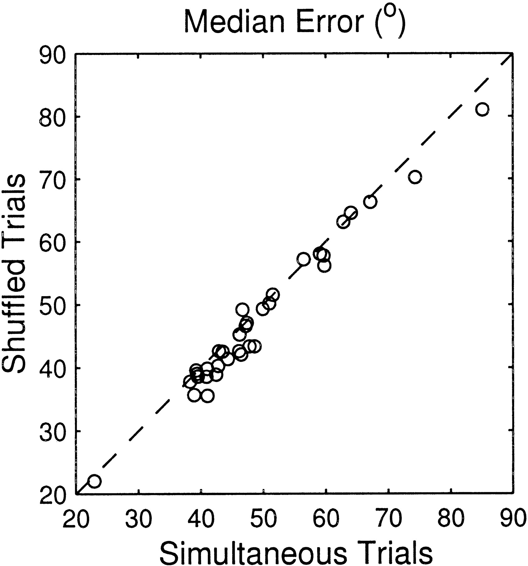
Comparison of the median errors of the network estimates for the ensemble spike patterns based on simultaneous trials and on random trials for each unit.
Comparison with psychophysical data
We compared the neural coding of sound-source locations, as represented by our ANN analysis, with the cat's performance in a localization task. May and Huang (1996) measured the accuracy of the cat's voluntary head orientation responses to broadband noise bursts presented from speakers in the frontal sound field. Source locations in that study were restricted within ±90° in azimuth. We trained and tested an ANN with input vectors consisting of spike patterns of the 128 units with the smallest median errors (as defined for the best-N-units configuration in the preceding section). We simulated the effects of a cat possibly basing its judgment on neurons from both sides of the cortical hemispheres by treating the responses for the even-numbered units as if they had been recorded from the contralateral (left) hemisphere. This was done by reversing the sign of the target azimuths for those units. To mimic the cat's task in the experiment by May and Huang (1996), we used neural responses to azimuths between −80° and +80° only, and we disregarded ANN estimates to other than frontal locations. The other conditions of the ANN analysis were the same as the best-N-units (nonsimultaneous) ensemble conditions.
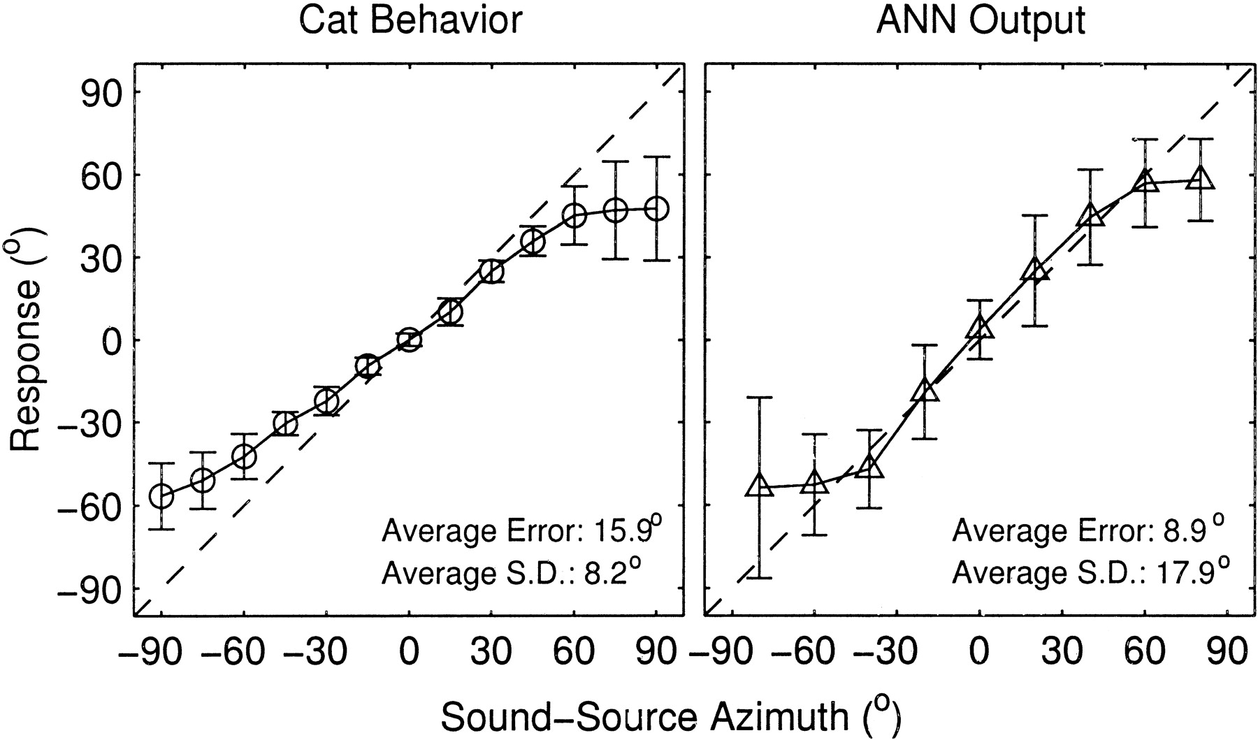
Figure 13 summarizes the responses of behaving cats (left) and the ANN (right). Means and SDs of orientation responses of psychophysical listeners are indicated by circles and error bars, respectively, for each target speaker azimuth [May and Huang (1996), average data from their Table 1]. Triangles and error bars show the means and SDs, respectively, for ANN estimates based on ensemble spike patterns for one trial. The cat behavior tended to show a systematic undershoot in responses; that is, responses were biased toward frontal locations. In contrast, the means of the neural data showed little undershoot except for the most lateral targets. The differences in the characteristics of undershoots probably did not perfectly reflect real sensory sensitivities to sound-source locations for either the ANN or the behaving cat. The undershoot in the psychophysical data was probably attributable primarily to head movements that fell short of the target speakers, particularly at the extreme lateral locations. For the neural data, the undershoot for lateral targets probably was caused by a bias to avoid rear locations that arose from ANN training that was restricted to frontal speakers only.

Responses of behaving cats and the ANN to sounds in frontal locations. Left, Circles and error bars indicate the means and SDs of the cats' head orientation responses to sound in the free field [from May and Huang (1996), their Table 1]. Right, Triangles and error bars show the means and SDs of network estimates based on a single presentation of a ensemble spike pattern consisting of 128 best units. The network was trained and tested for the frontal speakers (−80° to +80°), and network estimates to rear locations were disregarded. The final computation of SDs in the rightpanel omitted outlying points that were defined as points that were >3.0 SDs from the means in the initial computation of the SD.
Response variance was generally larger for the neural data than for the psychophysical data. Averages of the SDs across the speaker locations tested were 17.9° for the neural data (across 9 target locations) and 8.2° for the psychophysical data (across 13 locations). That difference also was reflected in the averages of unsigned errors across all locations, which were 8.9° for the neural data and 15.9° for the psychophysical data. SDs for the cat behavior tended to increase with increasing distance of the target from the midline, whereas the SD of the ANN performance was fairly constant across target locations except for the most lateral target locations. The small SDs of the cat's responses for target speakers around 0° could have reflected an artificial factor. In the psychophysical task, the cat was asked to fixate its head toward 0° in azimuth and elevation before a stimulus was presented followed by head orientation. Therefore, the response to a target at 0° required no head movement to achieve a correct response.
DISCUSSION
The results demonstrate (1) that spike patterns of unit ensembles recorded in response to single-sound presentations can signal the locations of sound sources, (2) that the relative counts and relative timing of spikes within ensemble spike patterns carry information about stimulus location, and (3) that the accuracy of localization by neural ensembles of adequate size approaches the accuracy of localization by cats in behavioral trials. Here, we comment on the strengths and weaknesses of the use of ANNs for analysis of neural coding, we consider features of ensemble spike patterns that do or do not appear to carry information related to sound-source location, and we compare sound localization by behaving animals with that by unit ensembles.
Use of artificial neural networks for analysis of stimulus coding
One might argue that the results of the present study could be obscured by our particular choice of network architecture and/or the way of representing spike patterns. Although we decided on the network and spike pattern configurations on the basis of preliminary analysis, our ANN configuration might have not been optimal to represent real coding efficiency by a neural ensemble. For that reason, our results represent a conservative estimate of information carried by the spike patterns. Another disadvantage of an ANN is that it tends to conceal the specific features that it uses to recognize spike patterns. For identifying specific information-bearing features, it is necessary to use alternative pattern recognition algorithms or to study carefully the connection weights and biases of trained ANNs. Nonetheless, we were able to infer information-bearing features in ensemble spike patterns empirically, for example, by removing information about absolute spike counts or about external reference time.
In sum, despite some disadvantages, the ANN method used in the present study has provided useful information for exploring complex ensemble coding by cortical neurons. An ANN can recognize high-dimensional input patterns without need for a priori specification of particular information-bearing features of the patterns. Also, it can solve nonlinear problems by incorporating nonlinear transfer functions. ANNs have been used successfully in several studies for recognition of single-unit and ensemble response patterns [auditory cortex (Middlebrooks et al., 1994, 1998; Xu et al., 1998, 1999a,b); visual cortex (Kjaer et al., 1994); retinal ganglion cells (Warland et al., 1997); somatosensory cortex (Nicolelis et al., 1998)].
Information-bearing features of unit ensemble spike patterns
An ANN was able to estimate stimulus locations with considerable accuracy on the basis of spike counts of unit ensembles. A comparison between the mean-spike-count and the relative-spike-count configurations (Fig. 9) revealed that the relative spike count among units could account for most information carried by the ensemble spike counts and that the absolute strength of unit activity is not important for location coding. Coding of sound-source locations by absolute spike counts is confounded to some degree by the sensitivity of spike counts to the stimulus SPL. Relative counts among units are somewhat less sensitive to the stimulus SPL (Furukawa et al., 1999). One can see a form of a relative-count code in the “population vector” hypothesis (Georgopoulos et al., 1986). Neurons in the primate motor cortex are broadly tuned to certain directions (“preferred directions”) of arm movement. The population vector hypothesis has proposed that the direction of arm movement could be predicted by a vector sum of the preferred directions of a population of cortical neurons, weighted by the spike counts of the neurons. In that model, the estimated arm directions are determined by the relative spike count of the neurons, and absolute spike counts are not directly relevant. It was not feasible to apply the population vector method directly to the auditory cortical neurons, however, because the spike-count tuning for sound-source location was generally too irregular to be modeled with a simple function as was used in the motor cortex work. Instead, we could determine the weights on spike counts empirically by training an ANN.
A comparison of the full-pattern and the count-only configurations demonstrated that the spike timing of unit ensembles could provide location-related information additional to ensemble spike counts. A similar result was observed by Nicolelis et al. (1998) using an ANN algorithm for identifying skin stimulation locations on the basis of ensemble spike patterns. In that study, the ANN performance was degraded somewhat when spike patterns were expressed in successively coarser resolution, but a reasonable level of accuracy was maintained even when the ANN inputs were spike counts only. Note, however, that the effect of bin width was observed only in cortical area SII and not in other areas tested. This may indicate that the relative importance of spike timing information varies across cortical areas.
An ANN was able to estimate accurately stimulus locations on the basis of the relative spike timing across units without an external reference to the time of stimulus onset. This result is consistent with studies that have shown stimulus azimuth sensitivities of relative spike timing between pairs of cortical neurons (Eggermont, 1998; Furukawa et al., 1998; Middlebrooks, 1998). We failed, however, to demonstrate that the pattern of spike timing within spike patterns of single units (i.e., interspike intervals) could carry sound-location information. This was rather surprising because raster plots or poststimulus-time histograms of single units often show the dispersion of spike timing somewhat varying with stimulus location (see Figs. 3, 4). Probably, interspike intervals are not a reliable code because cortical neurons generally have low spike probabilities, often averaging ∼1 spike per trial.
Comparison of the ANN performance between simultaneous- and shuffled-trial conditions pertains to the stimulus coding by coherent spiking activities across units that has been observed in simultaneous recording from multiple neurons (Abeles and Gerstein, 1988; Vaadia et al., 1995; deCharms and Merzenich, 1996; Hatsopoulos et al., 1998;Maynard et al., 1999) and to the correlation across neurons in the trial-by-trial variability of neural responses to the same stimulus (neural noise) (Eggermont, 1992; Gawne and Richmond, 1993;Zohary et al., 1994; Shadlen et al., 1996; Lee et al., 1998a,b; Oram et al., 1998). Our analysis showed little effect of trial shuffling (Fig.12), which was also found by Nicolelis et al. (1998) who studied tactile stimulus coding in the primate somatosensory cortex using ANN algorithms. As for coherent spiking activities, between-neuronal correlation was probably dominated by synchrony to the stimulus, and little additional correlation could be revealed by our methods. In terms of the effect of neural noise correlation, possible interpretations include that (1) there was no significant level of noise correlation, (2) major information-bearing features in ensemble spike patterns were insensitive to the correlation of noise, and/or (3) the trained ANNs for the simultaneous- and shuffled-trials conditions used somewhat different decoding strategies. Clearly, it is premature to draw strong conclusions from the present analysis. It is possible that our experimental and analysis methods simply did not have enough sensitivity to detect subtle effects of trial-by-trial coherent spiking activities or noise correlation between units. Anesthesia likely has some impact on mechanisms associated with neural synchrony. Multiunit spikes as found in most of our recordings could have obscured information represented by precise spike timing. Also, the effect of noise correlation should be studied by incorporating explicit specification of neural signal and noise, which was beyond the scope of the present study.
Sound localization by unit ensembles compared with animal behavior
Our previous studies have shown that neural signaling of sound-source location by single units in cortical area A2 correlates well with human sound localization judgments under conditions in which human listeners show accurate or systematically inaccurate localization (Xu et al., 1999a,b). Thus, we expected that ensemble spike patterns based on an appropriate number and selection of cortical units would show comparable coding accuracy with that of behaving animals. The ANN performance monotonically improved with increasing size of the neural ensemble, and the median error for the 128 best units was as small as 15.3° (Fig. 11).
Localization performance by an ANN based on the spike patterns of 128 units differed in detail from localization by behaving cats (May and Huang, 1996), particularly in the characteristics of the undershoot and in the magnitude of the variance (Fig. 13). Considering the differences between the studies in experimental procedure and in the animal's state (e.g., anesthetized vs awake), we regard the differences in mean error and variance between the ANN responses and psychophysical data as relatively small. Thus, it is possible that under more appropriate and comparable conditions, the localization performance of a behaving cat could be accounted for by the activities of an ensemble comprising a modest number of cortical neurons.
Concluding remarks
Overall, the present study demonstrated the effectiveness of neuronal ensemble codes in sound-source localization. As suggested by the significance of relative spike count and relative spike timing, coding by ensembles of neurons probably involves more than simple sums of information carried by individual units. Further studies will be necessary to identify details of information-bearing features and the neural mechanisms that can decode the features. Nonetheless, similarities in localization performance between spike patterns of neuronal ensembles and behaving animals should encourage further research on cortical roles and mechanisms for auditory space perception.
Footnotes
This work was supported by National Institutes of Health Grants PO1-DC00078 and T32-DC00011. Multichannel recording probes were graciously provided by the University of Michigan Center for Neural Communication Technology, which is supported by National Institutes of Health Grant P41-RR09754. We thank Zekiye Onsan for technical assistance. David Anderson, Brian Mickey, and Ewan Macpherson provided constructive comments on previous versions of this manuscript.
Correspondence should be addressed to Dr. John C. Middlebrooks, Kresge Hearing Research Institute, University of Michigan, 1301 East Ann Street, Ann Arbor, MI 48109-0506. E-mail: jmidd{at}umich.edu.


