QUICK SEARCH:   [advanced] Author: Keyword(s): Year:  Vol:  Page:

HOME  |   SEARCH  |   ARCHIVE  |   SUBSCRIBE  |   CONTACT  |   HELP

This Article Abstract Full Text (PDF) Submit an eLetter Alert me when this article is cited Alert me when eLetters are posted Alert me if a correction is posted Citation Map Services Email this article to a friend Similar articles in this journal Similar articles in Web of Science Similar articles in PubMed Alert me to new issues of the journal Download to citation manager Citing Articles Citing Articles via HighWire Citing Articles via Web of Science (110) Citing Articles via Google Scholar Google Scholar Articles by Alonso, J.-M. Articles by Reid, R. C. Search for Related Content PubMed PubMed Citation Articles by Alonso, J.-M. Articles by Reid, R. C.

 Previous Article  |  Next Article 

The Journal of Neuroscience, June 1, 2001, 21(11):4002-4015

Rules of Connectivity between Geniculate Cells and Simple Cells in Cat Primary Visual Cortex

Jose-Manuel Alonso^{1, 2}, W. Martin Usrey^{1, 3}, and R. Clay Reid^{1, 4}

¹ Laboratory of Neurobiology, The Rockefeller University, New York, New York 10021, ² Department of Psychology, University of Connecticut, Storrs, Connecticut 06269, ³ Center for Neuroscience, University of California, Davis, Davis, California 95616, and ⁴ Department of Neurobiology, Harvard Medical School, Boston, Massachusetts 02115

	ABSTRACT

TOP ABSTRACT INTRODUCTION MATERIALS AND METHODS RESULTS DISCUSSION REFERENCES

Hundreds of thalamic axons ramify within a column of cat visual cortex; yet each layer 4 neuron receives input from only a fraction of them. We have examined the specificity of these connections by recording simultaneously from layer 4 simple cells and cells in the lateral geniculate nucleus with spatially overlapping receptive fields (n = 221 cell pairs). Because of the precise retinotopic organization of visual cortex, the geniculate axons and simple-cell dendrites of these cell pairs should have overlapped within layer 4. Nevertheless, monosynaptic connections were identified in only 33% of all cases, as estimated by cross-correlation analysis. The visual responses of monosynaptically connected geniculate cells and simple cells were closely related. The probability of connection was greatest when a geniculate center overlapped a strong simple-cell subregion of the same sign (ON or OFF) near the center of the subregion. This probability was further increased when the time courses of the visual responses were similar. In addition, the connections were strongest when the simple-cell subregion and the geniculate center were matched in position, sign, and size. The rules of connectivity between geniculate afferents and simple cells resemble those found for retinal afferents to geniculate cells. The connections along the retinogeniculocortical pathway, therefore, show a precision that goes beyond simple retinotopy to include many other response properties, such as receptive-field sign, timing, subregion strength, and size. This specificity in wiring emphasizes the need for developmental mechanisms (presumably correlation-based) that can select among afferents that differ only slightly in their response properties.

Key words: visual cortex; simple cell; thalamus; thalamocortical; LGN; correlated firing

	INTRODUCTION

TOP ABSTRACT INTRODUCTION MATERIALS AND METHODS RESULTS DISCUSSION REFERENCES

Although separated by a single synapse, geniculate cells and cortical simple cells have very different response properties. Geniculate cells have receptive fields with a circular center and a concentric, antagonistic surround. Simple cells have receptive fields with elongated, parallel subregions. According to the original hypothesis of Hubel and Wiesel (1962), simple receptive fields are constructed from the convergence of geniculate inputs with receptive fields aligned in visual space. This hypothesis has received experimental support for simple cells in layer 4 of cat visual cortex (Reid and Alonso, 1995, 1996; Ferster et al., 1996; Chung and Ferster, 1998). Specifically, if the receptive-field center of a geniculate cell overlaps a simple-cell subregion of the same sign (ON or OFF), then there is a high probability that the simple cell and the geniculate cell will be connected. Otherwise, the probability of finding a connection is almost zero (Reid and Alonso, 1995).

The position and sign of receptive fields, however, may not be the only relevant factors in determining connectivity. Differences in response timing (Cleland et al., 1971a; Hoffmann et al., 1972; Mastronarde, 1987a,b; Humphrey and Weller, 1988; Wolfe and Palmer, 1998), receptive-field size [for instance X vs Y cells (Enroth-Cugell and Robson, 1966; Hochstein and Shapley, 1976)], or asymmetries in the shape of geniculate receptive fields (Daniels et al., 1977; Vidyasagar and Urbas, 1982; Schall et al., 1986; Soodak et al., 1987) could also play a role.

The development of precise connections between the lateral geniculate nucleus (LGN) and the visual cortex is likely based on correlations between presynaptic and postsynaptic activity (Stent, 1973; Changeux and Danchin, 1976; Stryker and Strickland, 1984; Miller et al., 1989; Goodman and Shatz, 1993; Weliky and Katz, 1997). Consequently, receptive-field parameters such as size and response timing should be important in determining wiring specificity. To test this hypothesis, we examined the receptive-field properties of pairs of geniculate and cortical neurons that were monosynaptically connected as estimated by cross-correlation analysis. Our results show that at least four receptive-field properties tend to be matched in connected pairs: sign, position, timing, and size. Moreover, the strength of a geniculocortical connection, the efficacy or contribution, is related to the degree of the receptive-field match.

	MATERIALS AND METHODS

TOP ABSTRACT INTRODUCTION MATERIALS AND METHODS RESULTS DISCUSSION REFERENCES

Surgery and preparation

Cats weighing 2.5-3 kg were initially anesthetized with ketamine (10 mg/kg, i.m.) and then with thiopental sodium (20 mg/kg, i.v., supplemented as needed). Lidocaine was injected subcutaneously or applied topically at all points of pressure or possible sources of pain. A tracheotomy was performed, and the animal was placed in the stereotaxic apparatus. Temperature (37.5-38°C), an electrocardiogram, EEG, and expired CO₂ (27-33 mmHg) were monitored throughout the experiment. The level of anesthesia was maintained by a continuous infusion of thiopental sodium (2-3 mg · kg¹ · hr¹, i.v.). If physiological monitoring indicated a low level of anesthesia, additional intravenous thiopental was given, and the rate of the continuous infusion was increased. Two holes were made in the skull, centered in the stereotaxic coordinates posterior 3 mm, lateral 2 mm for the striate cortex and anterior 6 mm, lateral 8 mm for the LGN. The dura mater was removed, and the two craniotomies were filled with agar to minimize brain movements. Animals were paralyzed (Norcuron, 0.2 mg · kg¹ · hr¹, i.v.) and respired through an endotracheal tube. To minimize respiratory movements, the animal was sometimes suspended from a lumbar vertebra, and a pneumothorax was performed. Posts attached to the stereotaxic frame were glued to the eyes to minimize movements. Pupils were dilated with 1% atropine sulfate, and the nictitating membranes were retracted with 10% phenylephrine. The positions of the area centralis and the optic disk were plotted with the aid of a fundus camera.

Electrophysiological recordings and data acquisition

Simultaneous cortical and geniculate recordings were made with two single electrodes in initial experiments. In later experiments, a matrix with seven independently moveable electrodes was used for the recordings in the lateral geniculate nucleus (Eckhorn and Thomas, 1993). Most cortical recordings were made near the occipital pole, near the representation of area centralis, where the area 17/18 border is several millimeters from the midline (Tusa et al., 1978). Most simple cells were recorded in layer 4. Although we did histology in some experiments, cortical layer 4 was identified in most cases by electrode depth, the strong hash produced by the geniculate afferents, and the presence of simple cells. In all cases in which histology was performed, the location of electrolytic lesions confirmed that recordings were made in layer 4. We cannot reject the possibility that some simple cells may have been recorded in nearby layers, particularly layer 3. Because we were careful not to record deep in the cortex (virtually all penetrations were normal to the cortical surface), it is unlikely we recorded cells in layer 6.

Recorded signals were amplified, filtered, and collected by a computer running the Discovery software package (Datawave Systems, Longmont, CO). Provisional identification of spike waveforms was done during the experiment and then revised in off-line analysis. The quality of spike isolation was based on cluster analysis software, the presence of a refractory period in the autocorrelogram, and in some cases reviewing stored analog data.

Analysis of cross-correlations

Cross-correlations were calculated from spike trains obtained during stimulation with sine-wave gratings and/or white noise. The raw cross-correlations contain features influenced both by the stimulus and by connections between neurons. Peaks caused by monosynaptic connections are easy to detect because they have a rise time of ~1 msec and a delay between geniculate and cortical firing of 2-4 msec (Tanaka, 1983; Reid and Alonso, 1995; Alonso et al., 1996; Alonso and Martinez, 1998; Usrey and Reid, 1999; Usrey et al., 2000). To judge the significance of monosynaptic peaks, we used a procedure that worked for data obtained with grating stimuli as well as white noise. The correlation was first bandpass filtered between 75 and 700 Hz to capture only the fastest correlations (Reid and Alonso, 1995). These frequencies are faster than most visual responses, so this procedure removes stimulus-dependent correlations just as effectively as does shuffle subtraction. If the filtered correlation between 0.5 and 4.5 msec was 2.8 SD above the baseline noise (corresponding to 0.2% probability per bin, assuming a normal distribution), this was considered a positive correlation (Reid and Alonso, 1995). In addition, only positive correlations with peak magnitudes 6% greater than the baseline were considered significant. To avoid false negatives because of insufficient data, any correlogram with <50 spikes in the baseline was rejected from our final sample (Reid and Alonso, 1995).

For the correlations that were judged significant by the above criteria, an independent procedure was used to calculate the strength of the correlation. The "peak magnitude" was calculated by integrating the raw (unfiltered) correlogram between 0.5 and 4.5 msec and then subtracting the baseline. The "baseline" was defined as the integral of the correlogram over 2 msec intervals immediately before and after the peak. The peak magnitude can be normalized in two different ways to yield distinct measures of the strength of a connection: "efficacy" and "contribution" (Levick et al., 1972). The efficacy is the percentage of geniculate spikes that were followed by a cortical spike within a time window of 0.5-4.5 msec: efficacy = (peak magnitude)/(total number of geniculate spikes). The contribution is the percentage of cortical spikes that were preceded by a geniculate spike within a time window of 0.5-4.5 msec: contribution = (peak magnitude)/(total number of cortical spikes). Because different normalizations are possible, all correlograms are shown in terms of raw spike counts, but the total number of presynaptic and postsynaptic spikes is given in the figure legends.

Visual stimulation and receptive-field mapping

An AT-Vista graphics card (Truevision, Indianapolis, IN) was used to generate visual stimuli. The frame rate of the monitor was usually set to 128 Hz (80 and 100 Hz for the initial experiments). The receptive fields of each cortical unit were mapped both by hand and by use of binary white-noise stimuli [generated with an m-sequence (Reid and Shapley, 1992; Sutter, 1992; Reid et al., 1997)]. Spatially, the white-noise stimulus consisted of a 16-by-16 grid of square regions (pixels). The pixels were small enough to map receptive fields with a reasonable level of detail (0.2-0.4° for eccentricities of <10°, which usually corresponded to two to three pixels across for an LGN center or a cortical subregion). Unlike with sparse noise (Jones and Palmer, 1987), white noise allowed us to map weak flanks in simple cells when using small (0.4°) pixels, modulated at a high rate (once every two frames, or 40-64 Hz).

Receptive-field maps were calculated by reverse correlation. For each delay between stimulus onset and neural impulse firing, the average spatial stimulus was calculated. The resulting function, the "spatiotemporal receptive field" (or, more properly, the spatiotemporal weighting function), RF(x,y,t), depends on the spatial variables x and y (which range from 1 to 16, in units of pixels) and time t, binned at the same rate that the stimulus was changed. As outlined elsewhere (Reid et al., 1997), we normalized the receptive-field maps (or, more formally, the first-order spatiotemporal kernels) in units of spikes per second. For a given pixel and a delay of N frames, a value of +1.0 means that the instantaneous rate of the neuron increased on average 1.0 spike/sec N stimulus frames after the pixel was white. A value of 1.0 means that the instantaneous rate of the neuron increased 1.0 spike/sec after the pixel was black. Although the method cannot distinguish ON excitation from OFF inhibition and vice versa, we use the term ON responses for positive values and OFF responses for negative values.

Analysis of receptive-field overlap

To compare spatial aspects of the receptive field, a "spatial receptive field" (or spatial weighting function) needed to be defined. This problem is not entirely trivial, because the spatial profile of both geniculate neurons and simple cells is different for different delays between stimulus and response (McLean and Palmer, 1989; Reid et al., 1997). We therefore defined the spatial receptive field by the following multistep algorithm. First, we defined the time of the first maximum, t_max1, in two stages. The response magnitude for each time bin was defined as the pixel with the strongest response at that bin summed with all contiguous pixels of the same sign. The first local maximum of this response magnitude was defined as t_max1. To avoid spurious initial peaks, a subsequent local maximum was used if it was >1.5 times larger than the first local maximum. Next, we defined the spatial receptive field as the average of the receptive fields at t_max1  1, t_max1, and t_max1 + 1. In a few cases, the response changed sign (termed the "rebound," see below) in frame t_max1 + 1. In these cases, we only averaged the frames t_max1  1 and t_max1. Our averaged receptive fields had better signal to noise than did the spatial receptive fields obtained at a single time bin and also included features that were sometimes lost in the single frame, such as a slower surround or a slower simple-cell subregion.

Given the spatial receptive fields of LGN cells and simple cells, we used two approaches to quantify overlap. In the first approach, we modeled the geniculate receptive field as two-dimensional Gaussians (Rodieck, 1965) and simple cells as Gabor functions (Marcelja, 1980) and then compared various parameters of the two functions. In the second approach, we calculated two forms of a normalized dot product of the two receptive fields, each of which yields a single number that ranges between 1.0 and +1.0 (see Usrey et al., 1999).

Gaussian and Gabor function fits. Geniculate cell centers were fit to two-dimensional Gaussian functions (with four parameters):
where A is the amplitude, x₀ and y₀ are the coordinates of the center of the receptive field, and  is the SD, or space constant, of the Gaussian. Note that elsewhere (Reid and Alonso, 1995; Alonso et al., 1996) we used a different convention: 2² in the denominator rather than ². Simple cells were fit to Gabor functions, the product of an elliptical Gaussian and a sinusoidal term:
The variables u, v, and w are the spatial axes rotated by _Gau or _cos: u = cos(_Gau)x + sin(_Gau)y, v = sin(_Gau)x + cos(_Gau)y, and w = cos(_cos)x + sin(_cos)y. _u and _v are the space constants of the major and minor axes of the Gaussian, and f and  are the spatial frequency and the phase of the sinusoidal component.

A number of parameters were calculated from the Gaussian and Gabor function fits. First, the "radius" of the Gaussian was defined as the diameter of the circle defined by 20% of the peak value. Similarly, the "width" and "length" of a subregion in the Gabor function were obtained from the curve defined by 20% of the peak value. The "aspect ratio" of a subregion was defined as the ratio of this length to width. Finally, the "sign" of the overlap (same or opposite) was determined by the value of the simple-cell Gabor function at the center of the geniculate Gaussian.

Unlike these other spatial parameters, the "strength" of a cortical subregion was obtained directly from the data. For this purpose, up to three subregions were defined from the spatial receptive field (see above) by taking all of the same-sign contiguous pixels starting with a local maximum. To avoid spuriously large subregions, only data larger than twice the SD of the baseline noise were included in this procedure. The baseline noise was taken as the receptive-field values for very long delays (greater than ~150 msec). The strength of a subregion was obtained by summing the response values over all points in its contiguous region. The strength was used to rank order the subregions from strongest to weakest (see Fig. 12). This ordering was used, rather than the Gabor fit, to ensure that the relative strengths of flanks were well represented by the actual data.

Normalized dot product. The overlap was also quantified as a scalar by taking the dot product of two spatial receptive fields:

The raw dot product is difficult to interpret, so we normalized it in two ways. In the first normalization [termed "overlap" (Usrey et al., 1999)], the raw dot product is divided by ((RF₁·RF₁) (RF₂·RF₂))^1/2 to yield a measure of correlation. Overlap is equal to +1.0 if the two receptive fields are identical to within a positive scale factor and perfectly superimposed; it is equal to 1.0 if they are equal but of opposite sign. Because simple receptive fields and geniculate receptive fields have very different spatial configurations, the overlap should never be 1.0. A second normalization is achieved by shifting the relative position of the two receptive fields to find the dot product with the largest possible absolute value. The original dot product normalized by this largest possible dot product is called "relative overlap." The relative overlap can also range between +1.0 (best overlap, same sign) and 1.0 (best overlap, opposite sign). By definition, any two receptive fields, even if they are mismatched in size or shape, can have a relative overlap of 1.0 or 1.0 if they are appropriately placed. In summary, overlap is a measure of relative position and similarity (for instance, of receptive-field size); relative overlap is a measure of relative position alone.

Analysis of the time course of visual responses

The "impulse response" (or temporal weighting function) at a single spatial location in the receptive field was defined simply by the evolution of the receptive field as a function of t. Impulse responses of the center of the geniculate receptive field or of a cortical subregion were obtained by summing over the same-sign contiguous pixels in the spatial receptive field (defined above). The impulse responses of cortical subregions are somewhat hard to define, however, because in many cases the impulse responses of different pixels in a subregion have different time courses (Movshon et al., 1978), particularly for directionally selective cells (Reid et al., 1987, 1991; McLean and Palmer, 1989; DeAngelis et al., 1993a,b). Therefore, to compare the time courses of a geniculate center and the overlapped cortical subregion (see Figs. 8, 9), only the intersection of the geniculate center and the cortical subregion was considered. When the geniculate cell was overlapped with two cortical subregions, the subregion of the sign that overlapped the strongest pixel in the geniculate receptive field was used.

Most impulse responses of geniculate cells and simple cells are biphasic. For example, for an ON-center geniculate cell, there is first a positive ON response (first phase) and then a negative OFF rebound (second phase). The timing and relative amplitude of onset and rebound vary considerably among geniculate cells. We calculated three different temporal parameters from the impulse responses of the overlapped geniculate center and simple-cell subregions: the peak time of the first phase, the zero crossing (see Fig. 7A,B below), and the rebound time. These parameters were interpolated, using a cubic spline, from impulse responses calculated at the stimulus-update rate (see Usrey et al., 1999). By our convention, the 0.0 msec bin corresponds to responses occurring in the first stimulus frame (for instance between 0.0 and 20.0 msec at 50 Hz). Before performing the spline interpolation, however, we assigned each point to the middle of the bin. Because most responses were biphasic, the identities of the peak time (the time when the first phase reached its maximum), the zero crossing, and the rebound time (maximum of the second phase) were usually unambiguous.

We also calculated a "rebound index," a parameter related to the shape of the response. The rebound index [termed transience elsewhere (Usrey and Reid, 2000)] was defined as the following: 1^.(rebound magnitude)/(peak magnitude). The peak magnitude is the integral of the response before the zero crossing; the rebound magnitude is the integral of the response after the zero crossing (see Fig. 7C below). The rebound index is similar to the "biphasic index" of Cai et al. (1997), which used the peaks of each phase rather than their integrals.

A small proportion of LGN cells had rebound indices greater than one; in other words the rebound was stronger than the initial peak. For instance, what we call an OFF cell could have an ON rebound stronger than the initial OFF peak. If such a cell summed its responses linearly, it would be expected that its response to a luminance step (as opposed to an impulse) would start with a small OFF response, followed by a more sustained ON response. This is true because a step response should be equal to the integral of the impulse response (Gielen et al., 1982; see Usrey and Reid, 2000). Other studies using white-noise techniques (Cai et al., 1997; Wolfe and Palmer, 1998) have found that, in most cases, such a cell would in fact prove to be an ON-center lagged cell (Mastronarde, 1987a,b) when tested with step stimuli. We nevertheless chose to call these cells OFF cells; in other words, the sign of the cell (or subregion) was defined by the initial phase of the impulse response.

There were 36 LGN cells for which the second phase was greater than the first phase [23 cells with a rebound index between 1 and 1.2 (mainly cells with large receptive fields; likely to be Y cells, see below), 8 cells between 1.2 and 1.5, and 5 cells >1.9]. Almost certainly, the cells with a rebound index >1.9 were lagged cells (Cai et al., 1997; Wolfe and Palmer, 1998). Many of the other cells with a rebound index >1.2 might have been classified as lagged cells if we had performed the appropriate tests (Mastronarde, 1987a; Saul and Humphrey, 1990; Lu et al., 1995). Because the sign (ON or OFF) of these cells is a matter of convention, depending on whether the first or second phase is used, we deal with them separately in Results (at the end of Time course of the response).

It should be noted that the half-rise time (the time it takes to reach half of the peak response) has been used to distinguish between lagged and nonlagged cells in most studies, starting with the first study of lagged cells (Mastronarde, 1987a). When cells are characterized by their impulse responses, however, the very long half-rise times are seen almost exclusively when a large second phase is considered the "peak." For instance, Cai et al. (1997) found a bimodal distribution of half-rise times but a continuum of response waveforms. The bimodal distribution of half-rise times was entirely caused by the sharp cutoff for considering the second phase the peak. Similarly, in our sample, the cells with large rebound indices would have had much longer half-rise times if we had arbitrarily assigned the second phase to the peak, for instance, when the rebound index was of a certain magnitude (perhaps 1.2 or 1.5).

Finally, because the direction selectivity of cortical simple cells is closely related to the relative timing of the responses in different parts of the receptive field (Reid et al., 1987, 1991; McLean and Palmer, 1989), we calculated a predicted direction index from each cortical spatiotemporal receptive-field map. Given a spatiotemporal receptive field, it is possible to predict the response to any spatiotemporal stimulus by convolving the receptive field with the stimulus. For the case of drifting sinusoidal gratings, this convolution can be calculated easily by taking the three-dimensional Fourier transform of the spatiotemporal receptive field (see Jones et al., 1987). The amplitude of each complex number in the Fourier transform corresponds to the expected amplitude of the response to a drifting grating of a given spatial frequency, angle, and temporal frequency. For each spatiotemporal receptive field, we found the angle and spatial frequency of the grating that would evoke the strongest response for 4 Hz drift. The choice of temporal frequency was arbitrary but was chosen because it typically evokes strong responses in simple cells and has been used in past studies of directionality in simple cells (Reid et al., 1987, 1991). The predicted directional index (DI) was defined as the difference between the predicted responses to this grating and the predicted response to an identical grating moving in the opposite direction, divided by the sum of the two responses. The predicted directional index calculated from static stimuli is typically approximately one-third of the value of the actual directional index measured with drifting gratings (Reid et al., 1987, 1991). We defined neurons with a predicted directional index of >0.3 as directionally selective.

	RESULTS

TOP ABSTRACT INTRODUCTION MATERIALS AND METHODS RESULTS DISCUSSION REFERENCES

We recorded from 221 pairs of geniculate cells and simple cells with spatially overlapping receptive fields. Both geniculate and cortical receptive fields were simultaneously mapped with white-noise stimuli by reverse correlation. Geniculocortical monosynaptic connections were identified by cross-correlation analysis (Perkel et al., 1967; Tanaka, 1983; Reid and Alonso, 1995; Usrey et al., 2000). Of the 221 pairs, 180 had sufficient spikes in the baseline of the correlograms to be included in our analysis (Reid and Alonso, 1995) (see Materials and Methods); 61 of these pairs had statistically significant positive correlations. Correlograms consistent with monosynaptic connections were most frequently found between cells whose responses were similar with respect to the following attributes.

(1) Receptive-field sign (ON or OFF): the geniculate center overlapped a simple-cell subregion of the same sign.

(2) Receptive-field position: the peak-to-peak distance between the geniculate center and the simple-cell subregion (in units of subregion width) was less than one along the length of the subregion and less than one-half along the subregion width.

(3) Time course of the response: the geniculate center and the simple-cell subregion evoked visual responses with similar time courses.

(4) Subregion strength: the geniculate center overlapped the strongest subregion of the simple cell.

(5) Receptive-field size: the diameter of the geniculate center was equal to or slightly larger than the width of the simple-cell subregion.

These five rules of connectivity are listed in order of strictness. Cell pairs that did not follow the first two rules were rarely connected. The last rule, however, gave only a slight increase in the probability of finding a monosynaptic connection. The results are organized with respect to these five rules of connectivity.

Receptive-field sign

In agreement with a previous study (Reid and Alonso, 1995), the probability of finding a monosynaptic connection between a geniculate cell and a simple cell depended strongly on the sign (ON or OFF) of the overlapping regions of the receptive fields. Monosynaptic connections were usually found when the geniculate center overlapped a simple-cell subregion of the same sign (e.g., ON superimposed with ON) and were rare when the receptive fields were of different sign (e.g., ON superimposed with OFF).

Monosynaptic connections were identified by cross-correlation analysis as positive peaks displaced from zero with short latencies and fast rise times (Fig. 1) (Perkel et al., 1967; Tanaka, 1983; Reid and Alonso, 1995; Swadlow, 1995; Alonso et al., 1996; Swadlow and Lukatela, 1996; Alonso and Martinez, 1998; Usrey et al., 2000). Each bin in the correlogram corresponds to the number of cortical spikes that occurred either before (negative times) or after (positive times) a geniculate spike. Statistically significant "monosynaptic peaks" (see Materials and Methods) could be obtained either by using a visual stimulus (white noise or drifting gratings) or in the absence of visual stimulation (for simple cells that had sufficient spontaneous activity). When using a visual stimulus, the fast positive peak was superimposed on a much slower stimulus-dependent correlation (Fig. 1, bottom left). In the absence of a visual stimulus only the positive peak was observed (Fig. 1, bottom right). We display most correlograms over a time window of ±50 msec to illustrate the difference between fast and slow correlations, which are caused by different mechanisms. Fast correlations are almost certainly the result of monosynaptic connections (Perkel et al., 1967; Tanaka, 1983; Reid and Alonso, 1995; Swadlow, 1995; Alonso et al., 1996; Swadlow and Lukatela, 1996; Alonso and Martinez, 1998; Usrey and Reid, 1999). Slow correlations, instead, are caused by the simultaneous stimulation of the geniculate and simple-cell receptive fields (Usrey and Reid, 1999).

View larger version (33K): [in this window] [in a new window]   Figure 1.   Monosynaptic connection between a geniculate cell and a simple cell with overlapping receptive fields of the same sign. Top, The receptive fields of the geniculate cell and the simple cell are shown as contour plots (gray lines, ON response; black lines, OFF response). The dotted cross marks the center of the geniculate receptive field. Both receptive fields were plotted at the same delays between stimulus and response (35-50 msec). The stimulus was updated every 15.5 msec. Bottom, Cross-correlograms show a fast positive peak displaced from zero, indicating a monosynaptic connection. When a drifting grating is used as a visual stimulus (left), the positive peak is superimposed on a slow stimulus-dependent correlation. In the absence of visual stimulation (right), the positive peak is seen superimposed on a flat baseline. The asterisk indicates that the positive peak was statistically significant (see Materials and Methods). Number of geniculate spikes: 10,310 (visual stimulus, drifting grating) and 9728 (no visual stimulus); number of simple-cell spikes: 3777 (visual stimulus) and 3927 (no visual stimulus). Bin width, 0.5 msec.

A sign mismatch, an ON geniculate center overlapping an OFF simple-cell subregion, is illustrated in Figure 2. As expected (Reid and Alonso, 1995), cross-correlation analysis revealed a slow correlation without a superimposed fast peak, which indicates the absence of a monosynaptic connection (Fig. 2, right). Similar flat correlograms were found in most cases of a sign mismatch between the geniculate and simple receptive fields. However, a difficulty with the "sign rule" is raised when a geniculate cell with a large receptive field covers more than one simple-cell subregion. The receptive field of this geniculate cell can be perfectly centered on a subregion of the same sign and still overlap adjacent subregions of different sign. This is an important issue that could not be addressed in a previous study because of the small sample size; cells with large receptive fields were discarded in Reid and Alonso (1995). Here, with a much larger sample, we were able to divide our geniculate centers into two groups based on receptive-field size relative to the superimposed cortical subregion: small (less than two subregion widths) and large (more than two subregion widths). Most cells within our group of "large receptive fields" are likely to be Y cells (Stoelzel et al., 2000; Yeh et al., 2000). As shown in Figure 3, these cells with large fields were still more likely to connect to a simple cell if the very center of the receptive field overlapped a subregion of the same sign.

View larger version (18K): [in this window] [in a new window]   Figure 2.   Geniculate cell and simple cell with spatially overlapping receptive fields of different sign that are not connected. Left, Middle, Receptive fields are shown. Conventions are described in Figure 1. Both receptive fields were plotted at the same delays between stimulus and response (32-52 msec). The stimulus was updated every 20 msec. Right, Flat correlation indicates the absence of a direct excitatory connection. Number of geniculate spikes: 67,111; number of simple-cell spikes: 8544. Bin width, 0.5 msec.

View larger version (42K): [in this window] [in a new window]   Figure 3.   Distribution of cell pairs with respect to receptive-field sign. Left, Number of connected (positive cross-correlation) and nonconnected (flat cross-correlation) cell pairs for geniculate cells with small (A) and large (B) receptive fields. Small geniculate centers are smaller than two simple-cell subregion widths. Large geniculate centers are larger than two simple-cell subregion widths. Total number of cell pairs, 180. Total number of positive correlations, 61. The percentages within each group are shown at the top of each histogram bar. Right, The efficacy and contribution from each connection. The arrow indicates a compression of the y-axis. Below the arrow, each division is 2.5%. Above the arrow, the scale is contracted by a factor of six. Cont., Contribution (open circles); Eff., efficacy (filled diamonds); Flat Xcorr, flat cross-correlation (open bar); Pos Xcorr, positive cross-correlation (filled bar).

Regardless of receptive-field size, geniculocortical connections were strongest when the receptive-field centers were of the same sign as the overlapping simple subregion. First, these connections tended to have a greater efficacy; a larger percentage of geniculate spikes were followed by a cortical spike (Fig. 3, right, filled diamonds). Second, they had a higher contribution; a larger percentage of cortical spikes were preceded by a geniculate spike (Fig. 3, right, open circles). In fact, the few connected geniculate cells that did not follow the sign rule usually had receptive-field centers located near the border between two simple-cell subregions (data not shown).

Receptive-field position

Geniculocortical connections were most often encountered when the geniculate center not only matched the sign of the overlapped simple-cell subregion but was also centered at the subregion peak (the position within the subregion that evoked the strongest responses). If the geniculate center was displaced from this peak (particularly along the width axis), the probability of finding a monosynaptic connection decreased.

We quantified the distance from the geniculate center to the subregion peak in all cell pairs in which the geniculate center overlapped a simple-cell subregion of the same sign (n = 90; only small geniculate centers with a diameter less than two cortical subregion widths were examined). For this analysis, we express distance in terms of cortical subregion width at 20% of the peak response, derived from a parametric fit to the spatial receptive field (a Gabor function; see Materials and Methods). Across the width axis (Fig. 4A), the probability of finding a connection was very low (2 of 13) when the distance between the geniculate center and the subregion peak was greater than one-half the subregion width. These are, by definition, the LGN cells with receptive-field centers near the border between subregions. Along the length axis (Fig. 4B), however, connections were still found at distances twice as large. Similarly, both the efficacy and contribution of the connections became weaker as the distance between the receptive fields increased (Fig. 4A,B). This analysis suggests that the receptive fields of the geniculate inputs to a simple cell are aligned in visual space; the scatter along the length of the subregion was approximately twice the scatter along the width. It is important, however, to emphasize that all aligned geniculate centers are contained within the limits of the "classical receptive field" of the simple cell. This can be demonstrated by measuring distance in units of the subregion length (Fig. 4C), rather than the subregion width (Fig. 4B). In this case, most of the connected LGN cells we found were centered within one length unit.

View larger version (34K): [in this window] [in a new window]   Figure 4.   Distribution of cell pairs with respect to the distance between their receptive fields. Number of connected (positive cross-correlation) and nonconnected (flat cross-correlation) cell pairs as a function of the distance between the LGN center and the peak of the simple-cell subregion, in both width and length, is shown. A, B, Distances were measured in units of simple-cell subregion widths. C, Because simple cells had differing aspect ratios (length/width), the distance in length is also given in units of subregion length. Only cell pairs with receptive fields of the same sign (e.g., ON superimposed with ON) and with small geniculate centers (<2 subregion widths) were selected (n = 90). Efficacies and contributions are shown to the right, as described in Figure 3. D, Histogram of aspect ratios for all overlapped subregions (n = 221; mean, 2.5 ± 0.8; median, 2.3) is shown. In A-D, single numerical values under histogram bars indicate the upper limit in a range.

The differences between Figure 4, B and C, are determined by the aspect ratio (length/width) of the cortical subunit. In our total population of cells, aspect ratios ranged from 1.17 to 5.45 (mean, 2.5 ± 0.8; median, 2.3; Fig. 4D). These values are somewhat low in comparison with most studies of simple cells [range, 1.7-12; median, ~5 (Jones and Palmer, 1987); range, 2-12; median, ~3.5 (Gardner et al., 1999); range, 1-4; mean, 1.7 (Pei et al., 1994)] but are consistent with studies that concentrated on layer 4 simple cells [~2 (Bullier et al., 1982); mean, 2.3 ± 0.8 (Martinez et al., 1999)].

A second approach to quantifying receptive-field overlap is to define a single scalar that captures the degree to which the geniculate and simple receptive fields are well matched. A dot product between the two receptive fields, calculated by taking the product of the two receptive fields at each pixel and then summing, is one such measure. From the dot product, we derived two parameters, the overlap and the relative overlap, that differ only by the way they are normalized. As noted in Materials and Methods, both parameters can range between 1.0 and 1.0. The overlap of two receptive fields is equal to 1.0 (or 1.0) if they are spatially identical within a positive (or negative) scale factor and are perfectly overlapped. If the two receptive fields have different spatial configurations, the overlap can never be 1.0. The relative overlap is 1.0 if the two receptive fields are overlapped as best they can be, despite differences in spatial configuration (for instance if one is much bigger than the other, or if one is very elongated). Both measures, relative overlap (Fig. 5A) and overlap (Fig. 5B), are highly correlated with the probability of an LGN cell being connected to a potential cortical target.

View larger version (44K): [in this window] [in a new window]   Figure 5.   Distribution of connected cell pairs with respect to the normalized dot product of their receptive fields. Two forms of normalized dot products are shown (see Materials and Methods). A, The relative overlap. B, The overlap. The relative overlap is 1.0 if the two different receptive fields are in the optimal relative position. The overlap is 1.0 if the two receptive fields are identical. Data shown are only for pairs with same-sign overlapped subregions (n = 104). Efficacies and contributions are shown to the right (as described in Fig. 3); data points from large receptive fields (>2 subregion widths) are shown with large symbols.

Time course of the response

In addition to the sign and position of the receptive fields, other response properties also influenced the likelihood of finding a connection. Among these, timing was particularly important. The time courses of visual responses differ considerably among both geniculate cells and simple cells (although as a population, responses in geniculate cells tend to be faster than those in simple cells). It might be expected that the timing of the geniculate inputs should match the timing of the simple-cell targets. This prediction is consistent with developmental models based on correlated neural activity (Miller et al., 1989; Miller, 1994) and also some models of direction selectivity (Saul and Humphrey, 1992). The models of direction selectivity explicitly consider the distinction between lagged and nonlagged cells in the LGN (Mastronarde, 1987a,b). Because we recorded from few lagged cells (and did not classify them with standard tests, see Materials and Methods), our results concerning timing pertain mostly to nonlagged and partially lagged geniculate cells (but see below).

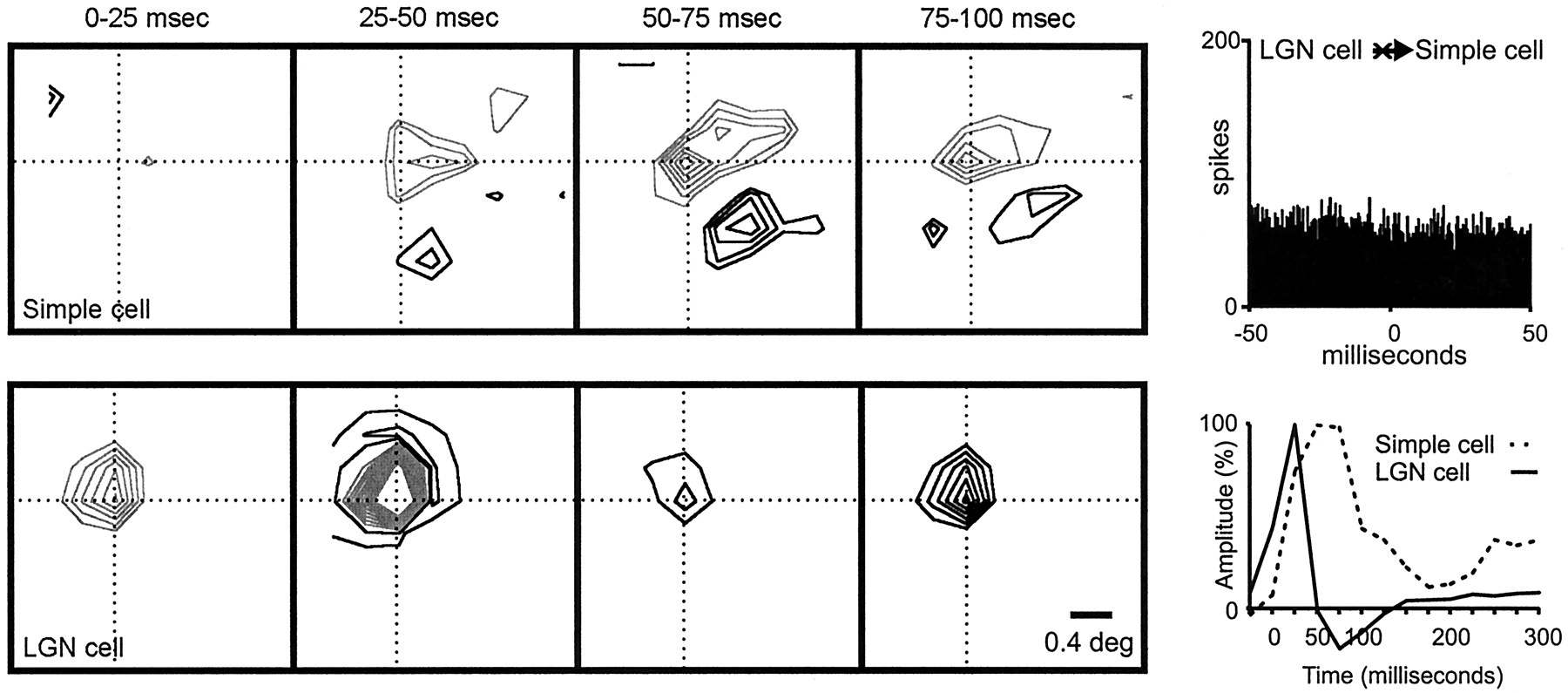
The white-noise method used in this study yields a detailed representation of both the spatial and temporal properties of a receptive field. Specifically, a series of receptive-field maps can be obtained for different times between the stimulus and response. Figure 6 shows an example of a receptive-field "movie" for two neighboring geniculate cells that were simultaneously recorded with a single electrode. The spatial receptive fields of these two cells were almost identical (same position, sign, and size), but their response time courses were very different. These timing differences are illustrated by the impulse responses calculated from the receptive-field series (Fig. 6, bottom). Each impulse response is obtained by plotting the summed responses from all pixels in the receptive-field center (see Materials and Methods) for each receptive-field frame (from Fig. 6, top). ON responses are represented as positive values, and OFF responses are represented as negative values. The response time courses of cell A and cell B differed in several ways. First, the impulse response for cell A was biphasic (the ON response was followed by an OFF rebound), whereas the impulse response for cell B was practically monophasic. Second, the response peaked 25 msec later (one stimulus frame) for cell B than for cell A. Third, the response lasted 75 msec longer for cell B (three stimulus frames). Cell A and cell B differed not only in the time course of their visual responses but also in the firing patterns. For example, the shortest observed interspike interval was longer for cell B than for cell A, as can be seen in the autocorrelograms (Fig. 6, bottom right). In summary, geniculate cell A and cell B differed in their temporal response properties (response latency, response duration, and rebound index) and in their interspike intervals but were spatially similar (receptive-field position, size, and response sign).

View larger version (38K): [in this window] [in a new window]   Figure 6.   Receptive fields and impulse responses from two neighboring geniculate cells. Spatially the receptive fields are very similar, but their timing is different. Top, A series of receptive-field frames calculated for each geniculate cell at different times after the stimulus is shown. Bottom, Left, The impulse responses (biphasic for cell A and monophasic for cell B) are shown. The labels on the x-axis show the lower limit of the time interval during which the stimulus was presented (e.g., 0 indicates 0-25). The stimulus was updated every 25 msec. Although not tested explicitly, the two cells most likely correspond to nonlagged (cell A) and partially lagged (cell B) cell types (Cai et al., 1997; Wolfe and Palmer, 1998). Right, Autocorrelograms are shown for each geniculate cell. The gap in the middle of the autocorrelogram is longer for cell B than for cell A, which indicates a longer refractory period. Number of spikes in the autocorrelogram of cell A: 21,698; number of spikes in the autocorrelogram of cell B: 4296.

The temporal parameters that differentiate cell A from cell B varied considerably among the entire population of geniculate cells and simple cells. We examined the distributions for some of these temporal parameters by calculating the impulse responses for both the simple cell and the geniculate cell. We examined only pixels within the intersection of the geniculate center and the simple-cell subregion. All parameters were interpolated from impulse responses calculated with a cubic spline. We calculated three different temporal parameters: peak time, zero-crossing time, and rebound time (see Materials and Methods and Fig. 7A,B). From these parameters, we also calculated several derived parameters that were useful in comparing response timing between LGN and cortex: peak time + zero-crossing time, duration from peak to zero-crossing time, and duration from peak to rebound. Finally, we calculated a parameter that characterized the shape of the impulse response: the rebound index or the ratio of the second phase of the impulse response over the first (see Materials and Methods and Fig. 7C). To make precise measurements, particularly of the rebound, we selected only impulse responses with good signal to noise (the maximum of the impulse response had to be >5 SD above baseline; n = 169). Data typically failed to meet this criterion when the simple-cell subregion was weak or was only partially overlapped by the geniculate center.

View larger version (27K): [in this window] [in a new window]   Figure 7.   Distribution of geniculate cells and simple cells with respect to the timing of their responses. The distribution of three parameters derived from impulse responses of geniculate and cortical neurons is shown. A, Peak time. B, Zero-crossing time. C, Rebound index. Peak time is the time with the strongest response in the first phase of the impulse response. Zero-crossing time is the time between the first and second phases. Rebound index is the area of the impulse response after the zero crossing divided by the area before the zero crossing. Only impulse responses with good signal to noise were included (>5 SD above baseline; n = 169).

Geniculate responses tended to peak faster and to be briefer than simple-cell responses. This can be appreciated from the distribution of peak times (Fig. 7A) and zero-crossing times (Fig. 7B) for the two populations. Similar distributions were seen for other parameters such as rebound time and total response duration (data not shown). In addition, geniculate cells and simple cells often differed in the relative strength of their rebounds or their rebound index (Fig. 7C; see Materials and Methods). Most simple cells had very weak rebounds. In contrast, geniculate cells displayed a range of rebound indices, some of them >1.0 (rebound stronger than the peak). Although the visual responses of simple cells and geniculate cells differed for all temporal parameters measured, there was considerable overlap between the distributions (Fig. 7). This overlap raises the following question: does connectivity depend on how well geniculate and cortical responses are matched with respect to time? For instance, do simple cells with fast subregions (early times to peak and early zero crossings) receive input mostly from geniculate cells with fast centers?

Figure 8 illustrates the visual responses from a geniculate cell and a simple cell that were monosynaptically connected. A strong positive peak was observed in the correlogram (shown with a 10 msec time window to emphasize its short latency and fast rise time). In this case, an ON central subregion was well overlapped with an ON geniculate center (precisely at the peak of the subregion). Moreover, the timings of the visual responses from the overlapped subregion and the geniculate center were very similar (same onset, ~0-25 msec; same peak, ~25-50 msec). It is worth noting that the two central subregions of the simple cell were faster and stronger than the two lateral subregions. The responses of the central subregions matched the timing of the geniculate center. In contrast, the timing of the lateral subregions resembled more closely the timing of the geniculate surround (both peaked at 25-50 msec).

View larger version (24K): [in this window] [in a new window]   Figure 8.   Geniculate center overlapped with a simple-cell subregion of the same sign and similar timing. The two cells were monosynaptically connected. Left, A series of receptive-field frames for the geniculate cell and simple cell is shown. The simple receptive field had two strong subregions that were fast (peak, ~0-25 msec) and two weaker flanks that were slower (peak, ~25-50 msec). The ON geniculate center overlapped the ON simple-cell subregion. Right, The impulse responses of the LGN center and simple-cell subregion (summed over all pixels in their intersection) are shown. The labels on the x-axis show the lower limit of the time interval during which the stimulus was presented (e.g., 0 indicates 0-25). Top, The correlogram indicates that the two cells were monosynaptically connected [positive peak with short monosynaptic delay (asterisk)]. Note that the monosynaptic delay is much shorter than could be resolved in the impulse response. Number of geniculate spikes in the cross-correlogram: 38,251; number of simple-cell spikes in the cross-correlogram: 33,453.

Unlike the example shown in Figure 8, a considerable number of geniculocortical pairs produced responses with different timing. For example, Figure 9 illustrates a case in which a geniculate center fully overlapped a strong simple-cell subregion of the same sign, but with slower timing (LGN onset, ~0-25 msec; peak, ~25-50 msec; simple-cell onset, ~25-50 msec; peak, ~50-75 msec). The cross-correlogram between this pair of neurons was flat, which indicates the absence of a monosynaptic connection (Fig. 9, top right).

View larger version (24K): [in this window] [in a new window]   Figure 9.   Geniculate center overlapped with a simple-cell subregion of the same sign but different timing. The two cells were not connected. Left, A series of receptive-field frames is shown for the geniculate cell and the simple cell. The simple receptive field had two strong subregions that were slow (peak, ~50-75 msec). The ON geniculate (peak, ~25-50 msec) center overlapped a simple-cell subregion of the same sign but different timing. Right, The impulse responses of the LGN center and simple-cell subregion (summed over all pixels in their intersection) are shown. Top, The cross-correlogram is flat, indicating the absence of a direct excitatory connection. Number of geniculate spikes in the correlogram: 40,516; number of simple-cell spikes in the correlogram: 6291.

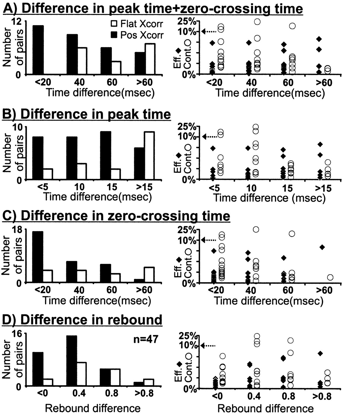
To examine the role of timing in geniculocortical connectivity, we measured the response time course from all cell pairs that met two criteria. First, the geniculate center overlapped a simple-cell subregion of the same sign (n = 104). Second, the geniculate center overlapped the cortical subregion in a near-optimal position (relative overlap > 50%, n = 47; see Materials and Methods; Fig. 5A). All these cell pairs had a high probability of being monosynaptically connected because of the precise match in receptive-field position and sign (31 of 47 were connected). The distributions of peak time, zero-crossing time, and rebound index from these cell pairs were very similar to the distributions from the entire sample (Fig. 7; see also Fig. 10 legend). The selected cell pairs included both presumed directional (predicted DI > 0.3, see Materials and Methods; 12/20 connected) and nondirectional (19/27 connected) simple cells. Most geniculate cells had small receptive fields (less than two simple-cell subregion widths; see Receptive-field sign), although five cells with larger receptive fields were also included (three connected). From the 47 cell pairs used in this analysis, those with similar response time courses had a higher probability of being connected (Fig. 10). In particular, cell pairs that had both similar peak time and zero-crossing time were all connected (n = 12; Fig. 10A). Directionally selective simple cells were included in all timing groups. For example, in Figure 10A there were four, five, two, and one directionally selective cells in the time groups <20, 40, 60, and >60 msec, respectively. Similar results were obtained if we restricted our sample to geniculate centers overlapped with the dominant subregion of the simple cell (n = 31). Interestingly, the efficacy and contributions of the connections seemed to depend little on the relative timing of the visual responses (Fig. 10, right).

View larger version (53K): [in this window] [in a new window]   Figure 10.   Distribution of timing differences between geniculate cells and simple cells among connected and nonconnected cell pairs. Data shown are for cell pairs with well overlapped fields (normalized dot product > 0.50) and impulse responses with good signal to noise (peak  5 SD), selected from all cell pairs with receptive fields of the same sign (n = 47/104). A, All cells with a similar peak time and zero-crossing time were monosynaptically connected. A-C, Differences in timing parameters are shown as absolute values. Geniculate cells were faster than cortical cells in all but two cases (a connected cell pair with peak time + zero-crossing time < 20 msec and a nonconnected cell pair with peak time + zero-crossing time > 60 msec). D, Differences in the rebound index are given as geniculate  cortex. Five of the 47 geniculate cells selected had large receptive fields (most likely Y cells). Timing differences for the three connected large cells are as follows (peak time + zero-crossing time, peak time, zero-crossing time, rebound index): 23, 11, 12, 0.1; 48, 13, 35, 1.1; and 56, 17, 39, 1.1. Timing differences for the two unconnected large cells are as follows: 79, 17, 62, 0.8; and 186, 26, 160, 0.3. The distributions of peak time, zero-crossing time, and rebound index from the selected cell pairs were very similar to the distributions from the entire sample: for selected cell pairs (geniculate cell, simple cell), peak time (27.38 ± 5.88 msec, 37.85 ± 10.90 msec), zero-crossing time (51.20 ± 9.71 msec, 77.06 ± 24.75 msec), and rebound index (0.87 ± 0.30, 0.74 ± 0.46); and for the entire sample (geniculate cell, simple cell), peak time (27.63 ± 8.65 msec, 38.07 ± 11.00 msec), zero-crossing time (50.54 ± 17.25 msec, 79.77 ± 26.89 msec), and rebound index (0.86 ± 0.31, 0.56 ± 0.53). Conventions are as described in Figures 3 and 4.

Although our sample of them was quite small, lagged cells are of considerable interest and therefore deserve comment. We recorded from 13 potentially lagged LGN cells whose centers were superimposed with a simple-cell subregion (eight with rebound indices between 1.2 and 1.5; five with rebound indices >1.9). Only seven of these pairs could be used for timing comparisons (in one pair the baseline of the correlogram had insufficient spikes; in three pairs the geniculate receptive fields were very large; in two cell pairs the geniculate centers were at the border between subregions). Of these seven cell pairs, three were fortuitously superimposed with same-signed "lagged-like" cortical subregions (rebound indices > 1.0). All three of these pairs were connected.

The centers of the remaining four potentially lagged geniculate cells overlapped cortical subregions that were not lagged-like (rebound indices < 1.0). The sign of the overlap in these cases is ambiguous, because it depends on whether the first phase of the geniculate impulse response (our convention) or the second phase (which corresponds to the lagged response) is used. When the first phase of the geniculate response matched the first phase of the cortical response (only one case), the cells were connected. When the first phases did not match (three cases), the cells were not connected.

In summary, we have three candidate examples in which potentially lagged LGN cells were superimposed with lagged-like cortical subregions, all of which were monosynaptically connected. These few examples are consistent with the hypothesis that the lagged-like responses in cortex are at least partially caused by lagged geniculate input (Saul and Humphrey, 1992). Conversely, when a potentially lagged cell was superimposed over a nonlagged cortical subregion, a connection was found only when the first phases of the responses matched.

Subregion strength

Simple receptive fields usually have one or two strong central subregions flanked by weaker subregions. In addition to the factors described above (receptive-field position, sign, and timing) the probability of finding a monosynaptic connection was higher when the geniculate center overlapped the strongest subregion of the simple cell (as in Figs. 1, 8). This rule was not absolute, however, because we found numerous examples of connected pairs in which the LGN center overlapped a weaker subregion (Fig. 11).

View larger version (17K): [in this window] [in a new window]   Figure 11.   Monosynaptic connection between a geniculate cell and a simple cell. The geniculate center overlaps a simple-cell flank. Left, Middle, The receptive fields for the geniculate cell and the simple cell are shown. The receptive field of the simple cell has a strong OFF subregion and a weaker ON flank (70% of the response of the dominant subregion). Right, The correlogram shows a small but significant positive peak (asterisk) displaced from zero indicating a direct excitatory connection. Number of geniculate spikes in the correlogram: 67,111; number of simple-cell spikes in the correlogram: 29,214. Both receptive fields were plotted at the same delays between stimulus and response (32-52 msec). The stimulus was updated every 20 msec.

We divided simple receptive fields into dominant subregions and flanks based on the location of the stimulus pixel that evoked the strongest response (see Materials and Methods for definition of subregion strength). Flanks were further subdivided into strong flanks (total response, 50-99% of the dominant subregion) and weak flanks (<50% of dominant subregion). We selected for this analysis all cell pairs in which the simple-cell subregion was overlapped by a geniculate center of the same sign (n = 104) and, specifically, by the strongest pixel of the geniculate center (n = 67). Most geniculate cells that were monosynaptically connected overlapped the dominant subregion of the simple cell (n = 26 of 39; Fig. 12). A smaller fraction of cells that overlapped strong flanks were connected (n = 8 of 17), and yet fewer were connected that overlapped weak flanks (n = 4 of 11). For the very weakest flanks studied (<30 of the dominant subregion), none of the four overlapping geniculate cells were connected (data not shown). Similarly, the efficacy and contribution of the connections seemed to be weaker when the geniculate center overlapped a weak flank. These results are consistent with the proposal of Hubel and Wiesel (1962) that the weakest subregions result from the surrounds of geniculate cells, whereas moderately strong flanking subregions might result from a combination of geniculate centers and surrounds. This idea is further supported by the finding that the weakest subregions tend to have responses with slower time courses, similar to those of the geniculate surrounds (e.g., Fig. 8). Thus it seems likely that simple cells with one dominant subregion and two weak flanks are built by a single row of geniculate centers, whereas simple cells with two strong subregions (i.e., one dominant and one strong flank) originate from two rows of geniculate centers.

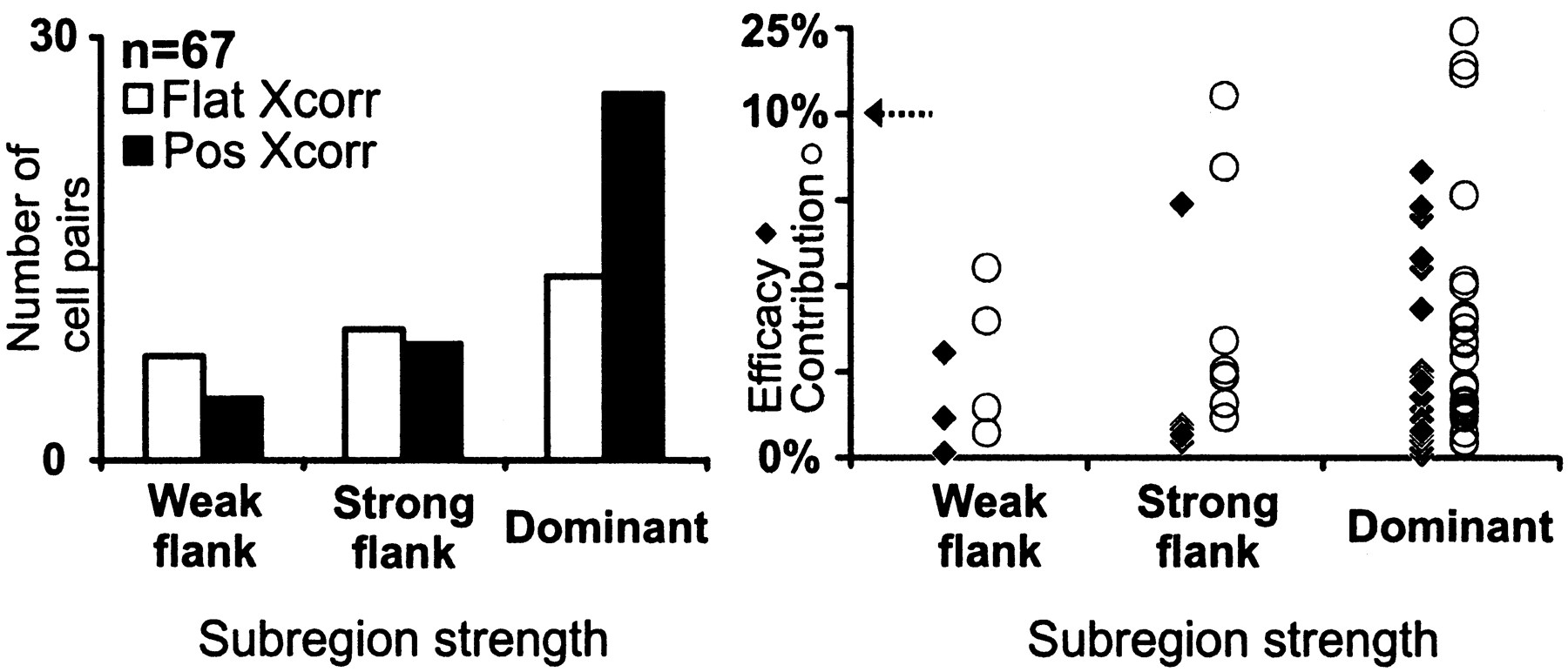
View larger version (19K): [in this window] [in a new window]   Figure 12.   Distribution of connected and nonconnected cell pairs as a function of the response strength from the overlapped simple-cell subregion. We selected only cell pairs in which the strongest pixel of the geniculate receptive field overlapped a pixel of a same-sign simple-cell subregion (n = 67). The dominant subregion is the strongest subregion within the simple receptive field. The strong flank is 50-99% of the response of the dominant subregion. The weak flank is <50% of the response of the dominant subregion.

Receptive-field size

The probability of finding a monosynaptic connection between a geniculate cell and a simple cell was higher when the diameter of the geniculate center matched or was slightly larger than the width of the simple-cell subregion (Figs. 1, 8, 11) (see also Reid and Alonso, 1995; Alonso et al., 1996). Exceptions to this rule, however, were not uncommon, particularly for cells with large receptive fields.

A simultaneous recording from three cells, which illustrates both the rule and the exception, is shown in Figure 13. In this example, the large center of a geniculate cell was overlapped with a large simple-cell subregion of the same sign (cell A), and as would be expected, a strong positive peak was observed in the correlogram. The same geniculate center, however, overlapped both the ON and the OFF subregions of another simple cell (cell B), and still a positive peak was found. The exception represented by the connection to simple cell B in Figure 13 demonstrates that cross-correlation analysis can detect some weak connections between cells with receptive fields of different sign (ON overlapped with OFF).

View larger version (35K): [in this window] [in a new window]   Figure 13.   Two neighboring simple cells receive input from a common Y geniculate cell. A very large geniculate receptive field overlaps a subregion of the same sign in cell A, but it also overlaps both ON and OFF subregions in cell B. The cell is presumably a Y cell because its center is >2.5 times the width of the subregions of the cortical receptive fields (Stoelzel et al., 2000; Yeh et al., 2000). The two simple cells were recorded with the same electrode. The asterisk indicates a significant monosynaptic peak (see Materials and Methods). Number of spikes: geniculate cell, 12,321; simple cell A, 26,192; simple cell B, 1671. All receptive fields were plotted at the same delays between stimulus and response (32-52 msec). The stimulus was updated every 20 msec.

Although the diameter of most geniculate centers approximately matched the width of the overlapped simple-cell subregion, many cells had receptive fields that were twice or three times as large. The relationship between relative size and connectivity is shown in Figure 14 for the subset of cells with the same sign. This figure illustrates our fifth rule of connectivity: the probability of finding a monosynaptic connection was highest when the diameter of the geniculate center was similar or slightly larger than the subregion width. The size rule, however, was our least strict rule. For example, strong connections were sometimes found between cells with different receptive-field sizes (Fig. 14, right). In general, however, connections with large efficacy and contribution were usually found when the geniculate center mostly overlapped a subregion of the same sign (Fig. 13, cell A).

View larger version (17K): [in this window] [in a new window]   Figure 14.   Distribution of connected and nonconnected cell pairs as a function of the relative sizes of the receptive fields. Left, Number of connected (positive cross-correlation) and nonconnected (flat cross-correlation) cell pairs as a function of relative receptive-field size for pairs with same-sign overlapped subregions (n = 104) is shown. Right, The probability of finding a monosynaptic connection was slightly higher when the geniculate center was similar to or slightly larger than the simple-cell subregion (ratio, 1-1.5). Conventions are as described in Figures 3 and 4.

All size measurements were performed by fitting geniculate receptive fields to a symmetric two-dimensional Gaussian function, but it is worth noting that some of our geniculate receptive fields were somewhat elongated, as reported in previous studies (Daniels et al., 1977; Vidyasagar and Urbas, 1982; Schall et al., 1986; Soodak et al., 1987; Cai et al., 1997). It has been suggested that these slight receptive-field asymmetries may play a role in the generation of orientation selectivity (Vidyasagar and Urbas, 1982). Unfortunately, this hypothesis could not be tested in our study because of the relatively small sample of clearly elongated geniculate receptive fields.

	DISCUSSION

TOP ABSTRACT INTRODUCTION MATERIALS AND METHODS RESULTS DISCUSSION REFERENCES

We examined the specificity of connections between pairs of cells in the LGN and visual cortex of the cat. The probability of finding a connection was highest when cell pairs were similar in terms of five receptive-field parameters: (1) sign, (2) position, (3) timing, (4) subregion strength, and (5) size. Previous work has shown that receptive-field position and sign are extremely important (see also Tanaka, 1983, 1985; Reid and Alonso, 1995). Here, we have built on this finding with a larger data set and also demonstrated that the probability of finding a connection depends on response timing, subregion strength, and receptive-field size. In addition, we have demonstrated that the strength of connections (efficacy and contribution) depends on the similarity between the geniculate and cortical receptive fields.

Timing of simple-cell subregions

The overwhelming majority of our geniculate cells were nonlagged, but even within this population there was a broad range of response timing. This range was even broader among the overlapped cortical subregions (Fig. 7). Our data indicate that the connections between geniculate cells and simple cells are predominantly found when both cells respond with similar time courses. This result suggests that two geniculate cells with overlapping receptive fields but different response timing would not converge onto the same simple cell. An interesting consequence of this finding relates to directionally selective simple cells. These cells have different time courses of response at different positions within the receptive field, a characteristic known as spatiotemporal inseparability (Movshon et al., 1978; Adelson and Bergen, 1985; Reid et al., 1987, 1991; McLean and Palmer, 1989; DeAngelis et al., 1993a,b; Jagadeesh et al., 1993, 1997). On the basis of the resemblance between the range of response dynamics within cortical receptive fields and the dynamics of different classes of geniculate cells (lagged and nonlagged), Saul and Humphrey (1992) suggested that some simple cells could receive convergent input from geniculate cells with a range of response dynamics. Our results are consistent with this hypothesis, although they do not prove all aspects of it. Most monosynaptic connections were found between cell pairs for which the geniculate center matched the timing of the overlapped portion of the simple receptive field (peak time, zero-crossing time, and relative strength of the rebound). These results provide strong support for a weaker version of the hypothesis, which concerns mainly nonlagged cells and partially lagged cells.

For lagged cells, our evidence is more anecdotal. In three examples, when the geniculate center and the superimposed cortical subregion were of the same sign and both had a lagged-like signature (rebound > peak), a connection was found. In four other examples, in which the geniculate center was lagged-like and the cortical subregion was nonlagged-like (peak > rebound), a connection was found only when the peaks had the same sign.

Receptive-field size

Our fifth rule of connectivity, that the diameter of the geniculate center tends to be equal to (or slightly larger than) the width of the simple-cell subregion (Fig. 14), was the weakest of the five rules we examined. In particular, the most notable exception to like-to-like connectivity rules was seen in the connections made by geniculate cells with large receptive fields (Figs. 3B, 13, 14). By definition (see Materials and Methods), the receptive-field centers of these cells were more than two times larger than the width of the overlapped simple-cell subregion. Consequently, these receptive fields usually overlapped simple-cell subregions of one sign and portions of adjacent subregions of the opposite sign. When the position of their peak response was considered, however, these geniculate cells nevertheless obeyed the sign rule; monosynaptic connections were more common when there was same-sign overlap (Fig. 3B).

Many studies proposed that X and Y geniculate axons are either entirely (Ferster and LeVay, 1978; Gilbert and Wiesel, 1979) or partially (Freund et al., 1985a; Humphrey et al., 1985) segregated within layer 4 and usually drive different cortical neurons (Bullier and Henry, 1979a,b; Ferster and Lindstrom, 1983; Tanaka, 1983; Martin and Whitteridge, 1984; Mullikin et al., 1984; Freund et al., 1985b). Our size rule is only weakly consonant with these findings, so we can only draw limited conclusions. We did not systematically compare the relative sizes of cortical receptive fields in a given penetration. We also did not explicitly identify geniculate cells on the basis of their response linearity, although most cells within our group of large receptive fields are very likely to be Y cells (Stoelzel et al., 2000; Yeh et al., 2000). Therefore, although our results on the relative sizes of geniculate and cortical receptive fields (Fig. 14) are suggestive, we cannot offer definitive proof that X cells preferentially target cortical cells with small receptive fields and Y cells target those with larger receptive fields.

Certainly, examples of connections from geniculate cells with large receptive fields, noted above, argue for some mixing of the X and Y pathways. More directly, some simple cells have been shown to receive convergent input from geniculate cells with receptive fields of very different size [particularly when the simple cell has both a small and large subregion; Alonso et al. (1996), their Fig. 4; Tanaka (1983), his Fig. 5]. It remains unclear whether this partial X-Y mixing is produced by "developmental mistakes" or whether it has some functional significance.

Number of geniculate inputs to a simple cell

In the present study we examined the probability of finding a connection between individual geniculate and cortical neurons, given their receptive fields. The following question remains: how many geniculate cells converge onto a simple cell? Tanaka (1983) made an estimate of this number based on the strength of cross-correlations he measured between geniculocortical pairs. On average, he found that 10% of the spikes produced by a simple cell fell within the peak of its correlogram with a single geniculate cell. Assuming that simple-cell responses are dominated by geniculate inputs, he estimated that 10 geniculate cells converge onto a single target. Tanaka's estimates encounter several objections. First, his measurements overestimated the real contribution from a single geniculate input because geniculate cells are themselves strongly correlated (Alonso et al., 1996). This overestimation is perhaps compounded by the fact that his integration window to quantify the strength of monosynaptic peaks was broader than that used here. Second, it assumed that all cortical spikes are "caused" in some direct sense by geniculate spikes, which may not be the case because most excitatory connections come from intracortical sources (LeVay and Gilbert, 1976; Peters and Payne, 1993; Ahmed et al., 1994; but see Ferster et al., 1996).

The number of geniculate cells converging onto a cortical cell can also be estimated on the basis of anatomical grounds. It has been calculated that there are 125 total geniculocortical synapses on any given layer 4 spiny stellate cell in area 17 (Peters and Payne, 1993). Freund et al. (1985b) counted the number of synapses made by geniculate axons onto visual cortical neurons and found only one synapse in most cases, with a maximum of eight. From this very small sampling, the number of different thalamic afferents that converge onto a cortical target could therefore range between the extreme values of 15 and 125.

Finally, another estimate of the geniculocortical convergence can be based on a combination of anatomical data from the literature and physiological data from the current study. The number of geniculate inputs converging onto a simple cell can be obtained via the following equation: N = A^.C^.p, where A is the minimum number of geniculate centers that cover a simple receptive field (that is, the area of a simple receptive field relative to a geniculate center), C is the coverage factor (number of geniculate centers per point of visual space), and p is the probability that a geniculate cell and a simple cell with overlapping receptive fields are connected. An average layer 4 simple cell has two to three subregions, each with a length/width ratio of ~2.5 (Fig. 4D). Therefore, six geniculate receptive fields would suffice to cover a simple receptive field. The coverage factor for X cells (ON and OFF combined) is approximately six in the retina (Wässle et al., 1981) and 2.5 times larger in the LGN (see Peters and Payne, 1993); therefore, C = 15. The probability of finding a monosynaptic connection between a geniculate cell and a simple cell with overlapping receptive fields is approximately one-third, from the current study. Thus, ~30 geniculate cells would converge onto a simple cell (N = 6^.15^.0.33).

Although simple receptive fields are approximately outlined by this small set of highly specific geniculocortical afferents, they are also likely to be shaped by intracortical processing, both excitatory and inhibitory. Certainly, geniculate afferents are outnumbered by excitatory intracortical connections (LeVay and Gilbert, 1976; Peters and Payne, 1993; Ahmed et al., 1994). Moreover, inhibition plays an important role in generating response properties of cortical neurons (Sillito, 1992). Along these lines, recent intracellular studies have validated the previous idea that simple-cell subregions are formed by a push-pull mechanism: ON excitation superimposed with OFF inhibition and vice versa (Hubel and Wiesel, 1962; Palmer and Davis, 1981; Ferster, 1988; Tolhurst and Dean, 1990; Hirsch et al., 1998; but see Borg-Graham et al., 1998).

In summary, our results demonstrate that there is a high specificity in the connections between simple cells and their geniculate inputs. These connections follow rules similar to those of the connections from retinal afferents to geniculate cells (Hubel and Wiesel, 1961; Cleland et al., 1971a,b; Kaplan and Shapley, 1984; Kaplan et al., 1987; Mastronarde, 1987b, 1992; Usrey and Reid, 1999). Taken together, these results emphasize the remarkable precision of the developmental mechanisms that determine the feedforward connections in the retinogeniculocortical pathway.

	FOOTNOTES

Received Dec. 15, 2000; revised March 8, 2001; accepted March 13, 2001.

This research was supported by National Institutes of Health Grants R01 EY10115 and EY05253, The Klingenstein Fund, Fulbright/Ministerio de Educación y Ciencia, and by the Charles Revson Foundation. We thank T. N. Wiesel for insightful discussion and invaluable suggestions at all stages of this project. Thanks to two anonymous reviewers for helping to improve this manuscript. Expert technical assistance was provided by Kathleen McGowan.

Correspondence should be addressed to Dr. Jose-Manuel Alonso, Department of Psychology, University of Connecticut, Storrs, CT 06269. E-mail: alonso{at}uconnvm.uconn.edu.

	REFERENCES

TOP ABSTRACT INTRODUCTION MATERIALS AND METHODS RESULTS DISCUSSION REFERENCES

• Adelson EH, Bergen JR (1985) Spatiotemporal energy models for the perception of motion. J Opt Soc Am 2:284-299[Web of Science][Medline].
• Ahmed B, Anderson JC, Douglas RJ, Martin KAC, Nelson JC (1994) Polyneuronal innervation of spiny stellate neurons in cat visual cortex. J Comp Neurol 341:39-49[Web of Science][Medline].
• Alonso JM, Martinez LM (1998) Functional connectivity between simple cells and complex cells in cat striate cortex. Nat Neurosci 1:395-403[Web of Science][Medline].
• Alonso JM, Usrey WM, Reid EC (1996) Precisely correlated firing in cells of the lateral geniculate nucleus. Nature 383:815-819[Medline].
• Borg-Graham LJ, Monier C, Fregnac Y (1998) Visual input evokes transient and strong shunting inhibition in visual cortical neurons. Nature 393:369-373[Medline].
• Bullier J, Henry GH (1979a) Neuronal path taken by afferent streams in striate cortex of the cat. J Neurophysiol 42:1264-1270[Free Full Text].
• Bullier J, Henry GH (1979b) Laminar distribution of first-order neurons and afferent terminals in cat striate cortex. J Neurophysiol 42:1271-1281[Free Full Text].
• Bullier J, Mustari MJ, Henry GH (1982) Receptive-field transformations between LGN neurons and S-cells of cat-striate cortex. J Neurophysiol 47:417-438[Free Full Text].
• Cai D, DeAngelis GC, Freeman RD (1997) Spatiotemporal receptive field organization in the lateral geniculate nucleus of cats and kittens. J Neurophysiol 78:1045-1061[Abstract/Free Full Text].
• Changeux JP, Danchin A (1976) Selective stabilization of developing synapses as a mechanism for the specification of neuronal networks. Nature 264:705-711[Medline].
• Chung S, Ferster D (1998) Strength and orientation tuning of the thalamic input to simple cells revealed by electrically evoked cortical suppression. Neuron 20:1177-1189[Web of Science][Medline].
• Cleland BG, Dubin MW, Levick WR (1971a) Sustained and transient neurones in the cat's retina and lateral geniculate nucleus. J Physiol (Lond) 217:473-496[Abstract/Free Full Text].
• Cleland BG, Dubin MW, Levick WR (1971b) Simultaneous recording of input and output of lateral geniculate neurones. Nat New Biol 231:191-192[Web of Science][Medline].
• Daniels JD, Norman JL, Pettigrew JD (1977) Biases for oriented moving bars in lateral geniculate nucleus neurons of normal and stripe-reared cats. Exp Brain Res 29:155-172[Web of Science][Medline].
• DeAngelis GC, Ohzawa I, Freeman RD (1993a) Spatiotemporal organization of simple-cell receptive fields in the cat's striate cortex. I. General characteristics and postnatal development. J Neurophysiol 69:1091-1117[Abstract/Free Full Text].
• DeAngelis GC, Ohzawa I, Freeman RD (1993b) Spatiotemporal organization of simple-cell receptive fields in the cat's striate cortex. II. Linearity of temporal and spatial summation. J Neurophysiol 69:1118-1135[Abstract/Free Full Text].
• Eckhorn R, Thomas U (1993) Guidance of thin-shaft microprobes by rubber tubes: a new method for the insertion of multiple microprobes into neural and muscular tissue, including fiber-electrodes, fine wires, needles and microsensors. J Neurosci Methods 49:175-185[Web of Science][Medline].
• Enroth-Cugell C, Robson JG (1966) The contrast sensitivity of retinal ganglion cells of the cat. J Physiol (Lond) 187:517-552.
• Ferster D (1988) Spatially opponent excitation and inhibition in simple cells of the cat visual cortex. J Neurosci 8:1172-1180[Abstract].
• Ferster D, LeVay S (1978) The axonal arborizations of lateral geniculate nucleus in the striate cortex of the cat. J Comp Neurol 182:923-944[Web of Science][Medline].
• Ferster D, Lindstrom S (1983) An intracellular analysis of geniculo-cortical connectivity in area 17 of the cat. J Physiol (Lond) 342:181-215[Abstract/Free Full Text].
• Ferster D, Chung S, Wheat H (1996) Orientation selectivity of thalamic input to simple cells of cat visual cortex. Nature 380:249-252[Medline].
• Freund TF, Martin KAC, Whitteridge D (1985a) Innervation of cat visual areas 17 and 18 by physiologically identified X- and Y-type thalamic afferents. I. Arborization patterns and quantitative distribution of postsynaptic elements. J Comp Neurol 242:263-274[Web of Science][Medline].
• Freund TF, Martin KAC, Somogyi P, Whitteridge D (1985b) Innervation of cat visual areas 17 and 18 by physiologically identified X- and Y-type thalamic afferents. II. Identification of postsynaptic targets by GABA immunocytochemistry and Golgi impregnation. J Comp Neurol 242:275-291[Web of Science][Medline].
• Gardner JL, Anzai A, Ohzawa I, Freeman RD (1999) Linear and nonlinear contributions to orientation tuning of simple cells in the cat's striate cortex. Vis Neurosci 16:1115-1121[Web of Science][Medline].
• Gielen CCAM, van Gisbergen JAM, Vendrik AJH (1982) Reconstruction of cone-system contributions to responses of colour-opponent neurones in monkey lateral geniculate. Biol Cybern 44:211-221[Web of Science][Medline].
• Gilbert CD, Wiesel TN (1979) Morphology and intracortical projections of functionally characterized neurons in the cat visual cortex. Nature 280:120-125[Medline].
• Goodman CS, Shatz CJ (1993) Developmental mechanisms that generate precise patterns of neuronal connectivity. Cell 72:77-98.
• Hirsch JA, Alonso JM, Reid RC, Martinez LM (1998) Synaptic integration in the simple receptive field. J Neurosci 18:9517-9528[Abstract/Free Full Text].
• Hochstein S, Shapley RM (1976) Quantitative analysis of retinal ganglion cell classification. J Physiol (Lond) 262:237-264[Abstract/Free Full Text].
• Hoffmann KP, Stone J, Sherman SM (1972) Relay of receptive-field properties in dorsal lateral geniculate nucleus of the cat. J Neurophysiol 35:518-531[Free Full Text].
• Hubel DH, Wiesel TN (1961) Integrative action in the cat's lateral geniculate body. J Physiol (Lond) 155:385-398.
• Hubel DH, Wiesel TN (1962) Receptive fields, binocular interaction and functional architecture in the cat's visual cortex. J Physiol (Lond) 160:106-154.
• Humphrey AL, Weller RE (1988) Functionally distinct groups of X-cells in the lateral geniculate nucleus of the cat. J Comp Neurol 233:159-189.
• Humphrey AL, Sur M, Ulrich DJ, Sherman SM (1985) Projection patterns of individual X- and Y-cell axons from the lateral geniculate nucleus to cortical area 17 in the cat. J Comp Neurol 233:159-189[Web of Science][Medline].
• Jagadeesh B, Wheat HS, Ferster D (1993) Linearity of summation of synaptic potentials underlying direction selectivity in simple cells of the cat visual cortex. Science 262:1901-1904[Abstract/Free Full Text].
• Jagadeesh B, Wheat HS, Kontsevich LL, Tyler CW, Ferster D (1997) Direction selectivity of synaptic potentials in simple cells of the cat visual cortex. J Neurosci 78:2772-2789.
• Jones JP, Palmer LA (1987) The two-dimensional spatial structure of simple receptive fields in cat striate cortex. J Neurophysiol 58:1187-1211[Abstract/Free Full Text].
• Jones JP, Stepnoski A, Palmer LA (1987) The two-dimensional spectral structure of simple receptive fields in cat striate cortex. J Neurophysiol 58:1212-1232[Abstract/Free Full Text].
• Kaplan E, Shapley R (1984) The origin of the S (slow) potential in the mammalian lateral geniculate nucleus. Exp Brain Res 55:111-116[Web of Science][Medline].
• Kaplan E, Purpura K, Shapley RM (1987) Contrast affects the transmission of visual information through the mammalian lateral geniculate nucleus. J Physiol (Lond) 391:267-288[Abstract/Free Full Text].
• LeVay S, Gilbert CD (1976) Laminar patterns of geniculocortical projection in the cat. Brain Res 113:1-19[Web of Science][Medline].
• Levick WR, Cleland BG, Dubin MW (1972) Lateral geniculate neurons of cat: retinal inputs and physiology. Invest Ophthalmol 11:302-311[Abstract/Free Full Text].
• Lu SM, Guido W, Vaughan JW, Sherman SM (1995) Latency variability of responses to visual stimuli in cells of the cat's lateral geniculate nucleus. Exp Brain Res 105:7-17[Web of Science][Medline].
• Marcelja S (1980) Mathematical description of the responses of simple cortical cells. J Opt Soc Am 70:1297-1300[Medline].
• Martin KAC, Whitteridge D (1984) Form, function and intracortical projections of spiny neurons in the striate visual cortex of the cat. J Physiol (Lond) 353:463-504[Abstract/Free Full Text].
• Martinez LM, Reid RC, Alonso JM, Hirsch JA (1999) The synaptic structure of the simple receptive field. Soc Neurosci Abstr 25:1048.
• Mastronarde DN (1987a) Two classes of single-input X-cells in cat lateral geniculate nucleus. I. Receptive-field properties and classification of cells. J Neurophysiol 57:357-380[Abstract/Free Full Text].
• Mastronarde DN (1987b) Two classes of single-input X-cells in cat lateral geniculate nucleus. II. Retinal inputs and the generation of receptive field properties. J Neurophysiol 57:381-413[Abstract/Free Full Text].
• Mastronarde DN (1992) Nonlagged relay cells and interneurons in the cat lateral geniculate nucleus: receptive-field properties and retinal inputs. Vis Neurosci 8:407-441[Web of Science][Medline].
• McLean J, Palmer LA (1989) Contribution of linear spatiotemporal field structure to velocity selectivity of simple cells in area 17 of cat. Vision Res 29:675-679[Web of Science][Medline].
• Miller KD (1994) A model for the development of simple cell receptive fields and the ordered arrangement of orientation columns through activity-dependent competition between ON- and OFF-center inputs. J Neurosci 14:409-441[Abstract].
• Miller KD, Keller JB, Stryker MP (1989) Ocular dominance column development: analysis and simulation. Science 245:605-615[Abstract/Free Full Text].
• Movshon JA, Thompson ID, Tolhurst DJ (1978) Spatial summation in the receptive field of simple cells in the cat's striate cortex. J Physiol (Lond) 283:53-77[Abstract/Free Full Text].
• Mullikin WH, Jones JP, Palmer LA (1984) Receptive-field properties and laminar distribution of X-like and Y-like simple cells in cat area 17. J Neurophysiol 52:350-371[Abstract/Free Full Text].
• Palmer LA, Davis TL (1981) Receptive field structure in cat striate cortex. J Neurophysiol 46:260-276[Free Full Text].
• Pei X, Vidyasagar TR, Volgushev M, Creutzfeldt OD (1994) Receptive field analysis and orientation selectivity of postsynaptic potentials of simple cells in cat visual cortex. J Neurosci 14:7130-7140[Abstract].
• Perkel DH, Gerstein GL, Moore GP (1967) Neuronal spike trains and stochastic point processes. II. Simultaneous spike trains. Biophys J 7:419-440.
• Peters A, Payne BR (1993) Numerical relationships between geniculocortical afferents and pyramidal cell modules in cat primary visual cortex. Cereb Cortex 3:69-78[Abstract/Free Full Text].
• Reid RC, Alonso JM (1995) Specificity of monosynaptic connections from thalamus to visual cortex. Nature 378:281-284[Medline].
• Reid RC, Alonso JM (1996) The processing and encoding of information in the visual cortex. Curr Opin Neurobiol 6:475-480[Web of Science][Medline].
• Reid RC, Shapley RM (1992) Spatial structure of cone inputs to receptive fields in primate lateral geniculate nucleus. Nature 356:716-717[Medline].
• Reid RC, Soodak RE, Shapley RM (1987) Linear mechanisms of directional selectivity in simple cells of cat striate cortex. Proc Natl Acad Sci USA 84:8740-8744[Abstract/Free Full Text].
• Reid RC, Soodak RE, Shapley RM (1991) Directional selectivity and spatiotemporal structure of receptive fields of simple cells in cat striate cortex. J Neurophysiol 66:505-529[Abstract/Free Full Text].
• Reid RC, Victor JD, Shapley RM (1997) The use of m-sequences in the analysis of visual neurons: linear receptive field properties. Vis Neurosci 14:1015-1027[Web of Science][Medline].
• Rodieck RW (1965) Quantitative analysis of cat retinal ganglion cell response to visual stimuli. Vision Res 5:583-601[Medline].
• Saul AB, Humphrey AL (1990) Spatial and temporal response properties of lagged and nonlagged cells in cat lateral geniculate nucleus. J Neurophysiol 64:206-223[Abstract/Free Full Text].
• Saul AB, Humphrey AL (1992) Evidence of input from lagged cells in the lateral geniculate nucleus to simple cells in cortical area 17 of the cat. J Neurophysiol 68:1190-1208[Abstract/Free Full Text].
• Schall JD, Perry VH, Leventhal AG (1986) Retinal ganglion cell dendritic fields in old-world monkeys are oriented radially. Brain Res 368:18-23[Web of Science][Medline].
• Sillito AM (1992) GABA mediated inhibitory processes in the function of the geniculo-striate system. Prog Brain Res 90:349-384[Web of Science][Medline].
• Soodak RE, Shapley RM, Kaplan E (1987) Linear mechanism of orientation tuning in the retina and lateral geniculate nucleus of the cat. J Neurophysiol 58:267-275[Abstract/Free Full Text].
• Stent GS (1973) A physiological mechanism for Hebb's postulate of learning. Proc Natl Acad Sci USA 70:997-1001[Abstract/Free Full Text].
• Stoelzel CR, Yeh CI, Bachand J, Alonso JM (2000) Tight correlated firing between cells in layer C of the cat lateral geniculate nucleus: a comparison with layer A. Soc Neurosci Abstr 26:1965.
• Stryker MP, Strickland SL (1984) Physiological segregation of ocular dominance columns depends on the pattern of afferent electrical activity. Invest Ophthalmol Vis Sci [Suppl] 25:278[Abstract/Free Full Text].
• Sutter EE (1992) A deterministic approach to nonlinear systems analysis. In: Nonlinear vision: determination of neural receptive fields, function and networks (Pinter R, Nabet B, eds), pp 171-220. Cleveland, OH: CRC.
• Swadlow HA (1995) Influence of VPM afferents on putative inhibitory interneurons in S1 of the awake rabbit: evidence for cross-correlation, microstimulation, and latencies to peripheral sensory stimulation. J Neurophysiol 73:1584-1599[Abstract/Free Full Text].
• Swadlow HA, Lukatela K (1996) Cross-correlation and microstimulation: complementary tools in the extracellular analysis of synaptic interactions. J Neurosci Methods 64:219-225[Web of Science][Medline].
• Tanaka K (1983) Cross-correlation analysis of interneural activity in cat visual cortex. J Neurophysiol 49:1301-1318.
• Tanaka K (1985) Organization of geniculate inputs to visual cortical cells in the cat. Vision Res 25:357-364[Web of Science][Medline].
• Tolhurst DJ, Dean AF (1990) The effects of contrast on the linearity of spatial summation of simple cells in the cat's striated cortex. Exp Brain Res 79:582-588[Web of Science][Medline].
• Tusa RJ, Palmer LA, Rosenquist AC (1978) The retinotopic organization of area 17 (striate cortex) in the cat. J Comp Neurol 177:213-236[Web of Science][Medline].
• Usrey WM, Reid RC (1999) Synchronous activity in the visual system. Annu Rev Physiol 61:435-456[Web of Science][Medline].
• Usrey WM, Reid RC (2000) Visual physiology of the lateral geniculate nucleus in two species of New World monkeys: Saimiri sciureus and Aotus trivirgatis. J Physiol (Lond) 523:755-769[Abstract/Free Full Text].
• Usrey WM, Reppas JB, Reid RC (1999) Specificity and strength of retinogeniculate connections. J Neurophysiol 82:3527-3540[Abstract/Free Full Text].
• Usrey WM, Alonso J-M, Reid RC (2000) Synaptic interactions between thalamic inputs to simple cells in cat visual cortex. J Neurosci 20:5461-5467[Abstract/Free Full Text].
• Vidyasagar TR, Urbas JV (1982) Orientation sensitivity of cat LGN neurones with and without inputs from visual cortical areas 17 and 18. Exp Brain Res 46:157-169[Web of Science][Medline].
• Wässle H, Boycott BB, Illing RB (1981) Morphology and mosaic of on- and off-beta cells in the cat retina and some functional considerations. Proc R Soc Lond B Biol Sci 212:177-195[Medline].
• Weliky M, Katz LC (1997) Disruption of orientation tuning in visual cortex by artificially correlated neuronal activity. Nature 386:680-685[Medline].
• Wolfe J, Palmer LA (1998) Temporal diversity in the lateral geniculate nucleus of cat. Vis Neurosci 15:653-675[Web of Science][Medline].
• Yeh CI, Stoelzel CR, Bachand J, Alonso JM (2000) Tight correlated firing is scarce between pairs of layer A-layer C cells of the cat lateral geniculate nucleus. Soc Neurosci Abstr 26:1965.

---

Copyright © 2001 Society for Neuroscience  0270-6474/01/21114002-14$05.00/0

This article has been cited by other articles:

				N. M. da Costa and K. A. C. Martin Selective Targeting of the Dendrites of Corticothalamic Cells by Thalamic Afferents in Area 17 of the Cat J. Neurosci., November 4, 2009; 29(44): 13919 - 13928. [Abstract] [Full Text] [PDF]

				M. Stimberg, K. Wimmer, R. Martin, L. Schwabe, J. Marino, J. Schummers, D. C. Lyon, M. Sur, and K. Obermayer The Operating Regime of Local Computations in Primary Visual Cortex Cereb Cortex, September 1, 2009; 19(9): 2166 - 2180. [Abstract] [Full Text] [PDF]

				J.-M. Alonso My recollections of Hubel and Wiesel and a brief review of functional circuitry in the visual pathway J. Physiol., June 15, 2009; 587(12): 2783 - 2790. [Abstract] [Full Text] [PDF]

				X. Huang and S. G. Lisberger Noise Correlations in Cortical Area MT and Their Potential Impact on Trial-by-Trial Variation in the Direction and Speed of Smooth-Pursuit Eye Movements J Neurophysiol, June 1, 2009; 101(6): 3012 - 3030. [Abstract] [Full Text] [PDF]

				C. R. Stoelzel, Y. Bereshpolova, and H. A. Swadlow Stability of Thalamocortical Synaptic Transmission across Awake Brain States J. Neurosci., May 27, 2009; 29(21): 6851 - 6859. [Abstract] [Full Text] [PDF]

				H. E. Halverson, E. M. Hubbard, and J. H. Freeman Stimulation of the lateral geniculate, superior colliculus, or visual cortex is sufficient for eyeblink conditioning in rats Learn. Mem., April 24, 2009; 16(5): 300 - 307. [Abstract] [Full Text] [PDF]

				C.-I Yeh, C. R. Stoelzel, C. Weng, and J.-M. Alonso Functional Consequences of Neuronal Divergence Within the Retinogeniculate Pathway J Neurophysiol, April 1, 2009; 101(4): 2166 - 2185. [Abstract] [Full Text] [PDF]

				J. Cang, L. Wang, M. P. Stryker, and D. A. Feldheim Roles of Ephrin-As and Structured Activity in the Development of Functional Maps in the Superior Colliculus J. Neurosci., October 22, 2008; 28(43): 11015 - 11023. [Abstract] [Full Text] [PDF]

				C. R. Stoelzel, Y. Bereshpolova, A. G. Gusev, and H. A. Swadlow The Impact of an LGNd Impulse on the Awake Visual Cortex: Synaptic Dynamics and the Sustained/Transient Distinction J. Neurosci., May 7, 2008; 28(19): 5018 - 5028. [Abstract] [Full Text] [PDF]

				R. D. Kumbhani, M. J. Nolt, and L. A. Palmer Precision, Reliability, and Information-Theoretic Analysis of Visual Thalamocortical Neurons J Neurophysiol, November 1, 2007; 98(5): 2647 - 2663. [Abstract] [Full Text] [PDF]

				S. S. Shaevitz and F. E. Theunissen Functional Connectivity Between Auditory Areas Field L and CLM and Song System Nucleus HVC in Anesthetized Zebra Finches J Neurophysiol, November 1, 2007; 98(5): 2747 - 2764. [Abstract] [Full Text] [PDF]

				D. L. Rathbun, H. J. Alitto, T. G. Weyand, and W. M. Usrey Interspike Interval Analysis of Retinal Ganglion Cell Receptive Fields J Neurophysiol, August 1, 2007; 98(2): 911 - 919. [Abstract] [Full Text] [PDF]

				S. E. Palmer and K. D. Miller Effects of Inhibitory Gain and Conductance Fluctuations in a Simple Model for Contrast-Invariant Orientation Tuning in Cat V1 J Neurophysiol, July 1, 2007; 98(1): 63 - 78. [Abstract] [Full Text] [PDF]

				P. E. Williams and R. M. Shapley A Dynamic Nonlinearity and Spatial Phase Specificity in Macaque V1 Neurons J. Neurosci., May 23, 2007; 27(21): 5706 - 5718. [Abstract] [Full Text] [PDF]

				E. A. Allen and R. D. Freeman Dynamic spatial processing originates in early visual pathways. J. Neurosci., November 8, 2006; 26(45): 11763 - 11774. [Abstract] [Full Text] [PDF]

				J. Wielaard and P. Sajda Circuitry and the Classification of Simple and Complex Cells in V1 J Neurophysiol, November 1, 2006; 96(5): 2739 - 2749. [Abstract] [Full Text] [PDF]

				S. Nishimoto, T. Ishida, and I. Ohzawa Receptive field properties of neurons in the early visual cortex revealed by local spectral reverse correlation. J. Neurosci., March 22, 2006; 26(12): 3269 - 3280. [Abstract] [Full Text] [PDF]

				Y. Bereshpolova, C. R. Stoelzel, A. G. Gusev, T. Bezdudnaya, and H. A. Swadlow The impact of a corticotectal impulse on the awake superior colliculus. J. Neurosci., February 22, 2006; 26(8): 2250 - 2259. [Abstract] [Full Text] [PDF]

				F. J Veredas, F. J Vico, and J.-M. Alonso Factors determining the precision of the correlated firing generated by a monosynaptic connection in the cat visual pathway J. Physiol., September 15, 2005; 567(3): 1057 - 1078. [Abstract] [Full Text] [PDF]

				B. D. Moore IV, H. J. Alitto, and W. M. Usrey Orientation Tuning, But Not Direction Selectivity, Is Invariant to Temporal Frequency in Primary Visual Cortex J Neurophysiol, August 1, 2005; 94(2): 1336 - 1345. [Abstract] [Full Text] [PDF]

				M. Gur, I. Kagan, and D. M. Snodderly Orientation and Direction Selectivity of Neurons in V1 of Alert Monkeys: Functional Relationships and Laminar Distributions Cereb Cortex, August 1, 2005; 15(8): 1207 - 1221. [Abstract] [Full Text] [PDF]

				J.-M. Alonso and H. A. Swadlow Thalamocortical Specificity and the Synthesis of Sensory Cortical Receptive Fields J Neurophysiol, July 1, 2005; 94(1): 26 - 32. [Abstract] [Full Text] [PDF]

				A. B Saul, P. L Carras, and A. L Humphrey Temporal Properties of Inputs to Direction-Selective Neurons in Monkey V1 J Neurophysiol, July 1, 2005; 94(1): 282 - 294. [Abstract] [Full Text] [PDF]

				S. Nishimoto, M. Arai, and I. Ohzawa Accuracy of Subspace Mapping of Spatiotemporal Frequency Domain Visual Receptive Fields J Neurophysiol, June 1, 2005; 93(6): 3524 - 3536. [Abstract] [Full Text] [PDF]

				C. Weng, C.-I Yeh, C. R. Stoelzel, and J.-M. Alonso Receptive Field Size and Response Latency Are Correlated Within the Cat Visual Thalamus J Neurophysiol, June 1, 2005; 93(6): 3537 - 3547. [Abstract] [Full Text] [PDF]

				J. A. Cardin, L. A. Palmer, and D. Contreras Stimulus-Dependent {gamma} (30-50 Hz) Oscillations in Simple and Complex Fast Rhythmic Bursting Cells in Primary Visual Cortex J. Neurosci., June 1, 2005; 25(22): 5339 - 5350. [Abstract] [Full Text] [PDF]

				H. A. Swadlow, Y. Bereshpolova, T. Bezdudnaya, M. Cano, and C. R. Stoelzel A Multi-Channel, Implantable Microdrive System for Use With Sharp, Ultra-Fine "Reitboeck" Microelectrodes J Neurophysiol, May 1, 2005; 93(5): 2959 - 2965. [Abstract] [Full Text] [PDF]

				Y. Zhang and R. C. Reid Single-neuron responses and neuronal decisions in a vernier task PNAS, March 1, 2005; 102(9): 3507 - 3512. [Abstract] [Full Text] [PDF]

				D. L. Ringach Haphazard Wiring of Simple Receptive Fields and Orientation Columns in Visual Cortex J Neurophysiol, July 1, 2004; 92(1): 468 - 476. [Abstract] [Full Text] [PDF]

				M. R. Peterson, B. Li, and R. D. Freeman The Derivation of Direction Selectivity in the Striate Cortex J. Neurosci., April 7, 2004; 24(14): 3583 - 3591. [Abstract] [Full Text] [PDF]

				W. H. Swanson, J. Felius, and F. Pan Perimetric Defects and Ganglion Cell Damage: Interpreting Linear Relations Using a Two-Stage Neural Model Invest. Ophthalmol. Vis. Sci., February 1, 2004; 45(2): 466 - 472. [Abstract] [Full Text] [PDF]

				L. Tao, M. Shelley, D. McLaughlin, and R. Shapley An egalitarian network model for the emergence of simple and complex cells in visual cortex PNAS, January 6, 2004; 101(1): 366 - 371. [Abstract] [Full Text] [PDF]

				T. Z. Lauritzen and K. D. Miller Different Roles for Simple-Cell and Complex-Cell Inhibition in V1 J. Neurosci., November 12, 2003; 23(32): 10201 - 10213. [Abstract] [Full Text] [PDF]

				L. M. Martinez and J.-M. Alonso Complex Receptive Fields in Primary Visual Cortex Neuroscientist, October 1, 2003; 9(5): 317 - 331. [Abstract] [PDF]

				P. Kara and R. C. Reid Efficacy of Retinal Spikes in Driving Cortical Responses J. Neurosci., September 17, 2003; 23(24): 8547 - 8557. [Abstract] [Full Text] [PDF]

				C.-I Yeh, C. R. Stoelzel, and J.-M. Alonso Two Different Types of Y Cells in the Cat Lateral Geniculate Nucleus J Neurophysiol, September 1, 2003; 90(3): 1852 - 1864. [Abstract] [Full Text] [PDF]

				S. Grossberg and A. Seitz Laminar Development of Receptive Fields, Maps and Columns in Visual Cortex: The Coordinating Role of the Subplate Cereb Cortex, August 1, 2003; 13(8): 852 - 863. [Abstract] [Full Text] [PDF]

				K. A. Razak, L. Huang, and S. L. Pallas NMDA Receptor Blockade in the Superior Colliculus Increases Receptive Field Size Without Altering Velocity and Size Tuning J Neurophysiol, July 1, 2003; 90(1): 110 - 119. [Abstract] [Full Text] [PDF]

				M. S. Livingstone and B. R. Conway Substructure of Direction-Selective Receptive Fields in Macaque V1 J Neurophysiol, May 1, 2003; 89(5): 2743 - 2759. [Abstract] [Full Text] [PDF]

				W. M. Usrey, M. P. Sceniak, and B. Chapman Receptive Fields and Response Properties of Neurons in Layer 4 of Ferret Visual Cortex J Neurophysiol, February 1, 2003; 89(2): 1003 - 1015. [Abstract] [Full Text] [PDF]

				H. A. Swadlow Fast-spike Interneurons and Feedforward Inhibition in Awake Sensory Neocortex Cereb Cortex, January 1, 2003; 13(1): 25 - 32. [Abstract] [Full Text] [PDF]

				J. A. Hirsch Synaptic Physiology and Receptive Field Structure in the Early Visual Pathway of the Cat Cereb Cortex, January 1, 2003; 13(1): 63 - 69. [Abstract] [Full Text] [PDF]

				J. F. Linden and C. E. Schreiner Columnar Transformations in Auditory Cortex? A Comparison to Visual and Somatosensory Cortices Cereb Cortex, January 1, 2003; 13(1): 83 - 89. [Abstract] [Full Text] [PDF]

				R. M. Bruno and D. J. Simons Feedforward Mechanisms of Excitatory and Inhibitory Cortical Receptive Fields J. Neurosci., December 15, 2002; 22(24): 10966 - 10975. [Abstract] [Full Text] [PDF]

				P. Kara, J. S. Pezaris, S. Yurgenson, and R. C. Reid The spatial receptive field of thalamic inputs to single cortical simple cells revealed by the interaction of visual and electrical stimulation PNAS, December 10, 2002; 99(25): 16261 - 16266. [Abstract] [Full Text] [PDF]

				M. Carandini, D. J Heeger, and W. Senn A Synaptic Explanation of Suppression in Visual Cortex J. Neurosci., November 15, 2002; 22(22): 10053 - 10065. [Abstract] [Full Text] [PDF]

				J.-M. Alonso Book Review: Neural Connections and Receptive Field Properties in the Primary Visual Cortex Neuroscientist, October 1, 2002; 8(5): 443 - 456. [Abstract] [PDF]

				H. A. Swadlow, A. G. Gusev, and T. Bezdudnaya Activation of a Cortical Column by a Thalamocortical Impulse J. Neurosci., September 1, 2002; 22(17): 7766 - 7773. [Abstract] [Full Text] [PDF]

				A. B. Saul and J. C. Feidler Development of Response Timing and Direction Selectivity in Cat Visual Thalamus and Cortex J. Neurosci., April 1, 2002; 22(7): 2945 - 2955. [Abstract] [Full Text] [PDF]

This Article Abstract Full Text (PDF) Submit an eLetter Alert me when this article is cited Alert me when eLetters are posted Alert me if a correction is posted Citation Map Services Email this article to a friend Similar articles in this journal Similar articles in Web of Science Similar articles in PubMed Alert me to new issues of the journal Download to citation manager Citing Articles Citing Articles via HighWire Citing Articles via Web of Science (110) Citing Articles via Google Scholar Google Scholar Articles by Alonso, J.-M. Articles by Reid, R. C. Search for Related Content PubMed PubMed Citation Articles by Alonso, J.-M. Articles by Reid, R. C.

Home  |   Search  |   Archive  |   Subscribe  |   Contact  |   Help