

Abstract
We studied neurons in the central visual field representation of the lateral geniculate nucleus (LGN) in macaque monkeys by mapping their receptive fields in space and time. The mapping was performed by reverse correlation of a spike train of a neuron with pseudorandom, binary level stimuli (m-sequence grids). Black and white m-sequence grids were used to map the receptive field for luminance. The locations of receptive field center and surround were determined from this luminance map. To map the contribution of each cone class to the receptive field, we designed red–green or blue–yellow m-sequence grids to isolate the influence of that cone (long, middle, or short wavelength-sensitive: L, M, or S). Magnocellular neurons generally received synergistic input from L and M cones in both the center and the surround. A minority had cone-antagonistic (M–L) input to the surround. Red–green opponent parvocellular neurons received opponent cone input (L+M− or M+L−) that overlapped in space, as sampled by our stimulus grid, but that had somewhat different extents. For example, an L+ center parvocellular neuron would be L+/M− in both center and surround, but the L+ signal would be stronger in the center and the M− signal stronger in the surround. Accordingly, the luminance receptive field would be spatially antagonistic: on-center/off-surround. The space–time maps also characterized LGN dynamics. For example, magnocellular responses were transient, red–green parvocellular responses were more sustained, and blue-on responses were the most sustained for both luminance and cone-isolating stimuli. For all cell types the surround response peaked 8–10 msec later than the center response.
The purpose of our experiments was to investigate the possible roles in color vision of parvocellular and magnocellular neurons in the lateral geniculate nucleus (LGN) ofMacaca fascicularis. Macaques have three types of cone photoreceptor with peak sensitivities at different wavelengths: the L cones at 565 nm, M cones at 535 nm, and S cones at 440 nm (Smith and Pokorny, 1972, 1975; Baylor et al., 1987). The spatial and temporal maps of these photoreceptors to LGN neurons determine the responses of the neurons to color. We sought to answer the following questions: (1) How are cone photoreceptor signals mapped onto individual LGN cells? (2) How is this mapping different, or similar, for parvocellular and magnocellular neurons? (3) What is the time course of responses for magnocellular and parvocellular neurons in both center and surround?
The influence of each cone class on a receptive field of a neuron was measured with a combination of two techniques: m-sequence grids (a form of white noise receptive field mapping) and cone-isolating stimuli (Fig. 1, Stimuli) (Sutter, 1987, 1992; Reid and Shapley, 1992; Reid et al., 1997). Together, these methods yield spatial maps of the responses evoked by each cone class and, further, characterize the time evolution of these responses. Black and white m-sequence grids were used to characterize the conventional receptive field for achromatic stimuli. From these achromatic measurements we estimated the spatial location and extent of the receptive field center and surround. Then the sign, magnitude, and dynamics of the cone signals that provided the input to the center and surround were determined from the cone maps. This enabled us to determine the dynamics of cone inputs to center and surround in magnocellular and parvocellular neurons. This also allowed us to test hypotheses about the cone inputs to receptive field center and surround.

The cone-specific and mixed surround models for red–green opponent parvocellular neurons, specifically L-on/M-off type I neurons [after Reid and Shapley (1992), their Fig. 1].Stimuli, Representations of the binary m-sequence grid stimuli, which are either luminance modulated (between black and white) or chromatically modulated between hues that modulate either L cones or M cones in isolation. For the L-cone stimulus the red is brighter than the mean (on); the green is darker than the mean (off). For the M-cone stimulus the green is brighter (on); the red is darker (off).Model, Diagrammatic representations of receptive fields, color-coded in terms of the cone-isolating stimuli that drive them. In the cone-specific surround model (first row) the L-on center (L+) is opposed by an M-off surround (M−). In the mixed surround model the L-on center is opposed both by M-off and L-off surround (L− and M−). Predicted Results, Spatial weighting functions as mapped with the luminance, L-cone, and M-cone stimuli. Responses are coded in false color: on (+) inred and off (−) in blue. Responses of the center cone type, the L cone, represent the critical test between models. In the cone-specific surround the L-cone responses are exclusively on. In the mixed surround (arrow), the L-cone responses are on-center/off-surround.
Magnocellular neurons in the LGN receive mixed cone inputs to their receptive field centers and, in most cases, to their surrounds. By contrast, we found direct evidence for the idea that excitation and inhibition in almost all red–green opponent parvocellular neurons (within 13° of the fovea) are both cone-specific. Mixed cone input to the surround would be observable experimentally as an antagonistic center/surround relationship for a single cone class, specifically the cone class of the center (see Fig. 1, arrow). Most red–green opponent parvocellular neurons had center/surround antagonistic responses to a luminance stimulus (type I cells; Wiesel and Hubel, 1966), but the spatial map of cone-isolated responses was monophasic, with a profile resembling a bell-shaped curve. It would be difficult to prove the surround absolutely specific, but our results are consistent with others (Lee et al., 1998) in finding the random-surround model very improbable.
The time course of cone signals is also important for color vision. The dynamics of parvocellular and magnocellular neurons differ for both black and white and cone-isolating stimuli: for all stimuli the magnocellular responses are more transient. Another dynamic result is that surround signals are slower than center signals for magnocellular and red–green opponent parvocellular neurons and for their cone-isolated inputs. As discussed below, this probably is not caused by processes within the LGN but, instead, arises from the properties of retinal circuitry and synapses.
MATERIALS AND METHODS
Cynomolgus monkeys, M. fascicularis(n = 5), were anesthetized initially with ketamine (10 mg/kg, i.m.) and intravenous sodium thiamylal (25 mg/kg, supplemented as needed) and maintained in an anesthetized state during the experiment with urethane (20–30 mg/kg per hr, i.v.). Temperature, EKG, EEG, blood pressure, and expired CO2 were monitored continuously throughout the experiment. Eyes were dilated with 1% atropine and were protected with contact lenses with a 3 mm artificial pupil. The animals were paralyzed with gallamine triethiodide (20–40 mg/hr, i.v.). To minimize residual eye movements under paralysis, we fixed metal posts to the scleras just beyond the limbus with cyanoacrylate glue. Refractive errors were corrected to within one-half diopter with lenses placed in front of the eyes. Lenses were chosen by optimizing the response of a parvocellular neuron to an achromatic drifting grating of high spatial frequency.
Action potentials of neurons in the LGN were recorded with glass-coated tungsten microelectrodes (Alan Ainsworth, London, UK). The Discovery software package (DataWave Systems, Longmont, CO) was used to discriminate the spikes of individual neurons. In some cases two neurons were recorded simultaneously from the same electrode and were discriminated by their amplitude and waveform. Distinctions between magnocellular and parvocellular neurons were made on the basis of alternation of eye preference between laminas and from visual response properties such as color opponency and contrast sensitivity for grating stimuli.
Protocol for receptive field studies. For each cell the color specificity and receptive field location were determined qualitatively with hand-held stimuli. Then the receptive field was centered on the screen, and quantitative studies were performed, both with sinusoidal gratings and with pseudorandom binary white noise stimuli (m-sequence grids; see below). All cells were studied with m-sequence grids in the luminance, L-cone, and M-cone-isolating conditions (see below). Parvocellular neurons, which are relatively insensitive to luminance contrast, were studied with 100% luminance contrast. Magnocellular neurons were studied with 25% luminance contrast (with one exception, studied with 100% contrast), which is approximately equal to the contrast of the L- and M-cone-isolating stimuli. Most parvocellular neurons also were studied with S-cone isolating m-sequence grids, except for nine red–green opponent parvocellular cells that responded poorly to S-cone-isolating gratings or to blue hand-held stimuli. Three of the magnocellular cells were studied with S-cone-isolating m-sequence grids as well.
Chromatic calibration and cone-isolating stimuli. The visual stimuli were generated on a PDP-11 computer that controlled a visual stimulator designed and built in the Laboratory of Biophysics at the Rockefeller University (Milkman et al., 1980). The visual stimulator drove a color monitor (Tektronix S690) at a refresh rate of 135 Hz (note below that the stimulus itself was updated every other frame, or at 67.5 Hz). The luminance of each of the three phosphors was linearized by means of a lookup table. A white point and mean luminance then were chosen (x = 0.33, y = 0.35; luminance = 75 cd/m2 or, in one animal, 170 cd/m2, corresponding to 675 and 1530 trolands, respectively). At the values corresponding to this white point, the radiance spectrum of each of the red, green, and blue phosphors was measured in 2 nm increments between 430 and 690 nm (Photo Research Spectrascan Spectroradiometer PR 703A).
The absorption spectra of the three cones were used to create cone-isolating stimuli (Estevez and Spekreijse, 1974, 1982). Spectra from human psychophysical data [from Boynton (1979), based on 2° data from Smith and Pokorny (1972, 1975)] were used because they incorporate both preretinal as well as retinal absorption; no such data are available for macaques. The efficacy of each of the three phosphors in exciting the three cone classes is calculated by taking the dot product of each phosphor radiance spectrum (taken at its mean) with each cone absorption spectrum. These dot products are the excitation values of the cones by the respective phosphors; they form a 3 × 3 matrix, T, that characterizes the linear transformation between phosphor space (r, g, b) and cone space (l, m, s).
The physical contrasts by which the phosphors are modulated (conr
,cong
, andconb
) are defined as their fractional deviation from the mean. Similarly, cone contrasts (CONl
,CONm
, and CONs
) are defined as their fractional deviation from their mean excitation. The relationship between physical contrasts and cone contrasts take on a simple form if the mean luminances are normalized to 1.0, and the matrix, T, is normalized row by row so that the mean cone excitations are also 1.0. In this case the cone contrasts are given by:
 where CON is the vector form of the cone contrasts and con is the vector form of the phosphor contrasts.
The physical contrasts, conr
,cong
, and conb
, which yield cone-isolating stimuli, can be obtained by calculating the inverse of the transformation matrix T. The maximal contrasts obtainable in this study (determined by phosphors and by our chosen white point) were:

For each cone-isolating stimulus there are a bright phase and a dark phase, which correspond to the two states that a pixel may be set in a binary m-sequence. For instance, for the L-cone stimulus there is a bright, unsaturated red and darker, more saturated green. These colors excite the L cone 24% more and 24% less than the mean, respectively.
The cone-isolating stimuli were checked in two ways. First the actual spectra of the cone-isolating stimuli, for instance the bright red and dark green of the L-cone stimulus, were measured with the spectroradiometer. The original calculation of cone-isolating stimuli (above) assumes perfect linearity of the three phosphors. By taking the dot product of the measured spectra with the cone absorption spectra, we could assess more directly the cone excitations (and thus contrasts) that they evoked, both for the “isolated” cone as well as for the “silenced” cones. If the silenced cone contrasts were >0.5% (as they were in several cases), the physical contrasts of the three phosphors were varied systematically until the silenced cone contrasts were <0.5%. A second check on the stimulus was provided by a human protanope volunteer, who was virtually unable to differentiate the L-cone stimulus from a uniform gray screen.
Mapping with m-sequence grids: spatiotemporal weighting function.Receptive field mapping with white-noise stimuli has been described in detail by us and by others (Citron et al., 1981; Emerson et al., 1987; Jacobson et al., 1993; Reid et al., 1997). The approach is very similar to the reverse-correlation method (Jones and Palmer, 1987). In the Jones and Palmer method only one pixel is modulated from the mean level during each stimulus frame. We used the binary m-sequence method (Sutter, 1987, 1992; Reid et al., 1997) in which every pixel takes on one of two values with equal probability during each frame. The m-sequence stimulus is much richer than the sparseJones and Palmer (1987) stimulus (cf. Reid et al., 1997) and drives neurons in the LGN quite vigorously. Receptive fields thus can be mapped both quickly and with low noise.
The stimulus (illustrated in Fig. 1) consisted of a 16 × 16 grid of pixel (8 × 8 for the first of five experiments). We used different pixel sizes, ranging from 7.5 min (used for most parvocellular neurons) to 26 min (for peripheral magnocellular neurons). For parvocellular neurons the size was chosen to be approximately equal to the diameter of receptive field centers at a given eccentricity (Lee et al., 1998) (see Results, Parvocellular spatial weighting functions). We used large pixels (only slightly smaller than the receptive field center) so that individual pixels were more effective in driving the surround. Pixels were therefore too large to characterize the exact size of the center but certainly not too large to identify a spatially distinct surround mechanism (see Results). Even with large pixels, however, single-pixel responses in the surround were much weaker than in the center. We dealt with this problem by spatial averaging [see below; also see Reid et al. (1997), their Discussion].
For every frame of the stimulus each pixel was assigned one of two values according to a binary m-sequence (Sutter, 1987), updated every other refresh cycle of the monitor, or every 14.8 msec (two frames at 135 Hz). A complete m-sequence had 216 − 1 = 65,535 frames, which spanned ∼16 min. The sequence was split into eight parts that were run separately. A complete set of interleaved cone-isolating and luminance m-sequences lasted 4 × 15 = 64 min; data were used if at least three-eighths of the m-sequence was completed (∼24 min total).
The neuronal spike trains were correlated with the input m-sequences to yield the spatiotemporal weighting function (sometimes called the receptive field), K(x,y,tk ), proportional to the first-order Wiener kernel (in units of spikes/sec) (Victor, 1992; Reid et al., 1997). For example, ifK(x,y,tk ) = 2, then on the average at kτ msec after the presentation of a positive (bright) stimulus at position (x,y), the neuron fired 2 spikes/sec more than the mean rate. IfK(x,y,tk ) = −2, then the neuron fired 2 spikes/sec fewer spikes after the bright phase.
For ease of comparison, all weighting functions (first-order kernels) in this work will be presented after normalization in units of (spikes/sec)/(unit contrast). For instance, the L-cone weighting function, Kl
, is normalized by the contrast of the L-cone stimulus, CONl
:

With this normalization the expected value of the luminance weighting function is particularly simple under the assumption that single-cone responses add together linearly. Because a luminance stimulus has equal contrast for all three cone classes, the normalized luminance weighting function, Klum
, should be given by:

Definition of center and surround. To analyze the sign (on or off), strength, and time course of center and surrounds, we had to separate the spatial weighting function measured with the m-sequence grid stimulus into two regions. The distinction between center and surround regions was straightforward for the spatially opponent luminance weighting function, but for the spatially nonopponent weighting functions measured with cone-isolating stimuli (see Figs. 1, 5), the distinction often was less clear. We therefore defined the center from the luminance spatial weighting function by the following procedure. First the single largest response in the spatiotemporal weighting function (as mapped with the luminance stimulus) was located. This largest response defined the pixel with the greatest sensitivity at the peak latency. Next, we took the average of the spatial weighting functions at the peak latency and the next frame, to improve signal/noise. If the rebound (see Fig. 5, below) began in the frame after the peak, then only the peak frame was used (as in Fig.2, below). Then, pixels were included in the center region if the responses (1) were of the same sign as the strongest response, (2) were >2 SD above the measurement noise, and (3) formed a region that was contiguous with the peak pixel (cf. Usrey and Reid, 2000; Usrey et al., 2000). The surround region of the weighting function was defined as all pixels that were in a ring around the center region, four pixels wide. Narrower rings sometimes missed the edges of the surround; wider rings tended to add noise to our estimates of surround responses.
Temporal weighting functions. Once the center and surround were defined, the time courses of their responses were obtained by summing over all pixels in each region. These functions of time,C(tk ) andS(tk ), are termed the temporal weighting functions of the center and the surround regions, respectively. Time was binned at the update period of the stimulus, 14.8 msec. By our convention the 0.0 msec bin corresponds to responses in the first stimulus frame, between 0.0 and 14.8 msec. Peak times (see Fig. 17, below) were determined by interpolation with a cubic spline between data points. For the purpose of assigning an interpolated time between data points, both for the spline fits and for the abscissas of the temporal weighting functions (see Figs. 4, 7, 10,11, below), data points were assigned to the middle of each bin (by adding 7.4 msec). For instance, the bin that spanned from 14.8 to 29.6 msec was assigned to 23.2 msec.
RESULTS
Spatiotemporal mapping with cone-isolating and luminance stimuli was performed on 33 parvocellular neurons and 9 magnocellular neurons in the macaque LGN. The first-order kernels, calculated by reverse correlation between a spike train of a neuron and m-sequence grids (see Materials and Methods), are estimates of the spatiotemporal weighting function of a neuron. Spatiotemporal weighting functions, measured separately for each cone class, answered the three questions we posed in this study. (1) How are cone photoreceptor signals mapped onto individual LGN cells? (2) How is this mapping different, or similar, for parvocellular and magnocellular neurons? (3) What is the time course of the cone inputs to center and surround?
Visual fields of parvocellular neurons ranged from 3 to 13° eccentric, and those of the magnocellular neurons ranged from 3 to 23°. Of the 33 parvocellular neurons, 27 had antagonistic input from the L and M cones (red–green opponent), and two were not color-opponent (broadband). Four neurons found among the lower parvocellular layers had strong S-cone input (blue–yellow opponent). The dominant inputs to the 31 color-opponent cells were L-on, 9; L-off, 8; M-on, 5; M-off, 5; S-on, 3; and S-off, 1.
Magnocellular spatial weighting functions
The data from magnocellular neurons consistently showed additive convergence of L and M cones onto the receptive field center. This can be observed in Figure 2, which displays spatial weighting functions of a single off-center magnocellular neuron. Data are shown for the frame at peak latency; separate weighting functions are shown for L-cone, M-cone, and luminance stimuli. For magnocellular cells this peak latency is in the range of 15–30 msec. Below each spatial weighting function we show the radial weighting function, the values of the spatial weighting functions summed over concentric annuli, as a function of the distance from receptive field center.

Top, Spatial weighting functions of an off-center magnocellular neuron (23° eccentric) measured with L-cone-isolating, M-cone-isolating, and luminance-modulated stimuli. Each panel corresponds to the same region of visual space, 5.2° on a side. On responses are coded in redand off in blue; the brighter the red orblue, the stronger the response. All maps, L- and M-cone isolating and luminance, have an off-center/on-surround organization. Individual pixels (0.43°) are outlined in black. Pixels in the center (defined as in Materials and Methods) are outlined in white. Surround is a ring of four pixels around the center. Data are smoothed by a function that falls to <10% at one-half pixel. Delay between stimulus and response, 15–30 msec. Bottom, Radial weighing functions calculated from the spatial weighting function above (see Materials and Methods). For comparison with the spatial weighting function, the radial weighing function is reflected about the origin so that each value is shown twice. To facilitate comparison, we have given all responses in units of spikes/(sec · C), whereC is the cone contrast of the stimulus (see Materials and Methods).
The radial weighting functions are shown in units of (spikes/sec)/(unit contrast), as are all weighing functions throughout the paper. As noted in Materials and Methods, when weighting functions are normalized by the stimulus contrast, the luminance weighting function is expected to equal the sum of the cone-isolated weighting functions. In general, the luminance weighting functions were very close to this linear prediction, particular for the receptive field center. Magnocellular center responses were, on average, 75% of the linear prediction; parvocellular center responses were, on average, 90% of the linear prediction (analysis not shown).
The L- and M-cone spatial weighting functions are very similar for the neuron in Figure 2, meaning that the L and M cones produce similar signals when they excite such magnocellular cells. In particular, both L and M cones have off or “decrement excitatory” responses in the receptive field center of the cell; they have the same sign of response. In this neuron, which is representative of magnocellular cells of type III (Wiesel and Hubel, 1966), both L and M cones form the input to the surround of the receptive field, and they have the same sign of surround response, on or “increment excitatory.” The surround is therefore of opposite sign to that of the center. Note that, therefore, each cone type has a spatial weighting function with a center/surround or “Mexican hat” shape, resembling the difference of Gaussians or DOG model (Rodieck, 1965; Enroth-Cugell and Robson, 1966). The center/surround organization is particularly evident for the L-cone response in this example. This is important because it establishes that, for magnocellular cells, it is possible to measure center/surround antagonism for a single cone class.
There was no measurable S-cone input to this neuron. Before the m-sequence runs the neuron was stimulated with a high-contrast S-cone-isolating sine grating, and it was unresponsive.
Magnocellular movies: spatiotemporal weighting functions
The data in Figure 2 give a detailed picture of the spatial weighting function of the magnocellular cell at one moment in time, but m-sequence measurements also allow one to reconstruct the entire time course of the responses to study the dynamics at each point in the receptive field. Figure 3 shows plots of spatial weighting functions from the same off-center magnocellular cell at six different time delays between stimulus and response, ranging from 0 to 89 msec. We refer to this form of data display as a response movie, because if each column of images were shown in sequence, it would be an animation of the time evolution of the spatial weighting function. The scale at the bottom indicates the response magnitude in units of (spikes/sec)/(unit contrast) (see Materials and Methods).
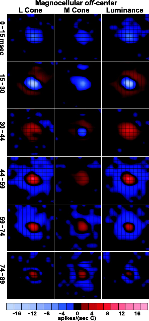
Spatiotemporal weighting functions of the same magnocellular neuron (Fig. 2) for multiple delays, from the 0 msec bin (0–15 msec) to the 74 msec bin (74–89 msec). Responses to different stimuli, shown fromleft to right: L cone, M cone, and luminance. Conventions are as in Figure 2. Off-center response starts in the 0 msec bin, peaks in the 15 msec bin, and reverses sign (rebounds) at either 30 or 44 msec. On-surround starts at 15, peaks at 30, and reverses at 44 msec. The M-cone response is delayed slightly relative to the L-cone response. Scale at bottomindicates response magnitudes in spikes/(sec · C), where C is the cone contrast of the stimulus.
First let us consider the luminance movie in the right-hand column of Figure 3. For the first delay that is illustrated, denoted 0–15 msec, there is a small but clear off (decrement excitatory) response. This means that this magnocellular cell had a receptive field center with a latency of response <15 msec (as did one other cell; these exceptionally fast cells were fairly peripheral, ∼20° from the fovea). The response of the center peaked in the range 15–30 msec and then changed sign from 30 up to 89 msec. The on (increment excitatory) surround is slower to respond than the center. The first significant surround on response occurs in the 15–30 msec time period. The surround also has a rebound but later, after 44 msec when the receptive field inverts its sign completely; compare the images at 15–30 and 44–59 msec.
The L-cone spatiotemporal weighting function has almost exactly the same time course as that of the luminance signal. The M-cone responses in the center begin just as rapidly as those of the L cone, at 0–15 msec, but M-cone rebounds, both center and surround, are delayed compared with those of the L cone. Such a qualitative difference between L- and M-cone dynamics may be attributable to the retinal contrast gain control (Shapley and Victor, 1981; Benardete et al., 1992). Because the L-cone stimulus was more effective in driving the cell than the M-cone stimulus, perhaps it also drove the contrast gain control mechanism more.
Magnocellular center and surround temporal weighting functions
A quantitative evaluation of the space–time maps can be made by inspecting the time evolution of center and surround components of the responses, plotted on the same scale (Fig.4). Responses of all pixels in the center and all pixels in the surround regions were summed separately to create temporal weighting functions (see Materials and Methods). In each panel of Figure 4 the temporal weighting functions for the center region (thick line) and for the surround region (thin line) are plotted as a function of time. Increment excitatory responses are positive in sign; decrement excitatory responses are negative. The temporal weighting functions for the magnocellular neuron (Fig. 4) are quite similar for L and M cones and for luminance modulation. The peaks of the center responses occur approximately one-half frame (∼7 msec) earlier than the surround peaks (interpolations not shown; see Materials and Methods). The M-cone response is ∼2–3 times smaller than the L-cone response both in center and surround.

Temporal weighting functions of the same magnocellular neuron (Figs. 2, 3) for receptive field center (thick lines) and surround (thin lines). Each data point is for a range of times between stimulus and response (sampled at the stimulus update rate, or 14.8 msec; short tick marks). The data points marked with caretscorrespond to responses during the first bin (in the range 0–14.8 msec). Time labels (long tick marks) are interpolated with respect to the data points (short tick marks), as specified in Materials and Methods. Note that the M-cone response is both weaker and somewhat slower than the L-cone response. All responses are in spikes/(sec · C), where C is the cone contrast of the stimulus.
Parvocellular spatial weighting functions
Parvocellular spatial weighting functions were measured in the same way as for magnocellular neurons, but the results were qualitatively different. Typical results from one L-on center and one M-off center neuron are shown in Figures5-7. The two neurons were recorded from the same penetration through the LGN: the off-center neuron from the contralateral eye, near the top of the LGN (presumably layer 6), and the on-center neuron from the ipsilateral eye, 1.85 mm further ventral (presumably layer 3).

Spatial weighting functions and radial weighing functions of two parvocellular neurons as measured with L-cone-isolating, M-cone-isolating, and luminance-modulated stimuli (conventions are as in Fig. 2). A, L-on/M-off neuron, 9° eccentric. The on-center/off-surround luminance response was used to define the receptive field center, outlined in white(see Materials and Methods). Note that neither the center cone type (L) nor the surround cone type (M) exhibits center/surround opponency (Fig. 1, arrow). B, M-off/L-on neuron, 11° eccentric. Although the signatures of the L-cone and M-cone responses are the same as in A, the M-off response dominates. Total region shown, 1.0° on a side; pixel size, 7.5 min. Delay between stimulus and response, 15–44 msec, the sum of the 15–30 and the 30–44 msec bins (see Materials and Methods). Because the luminance weighting function was much weaker than L-cone and M-cone weighting functions, it was multiplied by a factor of 2.0 to increase visibility. Conventions are as in Figure 2.
The sign of the dominant cone in parvocellular cells was judged from the luminance response. The luminance responses also were used to define the center regions (outlined in white; see Materials and Methods). For instance, the neuron that yielded the data in Figure5A was an on-center neuron as mapped with white light. The L-cone response was on in both center and surround, so we concluded that the L cone was the cone type that caused the on response of the center. The M-cone input to this neuron was off in both center and surround.
The examples shown are typical in that there were almost always 3–5 pixels in the centers of parvocellular neurons. For the most common pixel size (7.5 min) this corresponds to ∼1–2 times the typical diameter of receptive field centers, as measured in other studies at similar eccentricities and through the optics of the eye [for instance, Lee et al. (1998), ςc = 2–4 min; note that, for a difference-of-Gaussians model, the diameter of the center up to the zero crossing is ∼4–6 times the commonly quoted parameter for center size, its radius, ςc]. These sizes are large compared with the anatomical spreads of the dendrites of midget bipolar and midget ganglion cells that presumably constitute the retinal input to these neurons. They are also large compared with the local inhomogeneities of the cone mosaic measured recently in macaque and human retina (Roorda et al., 2001). Possible reasons for the comparatively large receptive field centers could be optical spread and/or neuronal coupling. That the macaque's physiological optics in large part determines the observed center sizes of parvocellular neurons is consistent with recent measurements ofMcMahon et al. (2000). They used laser interferometry to bypass the optics of the macaque's eye and observed higher spatial resolution of parvo-projecting ganglion cells than was measured through the natural optics. However, for the purposes of this paper the important issue is, can we resolve the center and surround through the natural optics? As evidenced in Figure 5, for example, the answer to that is affirmative.
The neuron for the data in Figure 5B was an off-center cell as mapped with white light; in this case the off input from the M cones dominated the response of the center. Note that both parvocellular neurons in Figure 5, A and B, received only on input from the L cones and off input from the M cones; they both were excited by red light and inhibited by green. The signature of the luminance response in the center, and also in the surround, was determined solely by the relative weight of the antagonistic L and M inputs.
It is remarkable that in these data we see no evidence for center/surround antagonism within a single cone type, although center/surround antagonism is observed in the luminance responses. This bears on the debate concerning mixed versus cone-specific surrounds (Wiesel and Hubel, 1966; Shapley and Perry, 1986; Lennie et al., 1991;Reid and Shapley, 1992; Lee et al., 1998). In Figure 1, it is shown that center/surround antagonism within a single cone type is the key test for distinguishing cone-specific versus mixed input to the receptive field surround. Let us consider for the neuron in Figure5A how center/surround antagonism arises in the luminance responses although there is none in its L- or M-cone-isolated responses. The biggest response from either L or M cones is concentrated in a small number of pixels (outlined in whitein the Fig. 5) in the center of the receptive field. The L-cone response is somewhat stronger in driving the center of this neuron, so when white light is used and drives the L and M cones equally, the L-cone on response predominates and the neuron is on-center. However, the L-cone spatial weighting function declines more steeply with position than does that of the M cone; thus the off response of the M cone predominates in the surround region when luminance stimuli are used. The data for the neuron in Figure 5B are similar except that for this neuron the stronger signals in the center came from the M cone, and the stronger signals in the surround came from the L cone. Data like those in Figure 5, A and B, suggest a high degree of specificity of cone functional connections to parvocellular neurons. They also confirm directly, for parvocellular neurons, the DOG model (Rodieck, 1965; Enroth-Cugell and Robson, 1966) of center/surround antagonism. In this model the center/surround receptive field is a result of the summation of two opposed spatial mechanisms that both have peak sensitivity in the center of the receptive field but that have different spatial spreads.
Parvocellular movies: spatiotemporal weighting functions
The nature of cone–cone interaction is such a central issue for understanding primate color vision that we studied it further by using dynamic measurements in parvocellular neurons. Representative response movies of parvocellular neurons are shown in Figure6, A and B, from the same neurons that yielded the data snapshots in Figure 5,A and B. Each row is from a given time offset as marked in the figure. As in the peak responses illustrated in Figure 5,A and B, the cone responses in these parvocellular neurons are of one sign at each particular time. For instance, in Figure 6A at both 15–30 msec and also from 30–44 msec, the L cone responses are all on, and the M cone responses are all off. The on-center/off-surround structure of the luminance response arises because L-cone excitation predominates in the center, whereas the M-cone input is slightly stronger in the surround. Later in time there is a zero crossing and change in sign of response (the rebound), as can be seen for both cells (Fig.6A,B). The peaks, zero crossings, and rebounds of the center responses lead those of the surround. It is worth noting that the zero crossings and rebounds occur later in time for parvocellular compared with magnocellular neurons; this probably reflects differences in retinal postreceptoral processing in the two parallel pathways.

Parvocellular center and surround temporal weighting functions
A second way to evaluate the degree of cone specificity in the parvocellular pathway is to examine the temporal weighting functions of the separate cone inputs to center and surround, as done earlier for the magnocellular neurons. The temporal weighting functions in Figure7 represent the dynamics of the responses of the parvocellular neurons from Figures 5 and 6. Each row is for a single neuron: the upper row is for the L-on/M-off neuron of Figures5A and 6A, whereas the lower row is for the M-off/L-on neuron of Figures 5B and6B. Note the opposite sign of cone-specific signals (L, positive; M, negative) in both the center (thick lines) and in the surround (thin lines). Also, the relative strength of center and surround cone-specific responses can be appreciated. It is most important that the center cone type (the L cone in Fig. 7A; the M cone in Fig. 7B) has a stronger response in the center and a weaker but same-sign response in the surround. The surround cone type (the M cone in Fig. 7A; the L cone in Fig. 7B) has peak sensitivity in the center but is relatively stronger in the surround and also does not change sign between center and surround. The antagonistic surrounds, which might appear noisy at any given pixel in the spatial or spatiotemporal plots (Figs. 5, 6), are quite robust in the temporal weighting functions in Figure 7, which are averaged over many pixels.

Temporal weighting functions of the same two parvocellular neurons (Figs. 5, 6). A, L-on/M-off neuron. Note that the L-cone response is on in both the center (thick line) and in the surround (thin line), but the center response is stronger. The M-cone response is off in both regions, but the surround is stronger. The opposite relationships between center and surround hold for the M-off/L-on neuron (B). Conventions are as in Figure 4.
Blue–yellow opponent receptive field
Four neurons in our sample responded robustly to an S-cone-isolating stimulus. Three of these were blue-on cells; they had S-on responses that were antagonized primarily by L-off responses, whereas responses to the M-cone stimulus were weak or negligible. In each of these cells the spatial extent of the L-off response was smaller than that of the S-on response. We nonetheless call these neurons S-on/L-off (rather than L-off/S-on) for consistency with the usual nomenclature: blue-on/yellow-off. In Figure 8, we show the spatial weighting functions of one such neuron, as measured with L-, M-, and S-cone stimuli, as well as a 100% contrast luminance stimulus.
The L-off response for this cell spans a region of ∼0.38° (3 pixels). The S-on responses are distributed over a considerably larger region, almost 1°. Consequently, the measured luminance responses appear off-center/on-surround. The receptive field structure attributable to the M cones is perhaps on-center (at only 1 pixel) but predominantly off in the surround, but the responses are much weaker than those attributable to the other two cone types. The large area of S-cone input was noted in studies of S-on cells in the retina (small bistratified cells) (Zrenner and Gouras, 1981; Dacey and Lee, 1994;Chichilnisky and Baylor, 1999), although most studies report that the antagonistic inputs from L and M cones are equal in size. Although we find differently, our small sample does not permit us to draw strong conclusions from this difference. Further, chromatic aberration in the optics of the eye could play a role in these measurements (Flitcroft, 1989). We focused the eyes to maximize the responses of red–green opponent parvocellular cells to achromatic gratings, so the stimuli that drive S cones may have been defocused.
The S-on neuron illustrated here (Figs.8, 9) was recorded 135 μm below the parvocellular neuron for which the responses are illustrated in Figures 5A–7A, which was in the second layer that was encountered driven by the ipsilateral eye. It was therefore probably near the bottom of parvocellular layer 3. Although histological analysis was not performed, this location is consistent with other work in which neurons with S-cone input were found in the middle two intercalated layers, located between the two ventral parvocellular layers (4 and 3) and between the parvocellular and magnocellular divisions (layers 3 and 2) (Hendry and Reid, 2000) (also see Schiller and Malpeli, 1978; Martin et al., 1997). A second S-on neuron was found 300 μm below this one.

Spatial weighting functions and radial weighing functions of an S-on/L-off neuron (12° eccentric, recorded at the bottom of the parvocellular layers), as measured with L-, M-, and S-cone-isolating and luminance-modulated stimuli. Total region shown, 1.25° on a side; pixel size, 7.5 min. Delay between stimulus and response, 15–44 msec, the sum of the 15–30 and the 30–44 msec bins (see Materials and Methods). The luminance weighting function was multiplied by 2.0 to increase visibility. Conventions are as in Figure2.

The spatiotemporal weighting functions for this S-on/L-off neuron illustrate a feature that was characteristic of the three blue-on cells we recorded. In both the magnocellular and the red–green opponent parvocellular neurons, the center mechanism is significantly faster than the surround. In the cells with S-on input the S-cone input spans a larger region (so we have called it the surround), but its time course is faster than the L-off input to the center. At delay of 15–30 msec the S-on response is robust, but the L-off response is barely out of the noise. Note that this initial phase of the S-cone response is as fast as the center responses in the red–green opponent parvocellular neurons (Fig. 6). The S-on response has a weak rebound (see Zrenner and Gouras, 1981) that begins at a delay of between 59 and 74 msec. By contrast, the L-cone rebound begins at 89 msec and is weaker yet. These differences in the dynamics of S-cone and L-cone inputs lead to the unusually prolonged off response of this neuron to a luminance stimulus. At short delays (30–59 msec) the luminance-off response is caused by the L-off response; at later delays (59–74 msec) it is caused by the rebound from the S-on response. These qualitative features of the dynamics of the blue-on cell are best appreciated in the temporal weighting functions (Fig.10E).

Temporal weighting functions for all red–green opponent parvocellular neurons (A–D) and S-cone-dominated neurons (E, F). For each cell type three or four sets of temporal weighting functions are plotted separately for both center (top) and surround (bottom); L-cone, M-cone, luminance, and, for some cells, S-cone responses are shown. For each cell all weighting functions are normalized by the same value. Red–green responses are normalized by the peak of the center response for the center cone type (L cone in A, B; M cone in C, D). S-on/L-off responses (E) are normalized by the S-cone surround peak (which was stronger than the S center). S-off responses (F) are normalized by the S-cone center. Data from four neurons that gave the weakest responses [normalization value <3.0 (spikes/sec)/(unit contrast)] are plotted in gray. Note that for red–green neurons the center cone types (L cone, A, B; M cone,C, D) have the same sign responses in the center and surround (with only two clear exceptions, shown byarrows). The luminance responses, however, have opposite signs in the center and surround.
Population studies: temporal weighting functions for receptive field center and surround
The spatial and temporal weighting functions for receptive field center and surround presented above are for typical examples of magnocellular and parvocellular neurons. We now present several figures that display quantitative features of the cone maps in the population of LGN cells that were studied. First we display the temporal weighting functions of center and surround, introduced in Figures 4 and 7. The temporal weighting functions illustrate the relative magnitudes of cone inputs and also their dynamics. Because of the controversy concerning the composition of the parvocellular surround, the temporal weighting functions of the four classes of red–green opponent neurons are presented first.
L-on/M-off cells
The temporal weighting functions of all nine L-on/M-off cells (Fig. 10A) were quite consistent; with only one exception, the cone-isolated responses had the same sign in center and surround. That is, L-cone responses were on everywhere and M-cone responses were off everywhere. For one cell of nine (Fig. 10A,arrow) the L-cone response changed sign in the surround and so showed a pronounced off response. This is one of only two examples we found of spatial antagonism for a cone-isolated response: the hallmark of a mixed surround. For all other cells the magnitudes of the L-cone responses in the center were stronger than in the surrounds, but the M-cone responses were similar in both center and surround. This resulted in the dominance of the L-on responses in the center and the M-off responses in the surround.
L-off/M-on
The temporal weighting functions of the eight L-off/M-on neurons (Fig. 10B) were also quite consistent, again with only one outlier. As a rule, cone-isolated responses had the same sign throughout the receptive field, and L-cone signals were opposite in sign to M. In the center the L-off responses were stronger than the M-on. In the surround the M-on response was stronger than the L-off. The only exception (marked with an arrow, Fig.10B) showed spatially antagonistic input from the L cone. This cell was encountered in the same penetration as the exceptional, mixed surround cell in the L-on/M-off group (above), but in a different parvocellular lamina 1.3 mm ventral.
For the other seven L-off/M-on neurons (Fig. 10B) the dynamics of the L-off responses should be noted. Although the initial response was L-off in the surround (Fig. 10B,bottom), this L-off response was less sustained than in the center (Fig. 10B, top). This effect is hard to discern when the responses of all cells are superimposed on separate plots of center and surround (as in Fig.10B), but it is quite evident when center and surround for each cell are plotted on a single axis (as seen in Fig. 7; analysis not shown). It is possible that this relative transience could have been attributable to an L-off center partially superimposed with a weak L-on surround in many of these cells, which would mean they had a mixed surround. To test this possibility, we examined the temporal weighting functions of annuli, starting at different distances from the center. At no distance from the center were the transient L-off responses converted to L-on responses. In other words, at no distance from the center were responses elicited from the L cones that were opposite in sign to the L-off responses in the center. Therefore, the hypothesis of a mixed surround was not supported by these data.
M-on/L-off and M-off/L-on
The temporal weighting functions of all 10 M-cone-dominated cells (Fig. 10C,D) showed no positive evidence of a mixed surround. Specifically, center/surround opponency was not seen in their M-cone responses. Of the four classes of red–green opponent neurons, M-on/L-off cells (Fig. 10C) received the most balanced input from the L and M cones to the center. The luminance responses (with one exception) were therefore weak. In three cases an antagonistic surround could not be demonstrated in the luminance responses (Fig. 10C, bottom right); therefore, strong arguments cannot be made for the cone composition of the surround in these cells (if indeed there was one; see Fig.15D). In the M-off/L-on cells (Fig. 10D), however, overt spatial opponency was seen clearly in the luminance responses, but never in the M-cone responses.
S-on and S-off
The temporal weighting functions of the three cells that received S-on input (Fig. 10E) were all quite similar. As noted for Figure9, the responses of the S-on neurons had particularly weak rebounds. Further, as was the case for the cell illustrated in Figures 8 and 9, the region of S input was always larger than the region of antagonistic off input, which was dominated by the L cone. Their receptive fields as mapped with luminance stimuli (far right column here and in Figs. 8, 9) therefore all appeared off-center/on-surround. The only cell we found that received S-off input (Fig.10F) was quite different in character. The responses were quite weak, on the order of 2 (spikes/sec)/(unit contrast), and were dominated almost entirely by the S cone, both in the center and in the nonantagonistic surround.
Magnocellular
Finally, the temporal weighting functions for the on-center (Fig.11A) and off-center magnocellular neurons (Fig. 11B) were very consistent within each class but quite different from those of parvocellular neurons. In the centers the M and L-cone responses were both of the same sign (although the L-cone responses were stronger); in other words, there was no red–green opponency. In most cases, however, the single-cone inputs (both L and M) as well as the luminance responses were spatially opponent. Contrary to what we found for parvocellular neurons, single-cone maps were usually center/surround antagonistic. The exceptions were three on-center cells that were predominantly M-on in both the center and surround. Because the surrounds of these cells were also L-off, the surrounds were color-opponent (see Figs.14B, 16B).

Temporal weighting functions for all magnocellular neurons. For each cell type three or four sets of temporal weighting functions are plotted separately for both center (top) and surround (bottom); L-cone, M-cone, luminance, and, for some cells, S-cone responses are shown. For each cell all weighting functions are normalized by the same value, the peak of the luminance response.
Sustained and transient dynamics
The dynamics of the parvocellular temporal weighting functions in Figure 10 are interesting because they differ from magnocellular temporal weighting functions in having a smaller rebound compared with the peak response. This is important because the relative strength of the rebound is related directly to the transience of the response to a step stimulus (Gielen et al., 1982; Usrey et al., 1999; De Valois et al., 2000; Usrey and Reid, 2000). The integral of a temporal weighting function should be approximately equal to the sustained component of the step response. For magnocellular neurons the integrals of the temporal weighting functions are near zero, but for parvocellular neurons they are not. By comparing the data for parvocellular and magnocellular neurons in Figures 10 and 11, one observes that the different dynamics are present in the cone-isolated responses as well as in the responses to achromatic stimuli. To make this observation more quantitative, we devised a measure of sustained-ness intended to approximate the sustained firing rate of the step response divided by its peak firing rate. The sustained component is the ratio of the area under the temporal weighting function integrated over its entire duration (0–222 msec, or 15 stimulus frames) divided by the area under the waveform up to the first zero crossing. For temporal weighting functions that are monophasic with no undershoot, the sustained component is 1. For temporal weighting functions that are biphasic and for which the rebound exactly cancels the initial peak, the sustained component is 0. Figure12A is a histogram of the distribution of the sustained component across our population of macaque LGN units in response to luminance m-sequences, and it is consistent with the well known distinction between parvocellular and magnocellular neurons as sustained and transient, respectively (Dreher et al., 1976; De Valois et al., 2000). The distribution falls into three distinct clusters: magnocellular neurons with sustained component near 0, red–green opponent parvocellular neurons with sustained component near 0.5–0.6, and S-cone-driven neurons (although few in number) with sustained component near 0.9 (see Zrenner and Gouras, 1981). Figure 12B displays the novel result that the same tripartite distribution of sustained-ness is observed in responses to cone-isolating m-sequences for the dominant cone type (L cone for magnocellular; the center cone type, L or M, for red–green opponent parvocellular; and the S cone for blue-on cells). This implies that the degree of sustained-ness or transient-ness is not caused by subtraction of the signals of the cones in response to achromatic patterns but, rather, must be a result of different temporal filtering in the retinal circuitry that drives the parvocellular and magnocellular neurons in parallel.

Histogram of the sustained component (see Results) of all magnocellular neurons, red–green opponent parvocellular neurons, and blue-on cells. A, Responses to luminance stimuli. B, Responses to cone-isolating stimuli for the dominant cone type (L cone for magnocellular, center cone for red–green parvocellular, S cone for blue-on). The three populations were nonoverlapping, whatever the stimulus type.
Relative weights of cone mechanisms in the center and surround across the population of LGN cells
To compare the amplitude of the single-cone responses across the population of LGN cells, we compressed the temporal weighting functions of center and surround to a single number: the strength of response attributable to each of the cone classes (or to the achromatic stimuli). These strengths were calculated by integrating the initial portions of the temporal weighting functions up to the first zero crossing that followed the peak. Because surround responses were generally slower than center responses, integrating the center and surround separately provides a more valid measurement of their relative strength than would be obtained by considering static spatial weighting functions (as seen in Fig. 5). Six different cone strengths were determined: the strengths of L, M, and S both for the center (cl
, cm
,cs
) and for the surround (sl
, sm
,ss
). Also, the data allowed us to calculate the total strength of the achromatic (luminance) responses to center and surround, ca
and sa
. Finally, we defined the total strength t as the sum of the center and surround strengths, for instance:

To compare the relative contribution of the three cone classes on a single plot, we normalized each response strength by the sum of the absolute values of all three, following Derrington et al. (1984). We refer to these normalized cone strengths as cone weights. For instance, the L-cone weight to the center is given by:
 By definition, the sum of the absolute values of the weights ( Cl
, Cm
, andCs
) is 1.0. If two of the three are plotted against each other, the absolute value of the third can be inferred. As in Derrington et al. (1984), Cm
has been plotted versus Cl
in Figure13. The distance from each point to the diagonal borders of the figure gives the absolute value of the S-cone weight (points outside the borders indicate cells for which no S-cone measurements were made).
By definition, the sum of the absolute values of the weights ( Cl
, Cm
, andCs
) is 1.0. If two of the three are plotted against each other, the absolute value of the third can be inferred. As in Derrington et al. (1984), Cm
has been plotted versus Cl
in Figure13. The distance from each point to the diagonal borders of the figure gives the absolute value of the S-cone weight (points outside the borders indicate cells for which no S-cone measurements were made).

Scatter plots of normalized cone weights, following Derrington et al. (1984), plotted for all neurons recorded in parvocellular layers. Shown are M-cone weights plotted versus L-cone weights, in which magnitudes of S-cone weights are determined by the distance from diagonal lines. Points near the diagonal lines are from cells that received negligible S-cone input. Points for which no S-cone measurements were performed are plotted outside the diagonal lines. Symbols signify the eight classes of cells. Antagonistic L-cone versus M-cone responses are in the second (II) and fourth (IV) quadrants. Nonantagonistic (mixed) responses are in the first (I) and third (III) quadrants. Each class clusters distinctly in the plot ofCenter weights (A), but less so in plots of Surround (B) andTotal (C) weights. The two cells that had clear mixed surrounds (Fig. 10A,B) are indicated with arrows (B).
Note that the cone weights of the centers of the four types of red–green opponent parvocellular neurons clearly are clustered (Fig.13A). The neurons excited by green (M-on/L-off and L-off/M-on) are found on the border in the second quadrant. The tick mark on this border indicates the position at which the L and M cone weights are equal and opposite: Cm = 0.5;Cl = −0.5. Points for the M-on/L-off neurons cluster above the tick mark; those for the L-off/M-on neurons cluster below the tick mark. Neurons that were excited by red (L-on/M-off and M-off/L-on) cluster on the border in the fourth quadrant. Again, the tick mark segregates the on-center from the off-center neurons. Finally, points for the three S-on neurons all fall near thex-axis. This indicates that the M-cone input to the antagonistic mechanism was quite weak.
The plot of cone weights for the receptive field surrounds (Fig.13B) addresses the question of whether the surround is cone-specific or mixed. Most points for the red–green parvocellular neurons (circles and squares; see legend) fall in the second and fourth (cone-opponent) quadrants. This is evidence in favor of a cone-specific surround, because if the surround were mixed, one would expect the cone weights of the surround to be the same sign (first and third quadrants). The only two clear exceptions are marked with arrows, as they are in Figure 10, A and B. Three other points for L-center cells fall in the “nonopponent” first and third quadrants of Figure 13B, but near they-axis, where the L-cone weight is almost zero. We think that these data points are not positive evidence for the mixed surround hypothesis, however, because they correspond to cases in which the L-cone surround responses were simply weak and noisy (see Fig.15A, specifically the three points near thex-axis).
Figure 13C shows the plot of M-cone versus L-cone weights integrated over the entire receptive field. It represents the predicted cone weights that would be obtained with stimuli larger than the receptive field. This is equivalent to the similar plot in Derrington et al. [(1984), their Fig. 6] and shows a similar result: red–green opponent neurons cluster in the second and fourth quadrants with approximately equal and opposite weights.
Plots of the L and M cone weights for the magnocellular neurons in our sample (Fig. 14) demonstrate that the receptive field center receives mixed, synergistic L- and M-cone input (Fig. 14A), as does the surround in most cases (Fig.14B). In three cases, however, the surround in fact received antagonistic L- and M-cone input (Fig. 14B), as indicated by points in the second quadrant. These exceptions, all on-center neurons [perhaps the type IV cells of Wiesel and Hubel (1966)], in fact received antagonistic L-off and M-on inputs in the surround. Weakly opponent cone weights (points in the second and fourth quadrants near one of the axes) were yet more common for the total responses (the sum of the center and surround; Fig. 14C). These results are consistent with the findings of Smith et al. (1992)(see also Schiller and Colby, 1983; Derrington et al., 1984; Lee et al., 1989), who demonstrated cone-opponent responses in the surrounds of magnocellular cells.

Scatter plots of normalized cone weights for magnocellular neurons, as in Figure 13. On-center cells are indicated by symbols with light centers; off-center cells are indicated by symbols with dark centers.
Strengths of cone inputs to center and surround across the population
Because center and surround are considered separately in the cone weight plots, Figures 13 and 14, it is impossible to compare them for any given cell. Furthermore, all magnitudes in Figures 13 and 14 are relative, so response strengths cannot be appreciated. Therefore, in Figure 15 we plot the strengths of the surround versus the center responses for the entire population of parvocellular neurons that we studied. In this figure, points in the second and fourth quadrants indicate opponent center/surround interactions: on-center/off-surround in the fourth quadrant; off-center/on-surround in the second quadrant. Points plotted in the first and third quadrants indicate that the center and surround had the same sign of response. These plots illustrate that red–green parvocellular neurons generally had spatially opponent receptive fields when mapped with luminance stimuli (Fig. 15D), but the centers and surrounds had the same sign of response when the cells were driven with L-cone- and M-cone-isolating stimuli (Fig.15A,B, with two exceptions shown by arrows).

Scatter plots of response strengths (not normalized) in the surrounds versus the centers for L-cone (A), M-cone (B), S-cone (C), and luminance responses (D) in units of spikes/(sec ·C), where C is the cone contrast of the stimulus. Data are shown for all neurons recorded in parvocellular layers; the symbols are as in Figure 13. Antagonistic center/surround responses fall in the second and fourth quadrants; nonantagonistic responses fall in the first and third quadrants (seeinsets). With few exceptions, all luminance responses (D) had antagonistic centers and surrounds. Most L-cone responses (A) and all M-cone responses (B) had nonantagonistic centers and surrounds (exceptions are indicated with arrows in A, as in Figs. 10, 13).
In a past report with an overlapping data set, we reported that more than one-third of parvocellular neurons were spatially nonopponent (type II cells) when measured with luminance stimuli (Reid and Shapley, 1992); here we instead found center/surround opponency (type I cells) in 23 of 27 cases (Fig. 15D). The difference is that here we considered independently the temporal weighting functions of center and surround in determining cone strengths rather than the responses at one time point, as in our previous report. Because of the relative delay between center and surround, we believe the present data analysis is more appropriate because it does not truncate the surround responses. When analyzed in this manner, all but one of the L-cone center cells had opponent centers and surrounds (Fig. 15D,circles), as did all five M-off cells (Fig. 15D,red squares). This can be seen more directly from the temporal weighting functions for luminance (compare top andbottom right of Fig. 10A,B,D). For three of five M-on cells, however, we did not measure an antagonistic surround with the luminance stimulus (Figs. 10D,15D, green squares).
Similar plots of response strengths for surrounds versus centers for magnocellular neurons illustrate the center/surround antagonism (Fig.16, points in the second and fourth quadrants), seen with both luminance (Fig. 16C) and cone-isolating stimuli (Fig. 16A,B). The only exceptions are for the three cells, noted above, that had on responses to M-cone stimulation in both the center and surround (Fig.16B, points in the first quadrant).

Scatter plots of magnocellular response strengths in the surrounds versus the centers for L-cone (A), M-cone (B), and luminance responses (C) in units of spikes/(sec · C), where C is the cone contrast of the stimulus. All luminance responses had antagonistic centers and surrounds, as did the L-cone responses. Three of the on-center cells did not receive antagonistic input from the M-cones in the surrounds (B, first quadrant), whereas three did (B, fourth quadrant).
Time courses of temporal weighting functions
So far, our analyses of the temporal weighting functions of the LGN population have focused on their magnitude. The time courses of these responses, however, were far from uniform; they differed between center and surround and between the different cone-isolating stimuli. These differences are appreciated readily from the raw temporal weighting functions (Figs. 4, 7, 10, 11). To be able to examine these differences across the population of LGN neurons, we determined the time of the peak response in each temporal weighting function.
First we compared the responses of the antagonistic L-cone and M-cone inputs in red–green opponent parvocellular neurons by plotting the peak time of the M-cone responses versus L-cone responses for the center pixels (Fig. 17A). With only one exception, the points for neurons with L-cone centers (circles) fell above or on the line of unit slope. All points for neurons with M-cone centers (squares) fell below the line of unit slope. This means that the time-to-peak was faster for the center cone type than for the antagonistic cone type (Gielen et al., 1982; Yeh et al., 1995). Although the effect was very consistent, in most cases the time difference between the peak response of L and M cones was small (Fig. 17C; L-center neurons, mean Δt = 2.6 msec; M-center neurons, mean Δt = −3.4 msec). Because the center cone type (whether it was M or L) was almost always faster, this result is consistent with the idea that L and M cones themselves have very similar dynamics and that what differences we observed were postreceptoral.

Peak times of L- and M-cone responses in centers (A–C) and of luminance responses in centers and surrounds (D–F). A, Scatter plot of M-cone peak times versus L-cone peak times for red–green opponent parvocellular neurons. L-cone responses were faster for L-cone center cells (circles), and M-cone responses were faster for M-cone center cells (squares); thesymbols are as in Figures 13-16.B, For magnocellular neurons the L-cone responses were faster. C, Histogram of differences between M-cone and L-cone peaks. D, E, Scatter plots of surround versus center peaks for red–green opponent parvocellular (D) and magnocellular (E) neurons. Three M-cone center cells with noisy surround responses had nominal peaks >60 msec. These cells were excluded. F, Histogram of differences between surround and center peaks. With two exceptions, all surrounds were slower.
For magnocellular neurons the L-cone responses were consistently faster than the M-cone responses (Fig. 17B), although the contrast of the L-cone stimulus (21%) was slightly lower than the contrast of the M-cone stimulus (24%). This may be related to the fact that the L-cone input was in most cases stronger than that of the M cones (Figs. 4, 11, 14). Again, the timing difference between L- and M-cone responses was fairly small (Fig. 17C; mean Δt = 3.9 msec).
Finally, we measured the time-to-peak of the responses of centers and surrounds as mapped with a luminance stimulus. The latencies to luminance stimulation of the center can be compared with other values in the literature. The times-to-peak of the magnocellular centers (Fig.17E, 20–37 msec; median, 24 msec) were comparable with latencies found in one recent study (Maunsell et al., 1999) in which step stimuli were used (median, 21 or 25 msec in two animals; the latency to half-maximal step response, a measure comparable with the peak of the impulse response measured here, was ∼3 msec later). Our measurements of magnocellular time-to-peak, however, were slightly faster than latencies found in another recent study of magnocellular step responses (step latency, 30 msec; Schmolesky et al., 1998) and, surprisingly, much faster than the times-to-peak found in a study that used techniques similar to our own (median, ∼60 msec; De Valois et al., 2000). For parvocellular neurons the times-to-peak we found (Fig.17D, 23–40 msec, median, 29 msec) were again similar to the latencies found in one recent study of step responses (median, 31 or 38 msec; Maunsell et al., 1999), but not another (median, 50 msec;Schmolesky et al., 1998). Again, they were much faster than the times-to-peak of the impulse responses measured by De Valois et al. (2000) for parvocellular neurons (median, ∼80 msec).
The luminance responses of the surrounds were significantly slower than those of the centers, both for parvocellular neurons (Fig.17D) (see Derrington and Lennie, 1984; Golomb et al., 1994;Benardete and Kaplan, 1997) and magnocellular neurons (Fig.17E) (see Derrington and Lennie, 1984). Although there was a broad range, on average the differences in peak times between surround and center were greater than the differences between L-cone inputs and M-cone inputs (Fig. 17F, note expanded scale; parvocellular mean, Δt = 9.5 msec; magnocellular mean, Δt = 8.3 msec).
It is important to emphasize the difference between the two timing comparisons we have made for parvocellular cells: between center and surround cone type (for cone-isolating stimuli; Fig. 17A,C) and between center and surround regions (for luminance stimuli; Fig.17D,F). The comparison between cone types is not a spatial one, because we have compared responses at the same pixels. The slight differences we found (center cone type faster than surround cone type) indicate differences in postreceptoral processing. The much greater differences between the luminance responses in center versus surround result primarily from the fast responses in the center (median, 29 msec), which are considerably faster than the responses to the center-type cone-isolating stimulus (median, 36 msec). The fast luminance response in the center comes about because it is the difference of two signals: a strong input from the center cone type minus a weaker, slightly delayed input from the surround. The surround response to luminance, however, is in large part the result of a single mechanism; to first approximation it peaks at the same time as the cone-isolated response of the surround cone type (luminance response in surround: median, 39 msec; surround-type cone-isolating stimulus in surround: median, 39 msec).
DISCUSSION
Cone inputs to parvocellular neurons
Two competing theories of red–green parvocellular neurons can be called the mixed surround and the cone-specific surround hypotheses. In both, the center mechanism is fed by a single cone class and is opposed by a larger surround mechanism. In both, the surround gets input from the other (noncenter) cone class that is opposite in sign to the input from the cone that drives the center. The crucial difference is that, in the mixed surround hypothesis, the cone type that drives the center also provides antagonistic input to the surround (Fig. 1), but in the cone-specific hypothesis the signals from the center cone do not change sign in the surround. Our experimental data are mainly consistent with the cone-specific hypothesis.
One can ask, what observable differences could decide between the two models? Most importantly, an analysis of the question must use independent criteria to differentiate the center from the surround so that the cone inputs to these two mechanisms can be characterized. These independent criteria can be either spatial or temporal. Although the center and surround have slightly different temporal response dynamics (Fig. 17), these differences alone have proven insufficient to differentiate between the mixed and cone-specific surround hypotheses (Lankheet et al., 1998). Our approach was a hybrid: we used spatial information to define the center and surround regions, and we used temporal information to quantify the responses within these regions (see discussion in Results of Figs. 10, 15D). We thereby demonstrated antagonistic center/surround responses to luminance stimuli in most parvocellular neurons (type I cells: 16 of 17 L-cone center; 7 of 10 M-cone center; cf. Reid and Shapley, 1992) but nonopponent responses to cone-isolating stimuli in all but two cases.
Other approaches to the spatial differentiation of center and surround are possible. Analysis of receptive fields with gratings at a range of spatial frequencies can provide measurements of small (center) and large (surround) mechanisms. Similarly, a bipartite field can be used to drive the surround strongly but also, by moving it across the receptive field, to measure the size of the center mechanism. It is striking that, when cone isolation is used with all three methods, m-sequence grids (this study), spatial frequency tuning (Shapley et al., 1991; our unpublished results), and a bipartite field (Lee et al., 1998), the same result has been found. The measured surrounds are not mixed but instead are cone-specific. A recent report (Martin et al., 2001) also is consistent with the conclusion of cone specificity in parvocellular neurons.
Despite this consistent finding obtained with multiple approaches, it is impossible to prove that the surround receives input from one cone type only. Optical blur could cause signals from the center to mask some mixing in the surround. As argued by Lee et al. (1998), however, the surround is likely to be at least biased. Specifically, they showed that their data (particularly for L-cone center cells) were mainly inconsistent with the extreme version of the mixed surround model: that cone inputs are entirely random.
No anatomical substrate has been found for specificity in the connections that cones make with horizontal cells in the primate retina (Boycott et al., 1987; Boycott and Wässle, 1999). There is also no evidence for cone specificity in the visual responses of primate horizontal cells (Dacheux and Raviola, 1990; Dacey et al., 1996, 2000). Furthermore, from inferences based on purely anatomical evidence,Calkins and Sterling (1999) conclude that there is no known retinal pathway for the cone-specific signals that are suggested by the physiology. Nevertheless, as discussed above, in the central 15° of vision the physiological evidence indicates only cone-specific input to receptive field surrounds of parvocellular neurons and their retinal inputs. However, in the far periphery of the retina, mixed cone input has been reported for both center and surround (Dacey, 1999). It is interesting to note that there is no known anatomical substrate for the color-opponent surrounds described in some magnocellular neurons and their retinal inputs (Figs. 14B,16B) (Wiesel and Hubel, 1966; Schiller and Colby, 1983; Derrington et al., 1984; Lee et al., 1989; Smith et al., 1992). Nevertheless, this physiological evidence for cone specificity has met with little controversy.
Another important question is, what do our results indicate about the functional role of parvocellular neurons? The near universal presence of cone-specific overlapping antagonistic mechanisms in parvocellular neurons means that these cells are committed to being sensitive to color at the expense of achromatic sensitivity. Indeed, for many red–green parvocellular neurons, the L and M opponent inputs overlap in space to a great degree and tend to cancel each other out when presented with an achromatic stimulus. For very fine achromatic spatial patterns the center cone may become dominant, but for the typical range of spatial frequencies in natural scenes, the red–green parvocellular neurons are designed to take the difference between L and M cones. One consequence of cone specificity is that sensitivity to color contrast is greater than if the surround were mixed, especially for stimuli that are large or low spatial frequency. The finding of cone specificity of the surround is consistent with the concept that maximizing color contrast sensitivity for large area stimuli is one of the major functional goals of parvocellular neurons.
Cone inputs to magnocellular neurons
Magnocellular neurons have strikingly different cone inputs from those seen in parvocellular neurons. For instance, these neurons most often exhibit a center/surround organization of their cone-isolated responses as seen in Figures 2 and 3 for both L and M cones. Such a pattern almost never is observed in parvocellular neurons. There is evidence for cone specificity in some magnocellular surrounds, because some receive antagonistic M–L cone input. However, the magnocellular center mechanisms are very much the same from one cell to another in receiving additive input from L and M cones, with a preponderance of input from L cones.
One can ask, what do the spatiotemporal cone maps tell us about the visual function of magnocellular neurons? Magnocellular neurons have much higher achromatic contrast sensitivity than parvocellular neurons (Shapley et al., 1981; Kaplan and Shapley, 1982, 1986; Hicks et al., 1983; Blakemore and Vital-Durand, 1986; Spear et al., 1994). The cone maps and cone weights provide an explanation for such a difference. Achromatic stimuli drive all the cones simultaneously so the responses of cones to these stimuli are in-phase. For red–green parvocellular neurons that subtract M and L cone signals, these in-phase modulations tend to cancel out, producing poor sensitivity. For magnocellular neurons the synergy of the cone signals in this case causes responses to achromatic stimuli to be large. For purely chromatic modulation between red and green the L and M cone modulations are out of phase, so the situation is reversed compared with the achromatic case. For red–green modulation the L and M cone signals tend to cancel in magnocellular neurons. Thus magnocellular neurons are “blind” to color modulation, especially for fine patterns, small spots, or narrow bars that excite only the center mechanism of the magnocellular neurons. Our results confirm others (such as Smith et al., 1992) in that magnocellular neurons can have surrounds that are color-opponent. This means that for very coarse patterns or large stimuli the magnocellular neurons will respond to color modulation. At present, there is no known function of this low spatial resolution color response in magnocellular neurons.
Dynamics of center versus surround and L- versus M-cone inputs
Our measurements allowed us to compare the time course of responses both between center and surround and also between the different cone classes. For magnocellular and red–green opponent parvocellular neurons we found differences of both sorts: a large relative delay between center and surround (for achromatic stimuli) and smaller delays between L- and M-cone contributions to the center.
The dynamics of responses of center and surround to achromatic stimuli were markedly different in both parvocellular and magnocellular neurons (Figs. 10, 11, 17D–F) (Derrington and Lennie, 1984;Benardete and Kaplan, 1997). These differences are likely to derive in large part from retinal mechanisms, because they also are found in recordings of synaptic (S) potentials in the LGN (our unpublished observations). The time-to-peak of the center response was typically 8–10 msec earlier than that of the surround. This result indicates that neural signals traveling to the neuron from the surround suffer more delay or more temporal averaging; hence their response peaks later. This difference between center and surround dynamics could cause temporal modulation to have significant effects on color perception (Courtney and Buchsbaum, 1991).
In parvocellular cells the responses of the center cone type were faster than those of the surround cone type (Fig. 17A,C), as had been found in studies that used full-field cone-isolating stimuli (Gielen et al., 1982; Yeh et al., 1995). In magnocellular neurons we found that the responses of the L cones in the receptive field center were faster than the responses of the M cones (Fig.11A,B); specifically, their responses typically peaked ∼4 msec earlier (Fig. 17B,C). This is probably postreceptoral, because there was no such consistent asymmetry between L and M cones for parvocellular neurons (Fig. 17A,C). One would expect this time delay to have an effect on the equiluminant point measured with fast flickering stimuli; the red–green balance at equiluminance should require more green, shifting toward the null point of the L cones as the flicker rate increases. In humans it has been shown that, for the identification of a moving stimulus, the L cone dominates at higher temporal frequencies (Gegenfurtner and Hawken, 1995); this psychophysical effect could be caused by the different cone dynamics in magnocellular neurons.
Footnotes
This work was supported by National Institutes of Health Grants EY1472 and EY12185 and by a grant from the Sloan Foundation. We thank Jonathan D. Victor for help with generating the visual stimuli and W. Martin Usrey, Michael J. Hawken, and John Pezaris for critical readings of this manuscript.
Correspondence should be addressed to Dr. R. Clay Reid, Harvard Medical School, Department of Neurobiology, Goldenson, Room 203, 220 Longwood Avenue, Boston, MA 02115. E-mail: clay_reid{at}hms.harvard.edu.


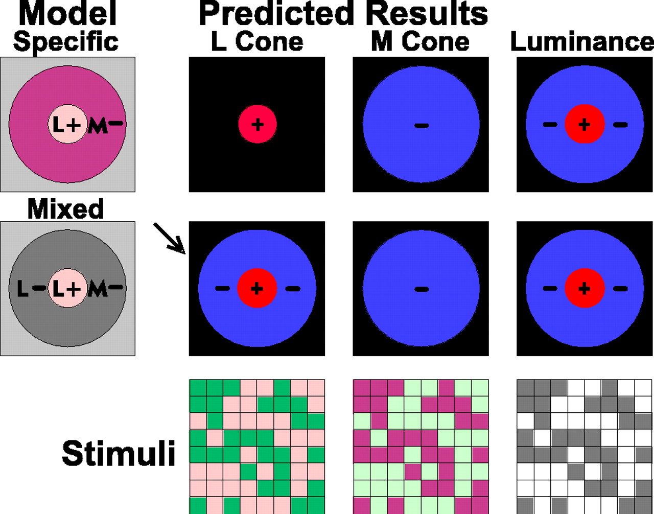