

Abstract
Spatial perception, the localization of stimuli in space, can rely on visual reference stimuli or on egocentric factors such as a stimulus position relative to eye gaze. In total darkness, only an egocentric reference frame provides sufficient information. When stimuli are briefly flashed around saccades, the localization error reveals potential mechanisms of updating such reference frames as described in several theories and computational models. Recent novel experimental evidence, however, showed that the maximum amount of mislocalization does not scale linearly with saccade amplitude but rather stays below 13° even for long saccades, which is different from predicted by present models. We propose a new model of perisaccadic mislocalization in complete darkness to account for this observation. According to this model, mislocalization arises not on the motor side by comparing a retinal position signal with an extraretinal eye position related signal but by updating stimulus position in visual areas through a combination of proprioceptive eye position and corollary discharge. Simulations with realistic input signals and temporal dynamics show that both signals together are used for spatial updating and in turn bring about perisaccadic mislocalization.
Introduction
Our eyes move to sample the environment with high resolution at the center of gaze. This advantage comes with the cost of a fragmented visual input stream leading to the problem of maintaining visual stability (Wurtz, 2008). While visual input changes with each eye movement, our experience of the visual world is rather stable and not centered on the individual views. One line of research to study visual stability has focused on the localization of perisaccadically flashed stimuli in total darkness. It has been observed that, even before saccade onset, briefly flashed stimuli are mislocalized in saccade direction. The magnitude of misperception depends mainly on the interval between saccade onset and stimulus flash, regardless of stimulus position (Matin et al., 1970; Honda, 1989, 1991; Dassonville et al., 1992; Schlag and Schlag-Rey, 2002). Different models have been developed using the concept of a continuous eye position signal. Dassonville et al. (1992) suggested that, since misperceptions already occur presaccadically, the eye position information is sluggish and anticipates the saccade. Pola (2004) proposed a more elaborate model accounting for delay and visual persistence and concluded that the extraretinal signal may only change after saccade onset. Similarly, imposing the additional constraint of no mislocalization for continuously visible stimuli, Teichert et al. (2010) proposed that reafferent position information is sufficient to explain perisaccadic shift.
However, the mapping of these rather abstract models onto brain structures and mechanisms is still unidentified (Hamker et al., 2011). Moreover, an electrophysiological correlate of a psychophysical, continuous eye position signal is still lacking, although eye position-dependent responses are known to exist in different brain areas, as the parietal cortex (Andersen et al., 1990; Galletti et al., 1993; Bremmer et al., 1997). A correlate of eye position has been identified in monkey somatosensory cortex (Wang et al., 2007). However, this signal neither anticipates the eye movement nor does it shift continuously but rather jumps from the previous to the new fixation. A corollary discharge, here a copy of a motor command from the superior colliculus, can provide anticipatory information about upcoming eye movements (Sommer and Wurtz, 2004). However, since it encodes the saccade displacement, it does not hold as a continuous eye position signal.
In addition to the anatomical and physiological uncertainties, a problem of present models of perisaccadic localization in total darkness was recently discovered by Van Wetter and Van Opstal (2008). They found that the maximum amount of mislocalization saturates around 12° even for long saccades up to 35°, whereas current models predict that mislocalization scales linearly with saccade amplitude (Van Wetter and Van Opstal, 2008).
Based on electrophysiological observations of corollary discharge (for review, see Sommer and Wurtz, 2008) and eye position in primary somatosensory cortex, we developed a novel model of perisaccadic perception in total darkness using a combination of eye position and corollary discharge. It explains the error in localization, the saturation of its magnitude, and a reduction of its magnitude with increased stimulus duration from the temporal dynamics in the model as the eye-related signals change around saccade.
Materials and Methods
Our model for perisaccadic localization (Fig. 1A) is assumed to be located in the lateral intraparietal area (LIP). LIP is known to have neurons with retinocentric receptive fields that are modulated by eye position (Andersen et al., 1990; Bremmer et al., 1997) and saccade plans (Colby et al., 1996; Kusunoki and Goldberg, 2003), which makes it a likely area for the computations described in our proposed model. In this model, we simulate two different kinds of neurons in LIP. Both neuron types have retinocentric receptive fields. However, one type of neurons is gain modulated by a proprioceptive (PC) eye position signal, which encodes the eye position in the orbit but does not update simultaneously with the eyes during saccades. The eye position signal of these neurons updates after saccade, similar to the updating of gain fields in LIP (Xu et al., 2010). Such a proprioceptive eye position signal could arise in somatosensory cortex (Wang et al., 2007), or alternatively, in the central thalamus (Tanaka, 2007). The other neurons in the model LIP are gain modulated by a corollary discharge (CD), which is assumed to originate in the superior colliculus (SC) (Sommer and Wurtz, 2004, 2008). It encodes eye displacement (i.e., retinotopic position of the saccade target) and is active around saccade onset. The CD is probably routed via the frontal eye field (FEF) where it is subject to an eye position gain field (Cassanello and Ferrera, 2007), which we assume to be also driven by the proprioceptive signal. This implicit eye position information in the CD signal is required to allow a combination of eye in the orbit with eye displacement information by lateral interactions as will be explained in more detail later. The activity of all simulated LIP neurons is decoded to determine the response of the model (i.e., the perceived spatial position) by a multiple-option diffusion model with decision neurons to obtain a spatial percept (Usher and McClelland, 2001; Hamker, 2007). As justified by empirical studies (Kiani et al., 2008; Stanford et al., 2010), this approach has the important advantage of accumulating varying evidence over time compared with time averages or snapshots. However, we do not necessarily assume that such decoding takes place in parietal cortex. Due to the anticipatory CD, some of the simulated LIP cells are modulated already presaccadically consistent with previous observations (Duhamel et al., 1992; Colby et al., 1996; Kusunoki and Goldberg, 2003).

A, Our model of perisaccadic shift is composed of two cell types (in LIP), XbPC and XbCD, which receive retinal input from early extrastriate areas as well as eye position information presumably from S1 and FEF. The input layer (Xr) represents stimulus position retinotopically in a single dimension, modeled by Gaussian receptive fields whose width depend linearly on the eccentricity of the stimulus (Hamker et al., 2008). The stimulus signal is gain modulated in XbPC by the PC eye position signal (XePC). Similarly, another set of cells are gain modulated in XbCD by the corollary discharge (XeCD). To allow lateral (or alternatively feedback) interactions between the maps XbPC and XbCD, both must encode space in the same coordinate system. Thus, the corollary discharge must implicitly encode eye position information, as motivated by an observation of Cassanello and Ferrera (2007). For simplicity, we use the same eye position signal (XePC) to modulate corollary discharge from MD (and SC) with eye position. B, Time courses of the input signals for a 15 ms stimulus flash and a 12° saccade. Activities are shown for a Xr neuron tuned to the stimulus position (green), a XeCD neuron tuned to the saccade displacement (blue), and two XePC neurons tuned to presaccadic (black) and postsaccadic (red) eye positions. In Xr, neural latency (50 ms) and persistence are accounted for. During fixation, XePC encodes the eye position with a Gaussian of fixed width. Thirty-two milliseconds after saccade, the activity at the previous fixation starts to decay (after a brief rise) and increases at the same time at the postsaccadic eye position. Alignment to saccade offset is justified by Wang et al. (2007); however, alignment to saccade onset would also be possible. The CD is modeled by a Gaussian with a fixed spatial width, consistent with a previous modeling study (Hamker et al., 2008) and peaks 10 ms after saccade onset (Sommer and Wurtz, 2004). Its time course is modeled by a Gaussian as well using a different length for increase and decrease as suggested by cell recordings (Sommer and Wurtz, 2004). C, Activity of selected RBF neurons for a constant stimulus and a 12° saccade. Black, XbPC neuron with its receptive field (RF) center at the presaccadic stimulus position and sensitive to the initial eye position. Red, XbPC neuron with its RF located at the postsaccadic stimulus position and sensitive to the postsaccadic PC. Green, XbCD neuron with its RF located at the presaccadic stimulus position and sensitive to the CD for an eye displacement of 12°. Blue, XbCD neuron with its RF at the postsaccadic stimulus position and sensitive to the same CD. This XbCD shows predictive remapping since it responds to the stimulus at the postsaccadic position already before saccade. Gray area, Duration of the saccade. The insets illustrate from which neurons the simulated activities are. The vertical axes show retinotopic stimulus position; the horizontal axes show the craniotopic proprioceptive signal and the corollary discharge signal. Left inset, Recorded cells in the XbPC map. One neuron responds to stimuli in the presaccadic retinotopic position and is modulated by the presaccadic proprioceptive signal (black cross); the other responds to stimuli at the postsaccadic retinotopic position and is modulated by the postsaccadic proprioceptive signal (red cross). Right inset, Recorded cells in XbCD. One responds to the stimulus at the presaccadic retinotopic position (green cross), and the other, to the stimulus at the postsaccadic position (blue cross). Both are modulated by the CD signal.
Neurons are modeled by differential equations using rate coding, which allows for direct comparisons of model neural activity with neural recordings (for details, see Fig. 1B,C). Such a modeling framework has previously been successfully applied in modeling attention (Hamker, 2005; Zirnsak et al., 2011). Eye movements are simulated by the saccade generator from Van Wetter and Van Opstal (2008).
Model details and parameters.
We have implemented two variants of our model (Fig. 2). The main model (which we call non-head-centered model) does not have any explicit head-centered representation of stimulus position. For comparison, the second model variant (the head-centered model) contains an explicit head-centered neuron layer. Depending on the variant, our model consists of five or six maps.

The interactions of the layers. In each layer, a simplified version of the neurons equations is shown. Layer Xh is only present in the head-centered model. In layer Xr, “Stim” is the input from earlier areas and in Xr as well as in Xh; “S” is the synaptic depression. In all layers, “Gain” is the gain modulation factor. “PC” is the proprioceptive eye position signal, and “CD” is the corollary discharge signal. The retinal information is gain modulated in XbPC by the PC, which is by definition encoded in head-centered coordinates by the variable XePC. XbCD is gain modulated by XeFEF and furthermore receives additive input from Xr and feedback from Xh, which is also gain modulated by XeFEF.
A proprioceptive eye position signal is encoded in XePC (the “e” in “Xe” stands for eye position). In addition to proprioceptive eye position, a similar map XeCD encodes the CD signal as it comes from the SC via the FEF. The CD signal is encoded retinotopically in SC and FEF but is subject to an eye position gain field in FEF (Cassanello and Ferrera, 2007), which we simulate in a layer XeFEF and which is driven by the eye position signal in XePC.
A retinotopic map Xr encodes the visual stimulus position information in retinal coordinates (the “r” in “Xr” stands for retinal). The map Xr is assumed to model extrastriate visual areas, such as MT or V4. It projects to two two-dimensional maps XbPC and XbCD (the “b” in “Xb” stands for basis function). In XbPC, it interacts with the PC eye position signal from XePC to implement a radial basis function (RBF) (Denéve et al., 2001), a joint representation of stimulus position and eye position, which is known to exist in several parietal areas including LIP (Andersen et al., 1990; Bremmer et al., 1997). Similarly, the stimulus is combined with the corollary discharge XeFEF, but slightly different, since corollary discharge is only phasically active around the eye movement. If one would record from a single cell of this combined layer XbCD, it would appear to the experimenter as a presaccadic (attentive) change in gain. As a result, XbCD encodes a joint representation of stimulus position and eye displacement. Since both maps, XbPC and XbCD, encode stimulus position in the same reference system, but using different eye-related signals, they can interact with each other either by lateral connections between these maps (non-head-centered model) or via an explicit head-centered representation of the stimulus in a map Xh (the “h” in “Xh” stands for head-centered) using feedback projections (head-centered model). These lateral or feedback connections are also relevant for anticipatory responses to stimuli placed in the future receptive field, known as remapping (Duhamel et al., 1992).
We simulate all one-dimensional layers with n = 40 neurons and all two-dimensional layers with n neurons along each dimension resulting in a total of n2 neurons for each of these layers. We simulate a visual field of v = 160°, ranging from
Retinotopic map Xr.
We use Gaussian functions to model the receptive fields. Let ciXr be the position of the receptive field center (i.e., the point in visual space that maximally activates the cell i in Xr). The width of the receptive field σXr = σXr(ε) = bXr + mXrε is a function of the eccentricity ε (ε in degrees, bXr = 6.35°, mXr = 0.0875). Let ps be the position of the stimulus in the visual field. For simplicity, we ignore the stimulus width. The sensory (bottom-up) input riXr,in of a given cell i in Xr is then defined by the following:
 Note that ∥ps − ciXr∥ denotes the distance between the stimulus position and the receptive field center. cr = 0.3 is a contrast value (stimulus strength).
The response of the simulated neurons follows the stimulus onset with a latency tXr = 50 ms. The response strength decays over time while the stimulus is shown. This short-term synaptic depression SXr is simulated as in the study by Hamker (2005) as follows:

 with time constant τSXr = 40 and depression strength dSXr = 0.8. After the stimulus is turned off, the input to Xr decays linearly for dXr = 40 ms with a slope of sXr = 0.025 to account for a sufficiently long and realistic stimulus persistence.
The activity of a given Xr cell i is given by the following ordinary differential equation (ODE):
 Equation 4 is a function of the input riXr,in, the feedback from XbPC and a saturation factor [AXr − riXr]+ (Hamker, 2005). For the weights of the feedback connection from XbPC wilmXbPC,Xr, see below (see Basis function map XbPC). [AXr − riXr]+ with AXr = 0.5 implements a saturation of the gain for high-contrast stimuli, since the expression is zero for negative arguments (Hamker, 2005).
PC eye position map XePC.
We use a Gaussian input signal to model the population response of neurons in the proprioceptive eye position map XePC for a given eye position. The input to a cell i in XePC is as follows:
 ciXePC is the position of the receptive field center of cell i and cPC is the eye position to be encoded. Note, that cPC does not follow the eyes during saccades, but switches from the presaccadic to the postsaccadic position. cPC = 0.3 is the strength of the proprioceptive signal, and σPC = 8° is its width.
The firing rate of XePC neurons is controlled by the following ODE:
 The proprioceptive signal at the postsaccadic eye position is turned on tPC,on = 32 ms relative to saccade offset, and the proprioceptive signal at the presaccadic eye position is turned off at the same time, also tPC, off = 32 ms relative to saccade offset similar to the study by Wang et al. (2007). After the proprioceptive signal is turned off, it decays with a Gaussian decay factor SPC,off, which is introduced by replacing the input signal riXePC,in in Equation 6 by the following:
 with
with
 where Δt is the time relative to signal offset and σPC,off = 35.
Note that the saccade offset is calculated by a threshold of 22°/s on the eye velocity (i.e., when it is almost completely at rest). By using a more conservative value here, the timings of tPC,on and tPC,off for signal change would become even larger.
Basis function map XbPC.
The proprioceptive eye position map XePC and the retinotopic map Xr encoding the stimulus are connected to the basis function map XbPC. The corresponding matrix of connection weights between a cell i in Xr and a cell (l, m) in XbPC is as follows:
 The feedback connection from XbPC to Xr has the same connection pattern with a different strength as follows:
 The connection weights between a cell i in XePC and a cell (l, m) in XbPC are as follows:
 These connection matrices ensure that cell (l, m) in the basis function map XbPC is most strongly interconnected with cell i = l in the retinotopic map Xr and i = m in the internal eye position map XePC.
The activity of the cells in the map is computed with the following:
 The excitatory weight between cells (j, k) and (l, m) is as follows:
 We simulate perisaccadic suppression by a time-dependent factor S(t) on the input from XePC. The period of suppression is from 50 ms before to 32 ms after saccade offset. Given the latency of a stimulus, this leads to suppression of stimuli shown before saccade onset. During suppression, S(t) = 0.1, and otherwise, S(t) = 1.0.
Corollary discharge map XeCD.
We use a Gaussian input signal as follows:
 to model the corollary discharge signal at the position cCD, the saccade target in retinotopic coordinates (or, equivalently, the planned saccade displacement), in the corollary discharge map XeCD, where ciXeCD is the position of the receptive field center of cell i in XeCD. The signal has the strength cCD = 0.25, the width σCD = 8°, and also a time course SCD (see below). The ODE of the firing rate is as follows:
 The time course SCD of the transient CD signal is modeled by a Gaussian with different σ for the rise (SCD = SCD,on) and decay (SCD = SCD,off) phases (Hamker et al., 2008) as follows:

 ∥tCD − t∥ is the time relative to the time of maximal CD activity. The maximum is at tCD = 10 ms after saccade onset. This value considers the time of the peak activity of movement-related cells in the FEF, which is typically at saccade onset (Sommer and Wurtz, 2004), plus the latency from the FEF to LIP, which is ∼2–12 ms (Ferraina et al., 2002). Since this arrival time in FEF is not known precisely, we use 10 ms as an estimate. However, in Results, we show that varying this latency by ±10 ms does not change the model behavior.
Basis function map XeFEF.
The corollary discharge map XeCD and the proprioceptive eye position map XePC are connected to the auxiliary basis function map XeFEF. The purpose of this intermediate map is to implement eye position gain fields on the retinotopic CD signal, as they have been found by Cassanello and Ferrera (2007). The corresponding matrix of connection weights between a cell i in XeCD and a cell (l, m) in XeFEF is as follows:
 The connection weights between a cell i in XePC and a cell (l, m) in XeFEF are as follows:
 These connection matrices ensure that cell (l, m) in the basis function map XeFEF is most strongly interconnected with cell i = l in the corollary discharge map XeCD and i = m in the internal eye position map XePC.
The activity rlmXeFEF of the cells in the map is computed by the following:

Basis function map XbCD.
The intermediate corollary discharge map XeFEF and the retinotopic map Xr encoding the stimulus are connected to the second basis function map XbCD. The corresponding matrix of connection weights between a cell i in Xr and a cell (l, m) in XbCD is as follows:
 The connection weights between a cell (i, k) in XeFEF and a cell (l, m) in XbCD are as follows:

In the head-centered model, the layer XbCD receives feedback from Xh. Then, the feedback connection from the head-centered cell i to the basis function cell (l, m) is as follows:
 In the non-head-centered model, XbCD receives lateral input from XbPC. Then, the connection from the cell (i, k) in XbPC to the cell (l, m) in XbCD is as follows:
 These connection matrices ensure that cell (l, m) in the basis function map XbCD is most strongly interconnected with cell i = l in the retinotopic map Xr, i + k = m in the intermediate corollary discharge map XeFEF, and cell i = l + m in the head-centered map Xh.
The activity rlmXbCD of the cells in the map is computed by the following:
 Depending on the model variant, the connection term C in the second line of Equation 25 is either C = CXh or C = CXbPC.

 Different from classical basis function maps, the CD signal from the FEF rlmXeFEFmodulates the gain in a rather attentive fashion from FEF to LIP [cf. Hamker (2005) for similar equations describing the effect of FEF on V4].
Head-centered map Xh (only in head-centered model).
The head-centered map Xh is an optional map which only exists in the model version with an explicit head-centered representation. If enabled, it implements a head-centered response toward a visual stimulus. Thus, we have to ensure that a head-centered cell i receives its strongest connection from the XbPC cells (l, m) for which i = l + m holds as follows:
 Similarly, it also receives input from the second RBF map XbCD with a similar connection pattern to serve as a phasic “corrective” term around saccade onset as follows:
 The head-centered stimulus response is dynamically encoded by a population of neurons, controlled by the ODE, as follows:
 Here,
Here,
 is the input to the Xh neurons.
This input is subject to a synaptic depression SiXh similar to the input of Xr neurons, although with a longer time constant τSXh = 10,000 to allow for adaptation to stimuli that are present at the same head-centered position for several seconds (dSXh = 2.2), as typically observed in single-cell recordings.

 The excitatory weight between cells i and j is as follows:

Interpretation of neural activity using decision neurons.
To compare the model performance with human performance, the neuronal activity of the model has to be mapped onto a perceptional decision. Rather than taking a particular snapshot in time we use a layer of “decision neurons” that accumulate evidence over time and compete for the final decision. In the non-head-centered model, the decision process receives input from both XbCD and XbPC. In the head-centered model, the input comes from Xh. The interpretation of the input to the decision process consists of several steps (Fig. 3) as follows.

The decision process used in the model. The input signal that has to be decoded to yield a spatial position can either be the activity of the two simulated LIP layers XbPC and XbCD (in the non-head-centered model), or the activity of Xh (in the head-centered model). First, we apply a template matching for each time step. This has the advantage of increasing the spatial resolution by using appropriate precalculated templates. After that, noise is added so that not only the best matching template of each time step influences the final percept but the entire activity hill. These noisy template matches serve as input to accumulating decision neurons, which compete until a threshold is reached. We repeat the entire process 100 times to yield an average percept.
(1) In the head-centered model, the input IDP to the decision process consists of the firing rates of Xh (i.e., IiDP = riXh). In the non-head-centered model, a similar input is generated by the following:
 where the connection weights are also similar to those of Xh:


(2) The position information encoded in the input IDP is decoded using template matching with precalculated templates of much higher spatial resolution than the number of entries in IDP. Each entry codes 4°. Hence the templates represent stimulus position with a step size of 0.5°. Template matching is done using correlation. The match mc of the template tic representing a stimulus at position c with neurons i is as follows:
 The spatial resolution of the decision neurons equals that of the templates.
(3) We introduce noise by first transforming the rate coded input to a spiking neuron model using a Poisson spike train and then transforming it back to rate coded input by averaging. To be more specific, one time step of the input mc (the template match from the previous step) is equivalent to n time steps of the spiking neuron m̃c (n = 20 is the bin size). Spiking is simulated in the simplest way: In each of the n time steps, the neuron spikes if and only if mc > Rsmax, where R is a random number between 0 and 1. The spiking activity of the neuron is smax = 1 while the nonspiking activity is 0. Thus the activity at the spiking time step t is as follows:
 Then the activity of the spiking neuron is averaged to obtain a rate as follows:

(4) Accumulating decision neurons are implemented as in the study by Hamker (2007). The ODE of a decision neuron dc at position c is as follows:
 with time step hDN = 1, time constant τDN = 50, k = 3, excitatory weight wexcDN = 8.0, and inhibitory weight winhDN = 0.1. Each decision neuron dc is initialized with a baseline firing rate of 0.1 before the decision process begins. A decision is made once one of the neurons reaches the threshold dthresh = 3000. If none of the neuron reaches this threshold after tmaxDN = 100 ms, the neuron with the highest activity at that time wins. The parameters of the decision process are tuned so that normally a decision is reached slightly before 100 ms (Kiani et al., 2008).
(5) This whole process is repeated ctrialsDN= 100 times and then averaged over all trials.
Simulation of differential equations.
The differential equations τ
Simulation of saccadic eye movements.
Saccadic eye movements are simulated by the same saccade model as in the study by Van Wetter and Van Opstal (2008). The eye position E(t), evoked by a saccade target amplitude, T, is computed by the following:

 in which the parameters m0 = 7° and vpk = 525°/s determine the main sequence nonlinearity of the brainstem burst generator for eye velocity, V(t), as follows:
 Here, R(T, t) is the dynamic retinal error.
The simulated saccade is taken as ended once the eye velocity drops below Vthresh = 22°/s. Then, the eye position is set to the saccade amplitude T.
Decoding eye position signals.
The RBF layers XbPC and XbCD can be decoded to obtain an eye position signal for post hoc analysis of the model. For this, the sum of the layer (that is either XbPC, or XbCD, or the sum of both) is taken along the direction encoding the retinal position, so that only the eye position information remains. Thus, depending on the layer(s) to be decoded, define:


 Then this one-dimensional population rmRBF encoding spatial directions is extrapolated at both ends by repeating the values at these ends to get a population that encodes all directions from −180 to 180°. Let deg(m) be the preferred spatial direction of neuron m in that population and let ind(d) be its inverse (i.e., the index of the neuron with the preferred spatial direction d). Let m0 be the neuron with the most leftward preferred spatial direction and m1 the neuron with the most rightward preferred spatial location. Then define

 This extrapolation step has the purpose to cancel out equal activations across all neurons. Next, for each neuron m a vector vm in two-dimensional space is created whose direction is the spatial direction which the neuron encodes and whose length is the firing rate of the neuron.
 As a last step, the sum is taken over all these vectors to form a vector as follows:
 The direction
 of the resulting vector v̄ is the decoded eye position.
Results
Cell properties
We initially focus on the putative effects of corollary discharge and proprioceptive eye position on stimulus representation in LIP as simulated by XbPC and XbCD (Fig. 1A). Traces of the stimulus and eye position signals are shown in Figure 1B. XbPC has classical gain field neurons whose firing rate is modulated by eye position from the proprioceptive signal (Fig. 1C, black and red lines). The cells in XbCD do not depend on static eye position; they increase their response to stimuli due to the phasic CD. Even in the absence of visual stimulation in the classical receptive field, they respond to a combined signal of CD and lateral input from a joint representation of retinal stimulus position and proprioceptive eye position in XbPC (Fig. 1C, green and blue lines). Both cell types (XbPC and XbCD) have been observed in the parietal cortex (Duhamel et al., 1992; Colby et al., 1996). Shortly before saccade onset when the CD raises (Fig. 1B), XbCD updates its representation. XbPC updates its representation much later. Changes in the proprioceptive signal start ∼50 ms after saccade offset (Fig. 1B). Around the same time, LIP cells that are modulated by the postsaccadic proprioceptive start responding (Fig. 1C, red line). However, since the presaccadic proprioceptive signal takes some time to decay (Fig. 1B, black line), on the population level a correct representation of eye position is restored even later, ∼200 ms after saccade onset (see below, Decoding eye position). This is in line with recent electrophysiological findings in LIP (Xu et al., 2010).
To characterize in how far the two subpopulations of the simulated LIP cells are visually or motor driven, their responsiveness can also be plotted relative to stimulus onset on one axis and saccade onset on the other axis (Fig. 4). Such an analysis of cell recordings has been performed recently by Bremmer et al. (2009). For better comparison, we show our model (top row) along with a model with additional noise on the visual input (bottom row). Figure 4, A and C, shows that neuron activities in layer XbPC are visually driven, only interrupted by a perisaccadic suppression phase (Bremmer et al., 2009). The cells in XbCD (Fig. 4B,D) do not depend on static eye position; they increase their response to stimuli due to the phasic CD. Thus, they show a saccade-related component. Bremmer et al. (2009) showed cells with even stronger saccade-related activity, but they preferably selected cells with a response to saccades. These cells are less affected by perisaccadic suppression. In our model, this is due to lateral input from XbPC (i.e., from visual neurons). In conclusion, our model cells (in XbPC and XbCD) show properties observed in cell recordings in LIP, which provides a solid basis for the following results.

Activities of the two simulated LIP populations for 27° saccades depending on stimulus onset time relative to saccade onset (on the x-axis) and time after stimulus onset (y-axis), similar as in Bremmer et al. (2009). Each pixel shows the sum of activity across an entire neuron layer. Only one 15 ms flash is presented. A, Activities of XbPC. The activation pattern has the form of a horizontal bar that spans a time from 50 to 100 ms after stimulus onset, indicating that this layer consists of visually driven neurons. The horizontal bar shows a diagonal interruption due to perisaccadic suppression in this layer. The suppression appears diagonally since presaccadic stimuli are only suppressed in the later part of their activity trace, whereas stimuli presented around saccade offset are only suppressed in the early part of their activity trace. B, Activities of XbCD. It can be observed that this layer consists of visuomotor neurons. They are only active after a stimulus is presented; hence the overall pattern is also a horizontal bar. Different from XbPC neurons, activities here are modulated by corollary discharge; thus, they peak near saccade onset. Note that this layer also shows perisaccadic suppression, but only indirect via the lateral connections from XbPC. C, Same as A, but with uniform noise of zero mean added to the retinal input signal. Here, the diagonal of the perisaccadic suppression is well observable. D, Same as B, but with noise. Here, the diagonal activation that shows that this layer is also motor driven. Also, the suppression diagonal that stems from lateral connections can be seen, although it is weaker than in XbPC.
Saccade amplitude dependency
In experiments that investigate the mislocalization of brief flashes in total darkness, a dependency of mislocalization on stimulus onset time relative to saccade onset has been observed. In these experiments, the subject has to perform a saccade from a fixation to a saccade target (Fig. 5A). Since such experiments typically require memory guided saccades, we also simulate eye movements without visual guidance. A brief stimulus flash (5, 15, or 50 ms in our simulations) is presented at the fixation position at a variable time between 180 ms before and 180 ms after saccade onset (Fig. 5B). The typical mislocalization curve peaks for stimuli flashed around the time of saccade onset (Fig. 6A). The amplitude of this peak mislocalization depends on the amplitude of the saccade. However, it does not scale linearly, as previously thought, but rather saturates around a level of 12° even for long saccade amplitudes (Van Wetter and Van Opstal, 2008). Both versions, the non-head-centered model (Fig. 6B) and the head-centered model (Fig. 6C), replicate the saturation effect. Note, that, although we tuned parameters for the non-head-centered model, the head-centered model achieves a good data fit with the same parameters.

The experimental paradigm we simulate for perisaccadic shift in complete darkness. A, The spatial setup. Since misperceptions only occur parallel to the saccade direction, it is sufficient to simulate a one-dimensional world. In experiments, an elongated vertical bar is typically used. We simulate saccadic eye movements from fixation to saccade target. Stimulus flashes are presented at the fixation position, but neither our model nor experimental data show a strong dependence on flash position. In our simulations, as in the experiment of Van Wetter and Van Opstal (2008), we use four different saccade amplitudes (9, 14, 27, and 35°). B, The temporal setup. Flashes are presented at a variable time around the saccade between 180 ms before and 180 ms after saccade onset and with a varying duration (5, 15, or 50 ms).

Perisaccadic mislocalization in total darkness. A, Experimental data from Van Wetter and Van Opstal (2008) showing the localization error dependent on the time of the flash relative to saccade onset (saccade stimulus onset interval). The data show that the degree of mislocalization saturates with larger saccade amplitudes. B, C, Same as A, but from simulations with the non-head-centered and with the head-centered model. D, Dependency of the localization error on flash duration from the study by Van Wetter and Van Opstal (2008). E, F, Same as C, but from simulations with the non-head-centered and with the head-centered model.
How does our model explain this saturation in the localization error (Fig. 6A)? A spatial percept is reached by a decision process that takes the activities of both LIP populations, XbPC and XbCD (or the head-centered layer Xh in the head-centered model) as its input. Thus, the decision process is driven by both, the proprioceptive and the CD signal. During fixation, it is only influenced by the retinal signal and the PC. Around saccade onset (i.e., when XbCD increases its activity due to the CD signal), the activation pattern that serves as an input to the decoding process is more broadly tuned in position (the tuning, not the overall width of the population) for larger saccade amplitudes (Fig. 7). This is crucial for the ultimate percept. The proprioceptive signal, which updates late after the saccade, affects this activity with a stronger vote for the presaccadic eye position than the CD signal, which votes for the saccade target. In total, this leads to an average perception that is not at the arithmetic mean of both signals but closer to the presaccadic eye position. However, since for smaller saccades in which the activity hill in the decoded activity is more narrow, lateral competition lets both signals move toward each other yielding to a percept closer to the arithmetic mean (Fig. 8). Hence mislocalization does not scale linearly with saccade amplitude. Note that there is some variability between the models and the behavioral data for example in the earliest time of mislocalization or in the amount of negative mislocalization after saccade onset. Similar variability can also be observed between different conditions within the behavioral data. We will discuss possible sources of this variability below (see Parameter variations).

Activity traces used as the input signal in the decision process for different saccade amplitudes. Flash time has been chosen to produce the maximum amount of mislocalization. Stimuli were flashed at saccade onset for 15 ms. The blue line (F) indicates the flash location. In the case of no mislocalization, the activity should be centered there. The green line indicates the saccade target that is the theoretical maximum amount of mislocalization.

Average of the activity traces from Figure 7 over 100 ms, which is the typical time until a perceptual decision is reached. Spatial position is normalized so that F and T are aligned for all saccade amplitudes. Activities are normalized to their maxima. The activity hill moves toward the fixation for higher saccade amplitudes, which explains the saturation effect.
Flash length dependency
The perisaccadic shift also depends on flash duration (Jeffries et al., 2007; Van Wetter and Van Opstal, 2008). The main effect in the experimental data of Van Wetter and Van Opstal (2008) is that the localization error diminishes for longer-lasting stimuli right at saccade onset (Fig. 6D). Our model explains this by the typical accumulation time of ∼100 ms in the decision neurons. For longer flash durations, the neural representation of stimulus position in the later part of the neural response is more correct. This more reliable position information influences the ultimate decision in the accumulation process, a property of the non-head-centered model (Fig. 6E) as well as the head-centered model (Fig. 6F).
Decoding eye position
Previous models for perisaccadic mislocalization in total darkness often referred the extraretinal signal to an internal eye position estimate (psychophysical eye position). To relate our model to previous work, we decode an eye position signal directly from simulated LIP neurons in XbPC and XbCD (Fig. 9).

Comparing the true eye position from the saccade generator (blue) with eye position signals decoded from network layers for a 9° saccade. The red and green lines are eye positions decoded from proprioceptive and CD influenced neurons, respectively. The black lines are decoded from both neuron types. The signal decoded from both neuron types starts to move presaccadically and is slower than the actual eye position.
Compared with the true eye position from the saccade generator (Fig. 9, blue line), the decoded signal from proprioceptive XbPC (red line) lags behind. A correct postsaccadic eye position representation is achieved as far as 150 ms after saccade offset, which is in line with recent findings (Xu et al., 2010). Thus, although the decoded signal from XbCD (green line) gives an early vote for the new eye position, the signal from XbPC votes for the old eye position until after saccade onset and even then it only slowly updates to the new eye position. Note that the signal decoded from XbCD moves postsaccadically to a spatial position of almost twice the saccade amplitude. This effect is due to an updating of the CD signal stemming from modulatory influence from the proprioceptive signal in FEF. However, at this time, activities in XbCD are already less than one-half of its maximum (Fig. 1C). Thus, this vote has little influence, which can also be seen in the combined decoding from both layers (Fig. 9, black line). However, we have no assumptions about the weight of each layer in such a combined decoding. It is possible that one of the neuron types far outnumbers the other, which would lead to a combined decoding that follows more closely either the signal decoded from proprioceptive or the signal decoded from CD cells. Given an equal weighting, the combined signal starts changing early and is slightly slower than the actual eye movement, thus having a time course similar to the classical extraretinal signal (Schlag and Schlag-Rey, 2002). However, after saccade offset, it overshoots the true eye position slightly. This effect is due to the influence of the proprioceptive signal on the simulated FEF. The signal also shows a transient retraction toward the initial fixation around 50–100 ms. This effect is due to the CD already reducing in strength while the proprioceptive still votes for an intermediate eye position. The overall time course of the combined signal is in line with recent physiological findings (Morris et al., 2010).
Note, however, that the decoded eye position signals cannot be directly compared with psychophysical signals of earlier models since the latter imply a far simpler interaction scheme. Hence the mislocalization patterns (Fig. 6B) cannot be deduced from decoded and true eye positions as in those models.
Motor error
The differentiation into two physiological signals, proprioception and corollary discharge, leads to novel predictions in the case of saccadic motor errors under the additional assumption that the CD signal encodes the initially planned saccade target, whereas the proprioceptive signal encodes after the saccade the actual landing point of the eye (Fig. 10A). Indeed, in several experimental setups, the saccade amplitude undershoots (i.e., is shorter than the vector to the saccade target) (Kapoula and Robinson, 1986). Thus, the mislocalization in the subpopulation of shorter saccades could be compared with those of normal saccade amplitude. Alternatively, saccade amplitude could be systematically altered by saccadic adaptation (McLaughlin, 1967). There is indeed some evidence that attention is also directed to the initially planned saccade endpoint after saccadic adaptation, which could suggest that the CD signal is directed to the planned location and not to the adapted location (Collins et al., 2010).

A, Simulated eye position signals in case of a saccadic motor error. We here assume that the CD encodes the initially planned saccade target, whereas the proprioceptive signal encodes the actual landing point of the eye. If there is saccadic undershoot, the postsaccadic eye position signal and the CD will deviate. B, The influence of saccadic undershoot on peak mislocalizations as predicted by our model. For large saccade amplitudes, the localization error increases with larger motor errors.
We simulated the effect of saccadic undershoots of 10 and 25% of the saccade amplitude on peak mislocalizations in the perisaccadic shift paradigm (Fig. 10B). We found that an undershoot of 10%, which is a typical amount, leads to slightly increased peak mislocalizations while still showing the saturation behavior reported by Van Wetter and Van Opstal (2008). Interestingly, for a stronger undershoot of 25%, which might be artificially created by saccadic adaptation, we can predict that peak mislocalizations only increase for large saccade amplitudes, thereby reducing the saturation effect. This is due to the CD signal encoding the planned saccade amplitude, which implies that it does not depend on the motor error. At the time of peak mislocalization (i.e., around saccade onset), the CD signal induces a positive mislocalization that is the same, whether there is a motor error or not. However, around this time, the retinal signal starts to be affected by the beginning of the eye movement, which induces a movement of the perceived stimulus position toward a negative misperception (i.e., in the opposite direction of the eye movement). When there is a motor error, the saccade amplitude gets shorter and thus also the amount of movement toward negative misperception. In sum, there is more positive misperception in the case of motor error.
Parameter variations
The observed pattern of perisaccadic shift varies between studies. In particular, it has been found that misperceptions can also become more negative (i.e., opposite to saccade direction) after saccade onset (Honda, 1991). Similarly, the time where misperceptions start presaccadically varies between studies from −150 to −50 ms. We tested our model with respect to these variations by varying the time courses of the physiological input signals, namely the CD signal and proprioceptive signal (Fig. 11). For easier comparison, Figure 11A replicates the outcomes of the non-head-centered model for saccade amplitude and flash length dependency from Figure 6, B and E.
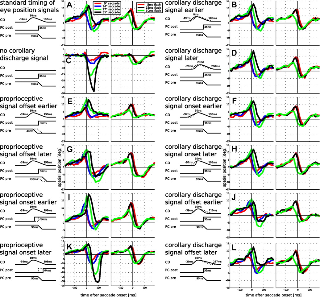
Parameter variations of the timing of the eye position signals for perisaccadic shift and flash length dependency using the non-head-centered model. The illustrations to the left of each panel show signal timings. Shown are times in which the signals reach one-half of their respective maxima and in which the CD signal peaks. Timings of the CD signal are relative to saccade onset; those of the proprioceptive signal are relative to saccade offset. A, The standard parameters of our model, same as in Figure 6, B and E. C, Outcomes with the same parameter set but without a CD signal. It can be seen that the CD signal is essential in explaining early mislocalizations. B, D–L, Variations of the timing parameters of the CD and proprioceptive signals. The offset time of the presaccadic proprioceptive signal is responsible for the amount of negative mislocalization after saccade onset. The longer it is active, the stronger the negative mislocalizations are (E, G). The onset of the postsaccadic proprioceptive signal influences the peak mislocalization around saccade onset (I, K). The onset of the CD signal controls the time the earliest mislocalizations appear (F, H). The offset of the CD signal influences mislocalizations around saccade onset (J, L). Note that, contrary to the proprioceptive signal timing (E, K), the effect of CD offset varies with saccade amplitude, with the most pronounced effect on the 35° saccade. It also affects late mislocalizations beyond 100 ms after saccade onset. The dotted lines indicate the timing of parameters in A.
As a first variation, we were interested in the effect of the CD signal. We tested this by running a simulation in which we turned off the CD completely (Fig. 11C). As a result, there were almost no positive mislocalizations but strong negative mislocalizations immediately after saccade onset. There are some positive mislocalizations for the 9° saccade (red line) but they only start as early as 30 ms before saccade onset. Since previous models claimed that perisaccadic shift can be explained without an anticipatory eye position signal (Pola, 2004; Teichert et al., 2010), we also tried to achieve the earliest possible mislocalizations without CD by shifting the updating of the proprioceptive signal to the earliest possible, although not plausible, time, which is immediately after saccade offset (data not shown). Indeed, this shifted the positive mislocalizations to start ∼50 ms before saccade onset, which is also the earliest time that mislocalizations started in the previous models by Pola (2004) and Teichert et al. (2010). An earlier misperception could only be achieved by a more pronounced visual latency or a longer (untypical) accumulation time in the decision neurons. Thus, according to our model, without the CD signal, it is not possible to explain the early mislocalizations that are observed in perisaccadic shift.
As far as the timing of the proprioceptive signal is concerned, it has recently been observed that proprioceptive eye position in LIP updates not immediately after saccade offset; rather complete updating can take as long as 150 ms (Xu et al., 2010). In our model parameters, we do not control the updating of the entire population but rather the offset and onset times of the signal at the presaccadic and postsaccadic eye positions. For the timing of the complete updating, see above (Decoding eye position). When we vary the time in which the presaccadic eye position signal turns off, we find that it primarily affects the amount of negative mislocalization after saccade offset (Fig. 11E,G). The later this offset time, the more negative the mislocalizations. As far as the timing of the onset of the new eye position signal at the postsaccadic eye position is concerned, we find primarily an influence on the peak mislocalizations around saccade onset. An earlier onset leads to stronger peak mislocalizations while a later onset leads to weaker peak mislocalizations as well as strong negative mislocalizations around saccade offset (Fig. 11I,K). A similar pattern can be observed, when the timing of the presaccadic and postsaccadic signals is varied simultaneously (data not shown). In sum, this suggests that differences in the amount of negative mislocalization between studies stem from intersubject variability in the timing of proprioceptive eye position signals.
Figure 11, B, D, F, H, J, and L, illustrates the effect of the timing of the CD signal. Varying the latency of the CD signal by ±10 ms does not change the observed effects (Fig. 11B,D). The effect of the onset time of the CD signal is straightforward: the earlier the CD starts, the earlier is the mislocalization (Fig. 11F,H). The influence of the offset time of the CD signal is more subtle. In contrast to the timing of the proprioceptive signal, it has little influence on the perisaccadic mislocalization for small saccade amplitudes (the red and blue lines in Fig. 11, J and L, are quite similar to those in Fig. 11A). However, long saccade amplitudes show an effect of CD offset timing on mislocalization (Fig. 11J,L, compare the peak mislocalizations of the black lines). Therefore, this parameter is partially responsible for the saturation behavior. This is in line with our earlier explanation of it (see above, Saccade amplitude dependency). Furthermore, the offset timing of the CD signal also affects late mislocalizations after 100 ms after saccade onset. Behavioral data sometimes show a second phase of positive mislocalization around that time (Fig. 6A). With a fast offset of the CD signal (Fig. 11J), these positive mislocalizations disappear, while with a longer decay they become stronger (Fig. 11L). In a monkey study, Jeffries et al. (2007) found almost no significant positive mislocalization presaccadically but a strong negative mislocalization after saccade onset. In their paper, they argued that this finding is inconsistent with a theory of a dampened eye position signal. Now, using our model, which invokes corollary discharge as well as proprioceptive eye position, we can show that these data (Fig. 12) can be well explained by a late updating of the proprioceptive signal (both offset of the presaccadic proprioceptive signal and onset of the postsaccadic proprioceptive signal 50 ms later) combined with a weaker CD signal (a factor of 0.4). The peak mislocalization in the model is a bit earlier than in the data. However, we did not intend to achieve an exact data fit by adjusting multiple parameters but rather provide an intuitive explanation for the peculiar observation of only negative mislocalization.

A later proprioception timing (offset and onset 50 ms later) combined with a weaker CD signal (by a factor of 0.4) results in a stronger negative mislocalization as it is reported by Jeffries et al. (2007) for a 14° saccade and 100 ms flash duration in a behavioral monkey study. The black dots are experimental data replotted from the study by Jeffries et al. (2007), their Figure 2a. The red line is model data.
Discussion
Various phenomena of perisaccadic perception have been addressed by different models (Hamker et al., 2011). Our model proposed here suggests that the mislocalization of brief flashes in total darkness can be explained by proprioceptive and corollary discharge eye position information. This is different for flashes in light that are perceived closer to the saccade target rather than into the direction of the saccade vector (Ross et al., 1997). This pattern has been explained such that a corollary discharge, which serves for attentional gain control, locally increases the visual capacity around the saccade target (Hamker et al., 2008). Such attentional gain increase appears weak when the flashed stimulus is much brighter than the perceptual threshold, but might affect localization even in total darkness when the flashed stimulus is close to threshold (Georg et al., 2008). Furthermore, localization can be made relative to visual references, which explains that the strong shift in saccade direction is not observed in those studies. Thus, the localization of brief flashes in total darkness and under illumination seem to rely on a different use of extraretinal signals. Our model discussed here is only intended for conditions of total darkness and not when references come into play, as for example by using two successively flashed stimuli (Sogo and Osaka, 2002).
Relationship to previous models
Previous models of perisaccadic shift determined the craniocentric position of a flashed stimulus by subtracting an extraretinal eye position-related signal from a retinal position estimate. While early models (Dassonville et al., 1992) took a static account, deducing the extraretinal signal from behavioral data and interpreting it as a sluggish eye position estimate, Pola (2004) and Teichert et al. (2010) introduced a realistically modeled retinal signal and temporal integration and, as a consequence, concluded that an anticipatory extraretinal signal is not necessary to explain the data. However, these models struggle with early onsets of mislocalization as well as with newer findings that show a saturation of mislocalization for larger saccade amplitudes (Van Wetter and Van Opstal, 2008). Our model does not explicitly compute a retinal position estimate.
Another crucial difference to previous models is the process of perceptual decision making that is not only biologically more plausible than a simple time average within a temporal window but imposes additional constraints with respect to the properties of eye position signals.
Eye position signals and their interaction
Recently, proprioceptive and corollary discharge signals became the focus of several investigations (Sommer and Wurtz, 2004; Wang et al., 2007). Yet many open questions remain about their functions. The proprioceptive information is assumed to have at least a long-term calibration role, but its short-term relevance is unclear, as for example the double-step experiment appears to be doable using the corollary discharge alone (Guthrie et al., 1983). Corollary discharge is hypothesized to mediate perisaccadic suppression as well as predictive remapping of visual receptive fields to anticipate the effects of saccadic eye movements (Wurtz, 2008), but so far only little work demonstrated its relevance for performing particular tasks (e.g., double step) (Sommer and Wurtz, 2008). The model of Teichert et al. (2010) and similarly the one of Pola (2004) suggest that such anticipatory extraretinal signals are not required to explain the data of perisaccadic shift. However, we show that the more plausible assumption of perceptual decision making by a neural integration process instead of time averaging in previous models lessens the influence of the late trace of the stimulus persistence, since neural integration depends on the temporal order within the activity trace. By switching off the CD signal in our model, we show that with reafferent eye position information alone no mislocalizations earlier than 50 ms before saccade onset can be achieved, which is also the earliest possible mislocalization in the model of Teichert et al. (2010), even with slow temporal dynamics. Thus, we conclude that corollary discharge plays an essential role in explaining perisaccadic shift.
This leads to interesting predictions. If the CD signal provides an anticipatory signal for spatial updating, then a microstimulation of cells in the CD pathway during fixation should also lead to a mislocalization of flashed stimuli in total darkness. Moreover, when we artificially dissociate between the planned saccade target as encoded by the CD signal and the actual landing point of the eye encoded by the proprioceptive signal, the model predicts that the saturation effect decreases for larger saccade undershoots. This could be systematically tested within a saccadic adaptation paradigm.
The role of gain fields and basis function networks
Several parietal areas including LIP show gain fields, a dependency of the neural response of cells with retinocentric receptive fields on eye position. It has been suggested that such gain fields are involved in coordinate transformation to combine signals across different reference frames (Zipser and Andersen, 1988; Denéve et al., 2001; Salinas and Abbott, 2001; Pouget et al., 2002). Similar gain fields have also been motivated in other studies of spatial perception such as spatial updating in double saccade tasks (Keith et al., 2010). However, little is known about how gain fields are involved in online control and perisaccadic space perception. Recently, it has been observed that gain fields update eye position very late after saccade end (Xu et al., 2010), which suggests that they are not involved in online control. Our model is consistent with these data and proposes that both, gain fields and (attentional) modulations by a corollary discharge together, could represent the spatial percept as discussed before. However, such a unified spatial percept requires a combination of a signal that codes eye position in the orbit and another one for eye displacement, and thus, it is necessary that both signals are encoded within the same reference frame. One possible solution would be to implicitly combine eye displacement information with eye position information by gain fields, while still relying on retinocentric receptive fields. Some evidence suggests that the FEF already relies on such an implicit coding format (Cassanello and Ferrera, 2007). As shown in our model, this would be sufficient to merge both stimulus representations into a unifying percept.
It is controversially debated whether there are true head-centered stimulus representations within LIP (Mullette-Gillman et al., 2005) and how different reference frames are used for localization and reach planning (McGuire and Sabes, 2009). By implementing a model version with an explicit head-centered representation as the output layer, we can show that perisaccadic shift can be explained equally well in both cases without any further changes in the model.
In conclusion, it has been argued that corollary discharge helps in establishing a stable representation of the external world (Wurtz, 2008). While future computational work is required to provide testable predictions for the role of corollary discharge in visual stability, our present work suggests that corollary discharge indeed plays a substantial role in stimulus localization, at least when no visual references are used.
Footnotes
This work was supported by the Federal Ministry of Education and Research Grant “Visuospatial Cognition” (Bundesministerium für Bildung und Forschung Grant 01GW0653). We thank Marc Zirnsak and Adam Morris for helpful comments on a previous version of this manuscript. Moreover, we are grateful to John Van Opstal and Michael E. Goldberg for providing us data to replot their main experimental observations.
- Correspondence should be addressed to Fred H. Hamker, Künstliche Intelligenz, Informatik, Technische Universität Chemnitz, Strasse der Nationen 62, 09107 Chemnitz, Germany. fred.hamker{at}informatik.tu-chemnitz.de


