

Abstract
Decisive contributions to our understanding of the mechanisms underlying the development of the nervous system have been made by studies performed at the level of single, identified cells in the fruit fly Drosophila. While all the motor neurons and glial cells in thoracic and abdominal segments of the Drosophila embryo have been individually identified, few of the interneurons, which comprise the vast majority of cells in the CNS, have been characterized at this level. We have applied a single cell labeling technique to carry out a detailed morphological characterization of the entire population of interneurons in abdominal segments A1–A7. Based on the definition of a set of spatial parameters specifying axonal projection patterns and cell body positions, we have identified 270 individual cell types as the complete hemisegmental set of interneurons and placed these in an interactive database. As well as facilitating analyses of developmental processes, this comprehensive set of data sheds light on the principles underlying the formation and organization of an entire segmental unit of the CNS.
Introduction
A major goal in developmental neurobiology is to understand how a large number of different types of neurons is generated and assembled into functional circuits. The embryonic ventral nerve cord of Drosophila, with its comparatively simple structure of repeated segmental units called neuromeres, has been one of the favored models used to address this problem. Apart from the availability of sophisticated genetic techniques and the convenient access to online data collections, one major advantage of this model is that analysis can be performed at the level of single, identified cells.
Each abdominal hemi-neuromere of the Drosophila embryo contains a stereotypic population of 30 stem cells [called neuroblasts (NBs)], which have been identified and characterized at a molecular level (Doe, 1992; Broadus et al., 1995). The largely invariant cellular lineages generated by these neuroblasts have also been described (Bossing et al., 1996; Schmidt et al., 1997; Schmid et al., 1999). While the labeling technique used to define individual neuroblast lineages reveals the composite axon projection patterns of the neural progeny, the axon morphology of individual neurons cannot generally be resolved.
Alternative methods have been used to determine the axonal and dendritic morphology of each of the 36 motor neurons that innervate body wall muscles in each hemisegment (Landgraf et al., 1997, 2003a) and the morphology of the 32 glial cells per hemineuromere that stem from NB lineages (Ito et al., 1995; Beckervordersandforth et al., 2008). However, only a few interneurons, which comprise the large majority of cells in each hemineuromere have been morphologically characterized as individuals. This has constrained our understanding of the mechanisms for cell fate specification in particular, since one of the key features of a neuron's identity is its axonal and dendritic morphology.
The current study has characterized the morphology of the complete population of interneurons in the late embryonic Drosophila abdominal nerve cord. A total of 954 cells have been individually labeled by juxtacellular DiI injection in abdominal neuromeres and grouped on the basis of morphological similarity, using a number of quantitative parameters. This has led to a collection of 270 groups or “cell types” that we believe represents a full hemisegmental set of abdominal interneurons. We have also identified the likely parental NB for each of these interneurons. Apart from its practical value in facilitating studies of neuron fate determination and mechanisms for axon guidance, this comprehensive set of data provides insights into principles of neuromere formation and organization. For example, we have been able to establish correlations between cell body position and axonal projection or between different aspects of axonal morphology. We have provided an interactive database, which will help to uncover further correlations, to identify cells sharing particular expression patterns and to search for potential interaction partners of identified neurons.
Materials and Methods
Fly stocks
Flies were raised at 18 or 25°C, depending on the desired developmental speed. We used the following stocks: Oregon R wild type; apterous-GAL4 (Calleja et al., 1996; kind gift from D. O'Keefe and J. B. Thomas); Mz360-eagle-Gal4 (Dittrich et al., 1997); UAS-CD8::GFP (from Bloomington Drosophila Stock Center at Indiana University).
Labeling of single interneurons
Preparation of capillaries.
Thin-walled glass capillaries with inner filaments (Science Products; GB 100 TF 8P) were drawn with a Sutter Instruments Model P97 puller. The tips of micropipettes are back filled with an ethanolic solution (0.1% in EtOH) of DiI (Invitrogen) and the shaft filled with 0.1 m LiCl.
DiI injection.
The procedure used for juxtacellular DiI labeling of individual neurons is a combination of those previously described by Merritt and Whitington (1995) and by Bossing and Technau (1994). For each round of injections, ∼15 embryos of either sex of the appropriate stage were manually dechorionated and mounted ventral side down on a coverslip coated with heptane glue. The embryos were filleted along the dorsal midline, flattened onto the coverslip, fixed for 15 min with 7.4% formaldehyde in PBS, washed 3–4 times with PBS and covered with PBS for DiI labeling. Neuronal cell bodies in the cortex region of the ventral nerve cord were viewed with a 50× or 100× water-immersion objective on a fixed stage upright microscope (Olympus BX 50 WI or Zeiss FS Axioskop). The tip of the microelectrode was brought into contact with a neuronal cell body using a Leitz micromanipulator and depolarizing current applied for a few seconds. The entire cell (including all fiber projections) became dye filled within a few seconds and was visualized using a Cy3 filter set. Up to 6 single cells per embryo or small groups of neighboring cells in different abdominal segments (A1–A7) were filled with DiI. The slide was then placed under a dissecting scope and the saline replaced by 7.4% formaldehyde in PBS for 15–20 min, followed by several washes in PBS. The labeled embryos were then individually subjected to photoconversion under the fluorescence microscope in the presence of 0.2% diaminobenzidene (DAB) in Tris buffer to give a permanent dark reaction product. The DAB was replaced with PBS several times. The preparations were cleared in 70% glycerol and covered with a coverslip for examination, imaging and storage.
Documentation of labeled cells
We recorded stacks of dorsal view images of each specimen on a motorized Zeiss Axioplan 2 with a z-distance of 0.5 μm and transformed them into QuickTime movie files. These movies were used to draw maximum projection images of all individual neurons. On the basis of the movies, we described the morphology of each labeled cell with the parameters summarized in Table 1 and Figure 1.
Parameters used to describe the morphology of the labeled cells (compare Fig. 1C,D)
Immunohistochemistry
Antibody stainings were performed following standard protocols. We used rabbit anti-GFP (1:500, Torrey Pines Biolabs) and biotin-conjugated anti-rabbit IgG (Jackson Immunoresearch Laboratories, 1:500).
Automatic generation of schematic representations of cell types
To develop a straightforward, standardized way of visualizing and comparing cell types, we made use of the ActionScript language within Adobe Flash, which allows shapes to be generated from code. A script within the database transformed the normalized positional values of a cell type (obtained from z-stack QuickTime movie files) into pixel values within a schematic representation of a segment and embedded these into the ActionScript code (see Fig. 4B), active in Adobe Acrobat or alternatively accessible under the following link: http://www.uni-mainz.de/FB/Biologie/Genetik/interneurons.html).
Results
Criteria used to define interneuron morphology
Juxtacellular DiI injections were performed on single neuronal cell bodies in abdominal neuromeres A1–A7 at late stage 16. At this embryonic stage, almost all labeled neurons were found to have extended an axon, although in many cases a growth cone was present, suggesting that the axon was still extending and may not have reached its final termination site. Previous analyses of neuroblast lineages in abdominal segments A1–A7 have uncovered little evidence of segmental differences in axon morphology of serially homologous neurons (Bossing et al., 1996; Schmidt et al., 1997). We have therefore assumed that these abdominal segments are identical to one another and have pooled data from different segments.
Representative examples of DiI-labeled interneurons are shown in Figure 1, A and B. We have addressed the following questions when characterizing the morphology of each individually labeled cell: Does the axon project ipsi- or contralateral to the cell body? If contralateral, does the axon lie in the anterior or posterior commissure? For contralateral axons, what is the position of the axon in the commissure in the anteroposterior (A-P) and dorsoventral (D-V) axes? For longitudinally projecting axons, what is the position of the axon in the mediolateral (M-L) and D-V axes? Do longitudinally projecting axons run anteriorly, posteriorly or in both directions? At what level in the A-P axis do longitudinally projecting axons terminate? Where are dendrites located? What is the location of the interneuron cell body in the A-P, M-L and D-V axes of the cortex?
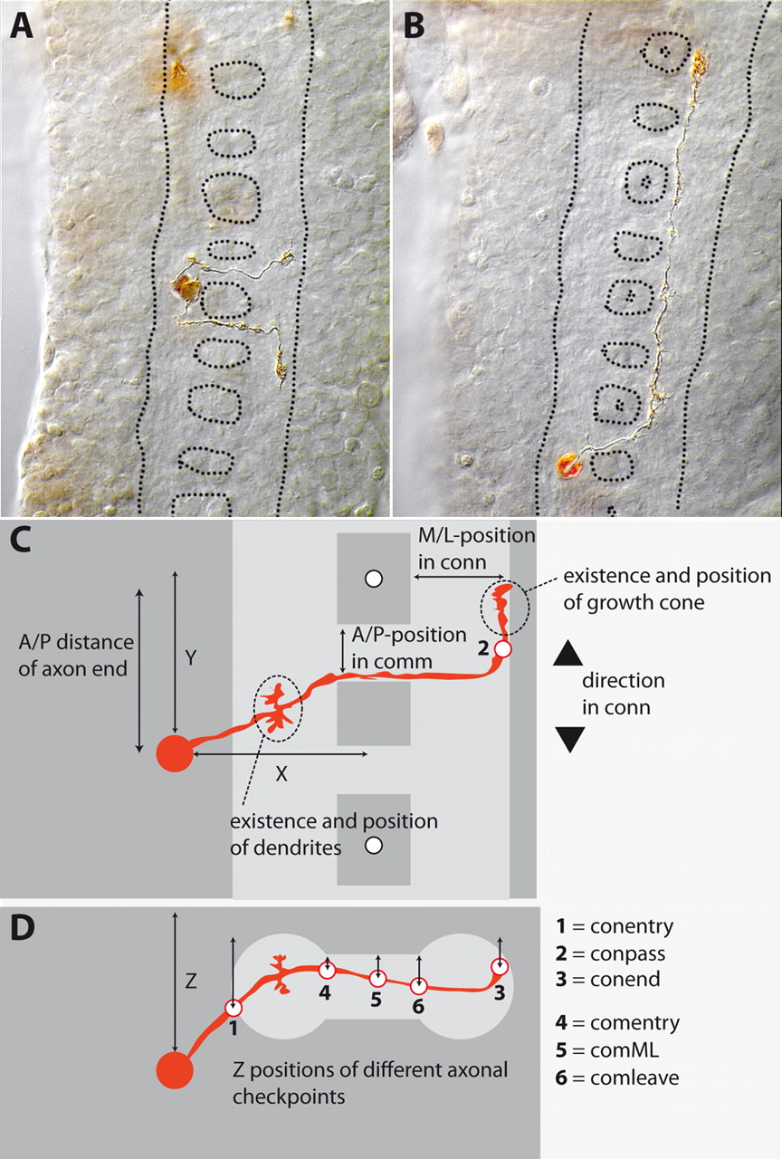
Two examples of DiI-labeled interneurons (A, B) and schematic presentation of the parameters that were measured (C, D). In A and B, views are from dorsal, anterior is up. Different focal planes have been manually combined in Photoshop. The neuropil is outlined by a dotted line. A, Two neighboring cells located close to the segment border. The more anterior cell (named X1Y3Z3copoIAnti3—for nomenclature, see “A naming system for interneurons”) crosses the midline through the PC and turns anterior in the connective, while the other cell (X1Y1Z3coanAPosti3) chooses the AC of the next posterior segment and turns posterior. B, An example of one of the longest ascending cell types labeled in the study (X1Y2Z3coanIAntv1). C, D, In C, view is from dorsal; in D, view is from posterior. The extent of approximately one neuromere is shown. The neuropil is shown in light gray and the cortex region in dark gray. In C, two white dots at the midline represent the dorsoventral channels, which mark the segment borders. For further details see Table 1.
Neuron morphology was defined by a total of 18 parameters (Fig. 1C,D; Table 1). For each labeled neuron, these parameters were measured from image stacks stored as QuickTime movies (see Material and Methods), and fed into a database.
In total, we labeled 954 interneurons. The spatial distribution of the labeled cells indicates that all cortical regions have been examined, although some locations have been sampled more frequently than others (Fig. 2).

Distribution of labeled cells. The cell body positions of all 954 labeled neurons are shown. Z represents the dorsoventral axis, X the mediolateral axis. To visualize 3D data and the number of labeled cells simultaneously, all Y (anterior–posterior axis) values have been summed for the respective X/Z positions. The shape of the cortex is indicated by the dark gray area. All cortex regions have been labeled, but the number of labeled cells varies between 1 and 40 among the individual positions.
Variability of neuronal morphology
We first sought to establish how much variability is present in the morphological measurements for a single type of interneuron. For this purpose, we used a number of cells that have been identified as individuals in previous studies. The first was an isolated apterous-Gal4-expressing cell situated dorsally, very close to the neuropil (Fig. 3A), which sends an ipsilateral projection anteriorly (dAP cell; Lundgren et al., 1995). We dye filled 19 dAP cells in apterous-Gal4, UAS-CD8::GFP embryos (Fig. 3D,E), using GFP expression to first locate the neuron cell body.

Neurons used to evaluate variability in the morphology and position of identified cells. A–C, Dorsal views of one to three abdominal segments. The midline is indicated with dotted lines. A, dAP neuron. Staining (brown) against GFP in apterous-Gal4, UAS-CD8::GFP embryos. At the lateral border of the neuropil, one cell per hemineuromere is stained. The cell body positions of 74 of these cells were measured and compared with 19 dAP cells that were individually labeled with DiI (see D–G). B, NB 7-3 interneurons. Upon labeling the NB 7-3 progenitor with DiI (at stage 7), the entire lineage (consisting of 4 cells) is marked in the late embryo (stage 16/17). While the motor neuron (M) projects posteriorly, the 3 interneurons (EW1–3) send their axons contralaterally as one bundle and only defasciculate after they have left the commissure (asterisk). We labeled 22 (random) EW neurons in eagle-Gal4, UAS-CD8::GFP embryos individually. C, TB neuron. Several cells have been labeled by DiI injections. The TB neuron (here pseudocolored in blue) stems from NB 1-2 and can be identified by its characteristic shape. We found it three times within our dataset. D–G, Variability of the dAP neuron. D, E, Examples of DiI labeling of individual apterous-Gal4, UAS-CD8::GFP expression dAP neurons. Dorsal view on flat preparations. The neuropil contour is outlined with white dots. We labeled 19 dAP cells to evaluate the variability of an identified cell's morphology and position. F, The outlines (blue) of all 19 individually labeled dAP neurons are combined (gray lines mark contours of neuropil and left cortex region). Note that cell body position is much more variable compared with fiber projections within the neuropil. G, Diagram of three d/v neuropil parameters (conentry, conpass, and conend; Fig. 1, Table 1). Each value varies ±15% around the average (bold red line). The point of connective entry (conentry) is more variable than the other two parameters due to its strong dependency on cell body position (which in the case of dAP is very close to the neuropil).
Figure 3, F and G, shows the variability we found for the 19 DiI-labeled dAP neurons: cell body positions vary approximately one cell diameter in each direction, while axon parameters in the neuropil (conentry, conpass, conend) vary within a range equivalent to 30% of the neuropil width. The variation of the anteroposterior (a/p) distance of the axon end (length of axon) has not been considered, as it probably reflects continuing axon extension at the time of labeling.
We then scored cell body positions and neuropil parameters of 74 dAP cells in embryos stained with an antibody against GFP. The values obtained were the same as for the DiI-labeled cells (according to t test; data not shown), indicating that the neuron injection procedure does not produce systematic artifacts in neuron morphology.
The second neuron type analyzed was the eagle-expressing EW interneurons. The eagle-positive NB 7-3 lineage consists of one motor neuron and three interneurons (EW1–3) (Higashijima et al., 1996) (Fig. 3B). The axons of the three EW neurons fasciculate and project through the posterior commissure (thereby giving an indication of variability in axon position within the commissure) and defasciculate in the contralateral connective. Variability in EW cell body position and axon position in the commissure is within the same range as for the dAP cells [±1 cell diameter and within a 30% dorsoventral (d/v) range in the commissure).
As a third example, we selected the TB neuron (Bossing et al., 1996), which is unambiguously identifiable from its unique morphology (Fig. 3C). Measurements on the 3 filled TB neurons in our study showed the same range of variability for axonal parameters as the other two cell types (between 8 and 30%), whereas the TB cell body position was relatively invariant.
On the basis of this analysis, we decided that axon position could lie within a 30% range for different labeled cells to be considered the same type of neuron. For cell body position, we allowed a maximum variability of 3 cell diameters (= one cell diameter variability around a center cell diameter). Our previous analysis of NB lineages had shown that cell body positions tend to be more variable for cells that are born late and therefore lie at more peripheral cortex positions compared with the earlier born cells, which are close to the neuropil (Schmidt et al., 1997). For some cells, we therefore increased the one cell diameter allowance to 1.5 cell diameters if all neuropil values fell within the 30% range.
Estimate of total number of interneuron types
To obtain an estimate of the total number of different interneuron types in our sample of labeled cells, we first separated these cells into three nonoverlapping populations: cells with ipsilateral projections (n = 289), cells that project through the anterior commissure (AC, n = 413) and cells that project through the posterior commissure (PC, n = 252).
Within each of these populations, we performed a complete unweighted hierarchical clustering using Euclidean distance with the help of the free software, Genesis 5.0, developed by Sturn et al. (2002). This analysis generated a tree with neurons sharing similar morphological parameter values grouped close to each other.
Since cluster analysis algorithms only measure similarity considering all parameters, we individually checked all groups within the database to make sure that the variability of each morphological criterion lies within the limit given by the examples described above (see “Variability of neuronal morphology”). This procedure of clustering and individual rechecking was repeated with the mean values of the groups of each reiteration until groups stopped fusing. After 5 rounds, this resulted in 270 groups/cell types, which corresponds well to an earlier estimate (based on cell body countings) of 250–300 interneurons in an abdominal hemisegment at early stage 17 (Rogulja-Ortmann et al., 2007). The fact that the number of distinguishable cell types is essentially equal to the estimated total number of interneurons indicates the absence of major morphological redundancy among cell types in an embryonic neuromere.
We compared the number of times each neuron type was filled with a statistical simulation in which 954 random numbers (= total number of labeled cells) were generated between 1 and 270 (= number of cell types). Averaging 10 of these simulations produces an almost Gaussian curve with a maximum of ∼3 cells per group and a prediction of 8 ± 2 unlabeled neuron types. The similarity between the predicted and actual curves leads us to conclude that our neuronal labeling missed only a small number of cell types (data not shown).
Visualization of neuronal morphology
We developed a scripting routine that transforms the numerical values of a cell type (as measured in image z-stacks) from the database into a schematic representation (see Materials and Methods). The procedure generates horizontal and frontal views of the cell (Fig. 4A,A′) from those data, enabling its shape and location within the cortex and neuropil to be readily visualized. Combinations of cell types that share particular morphological parameters can be simultaneously visualized, facilitating the search for correlations in neuronal morphology.

Example of how cell types are presented. A, Maximal projection drawings from QuickTime movies of 5 DiI-labeled cells that were grouped as one cell type. The neuropil is in light gray, the cortex in dark gray. A′, The corresponding schematic of this neuron type was automatically generated via Flash programming language ActionScript from the average values (Fig. 1) obtained from the five cells shown in A. Horizontal (left) and frontal (right) views show the position of the cell body and axon in the cortex and the neuropil. B, Flash App (active in Adobe Acrobat or alternatively accessible under the following link: http://www.uni-mainz.de/FB/Biologie/Genetik/interneurons.html) that allows rapid visualization of the cell types matching the criteria selected by the sliders. A click on a cell displays its individual characteristics. The code area allows the code name to be established for a particular cell or a cell can be displayed upon entering the code.
We have converted this script into an interactive Flash application (pdf-File in Fig. 4B or open http://www.uni-mainz.de/FB/Biologie/Genetik/interneurons.html). This application allows the rapid search and visualization of cell types sharing particular combinations of parameters (as selected by sliders). It further allows the display of the characteristics of individual cells, i.e., the schematics of neuron shape together with positional values for the cell body and axon, the neuronal code name (see below), the number of times the cell has been labeled, its putative parental neuroblast (predicted from a comparison with neuronal morphology in previously described neuroblast lineages), and molecular markers available to date.
A naming system for interneurons
We propose a five part naming system for interneurons. This system is based on neural morphology and generates a unique name for the large majority of the neuron types characterized in our study. The first part of the name indicates cell body position. The cortex is divided along each axis into three parts, generating 27 locations from X1Y1Z1 (medial, anterior and dorsal) to X3Y3Z3 (lateral, posterior and ventral) and the cell body is assigned to its nearest location. The second part of the name indicates whether the axon projects ipsilaterally (ipsi) or contralaterally (co). The third part indicates whether contralateral axons project into the anterior (ant) or posterior (p.o.) commissure, followed by a capital A (anterior third), I (intermediate third) or P (posterior third) to denote its position within the commissure. The fourth part denotes the direction taken by the axon within the connective: Ant (anterior), No (no obvious direction) or Post (posterior), followed by two digits that describe the position at which the axon terminates within the connective, again subdivided in thirds along the dorsoventral and mediolateral axes: d (dorsal), i (intermediate) and v (ventral) plus 1 (medial), 2 (intermediate) and 3 (lateral).
Within our dataset this code gives unique names to 199 cells, in 30 cases two cells share the same code, in 2 cases 3 cells have the same tag, in 1 case 4.
The code not only describes the morphology exactly enough to create a schematic image of a cell, it also helps to find a cell that exists in a preparation within our database. For example, if the cell of interest is located in the medial cortex (“X1”) close to the segment border (“Y4”) and sends an axon through the anterior commissure (“coant”) one would find the TB neuron (Fig. 3C) upon selecting the respective parameters in the CodeArea of the interactive database (Fig. 4B), active in Adobe Acrobat or alternatively accessible under the following link: http://www.uni-mainz.de/FB/Biologie/Genetik/interneurons.html).
General distribution of axon projections
Figure 5 gives an overview of the distribution of directions taken by axons in the neuropil. A total of 31% (n = 84; orange) of the cell types have ipsilaterally projecting axons while 69% cross the midline in the AC (43%, n = 117; blue) or PC (26%, n = 69; red). Approximately half of the cell types (48–55%) in each of these subsets of neurons send their axon in an anterior direction up the connectives, between 22% and 31% project neither anteriorly nor posteriorly and less than a quarter (21% to 23%) turn posteriorly. Only a few axons bifurcate and project both anteriorly and posteriorly. In such cases, the anterior branch is always present and is well developed, while the posterior branch is sometimes missing.

General distribution of axonal projections. This schematic shows a dorsal view on a neuromere summarizing the principal directions chosen by axons: 31% (n = 84, orange) stay ipsilateral, 43% (n = 117, blue) cross the midline via the AC, and 26% (n = 69, red) grow through the PC. In each class of neurons, approximately half of the axons (48–55%) turn anterior, less than a quarter (21–23%) turn posterior, and between 22 and 31% show no turn within the respective connective.
34 (= 3.4%) of the 988 labeled cells showed no sign of an axon and were not included into our database. These may represent neuroblasts or ganglion mother cells, neurons with axons that failed to label with DiI, neurons that had not projected an axon at the time of labeling or neurons that had withdrawn a previously formed axon.
Axon position in the commissures
Commissural axons show a strong tendency to remain in a constant dorsoventral position across the whole extent of the commissure: the correlation between the d/v position at entry into the commissure and at the exit point is 0.79 for all contralaterally projecting axons (Fig. 6A) and the entry and exit positions in the d/v axis differ by less than one third of thickness of the commissure for 93% of neurons (Fig. 6B). A few of the labeled axons (n = 7) show a difference in entry and exit position of between 50% and 63% of commissure thickness.

Axons in the commissures. A documents the correlation between an axon's d/v position at the entry into the commissure and when it exits the commissure (r = 0.79). B demonstrates that most axons (93%) cross the commissure with a d/v difference between entry and exit ≤30%. The numbers on top of the columns show actual axon numbers.
This behavior mirrors the tendency of commissural axons to remain in a constant anteroposterior position within the commissure, as noted in earlier studies (e.g., Bossing et al.,1996; Schmidt et al.,1997).
Axon position in the connectives
Observations of the position of longitudinally projecting axons in the current study support previous claims (Bossing et al., 1996; Schmidt et al., 1997; Landgraf et al., 2003b) that these axons maintain a relatively constant mediolateral position along the length of the connectives.
To analyze axon position within the connectives, we divided the connective into five parts along both the dorsoventral and mediolateral axes and determined which of these 25 positions each axon occupies (Fig. 7). If all types of neurons are considered, there is a relatively even distribution of axons across the connective (Fig. 7A) and the same applies to the subset of axons that project anteriorly (Fig. 7B). Axons that project posteriorly tend to lie in dorsal or lateral positions within the connectives (Fig. 7D): those posteriorly projecting axons that lie ipsilateral to their neuron cell body are mainly found in dorsal positions (Fig. 7H), whereas those that lie contralateral avoid medial positions (Fig. 7L). The axons of neurons that project neither anteriorly nor posteriorly (i.e., best candidates for local interneurons; see below, Projection neurons and local interneurons) are seldom found in lateral connective positions (Fig. 7C,G,K).

Positions of axons in the connectives. The dorsoventral and mediolateral axis of the connectives have both been divided into 5 parts resulting in 25 regions. The diagrams show how many axons (n = indicated by length of columns) reside in the respective regions for all axons (A–D), and directions (A, E, I) or subpopulations of axons [ipsilateral cells (ipsi cells, E–H) vs contralateral cells (contra cells, I–L)] and defined directions [anterior (B, F, J), no direction (C, G, K), and posterior direction (D, H, L)]. A shows that the entire neuron population is reasonably evenly distributed across the connectives (except for the borders that show less axons due to the round shape of the connective). Posterior projecting axons exhibit a clear avoidance of medial connective regions in the case of contralateral cells (L) and of more ventral positions in the case of ipsilateral axons (H). Contralateral axons that do not turn (K) are seldom found in the lateral two-fifths of the connective.
Relationship between axon position in commissures and connectives
There is a correlation between axon position in the dorsoventral axis of commissure and the position of the axon terminal in the dorsoventral axis of the connective (r = 0.67; for both commissures). Although the correlation is stronger (r = 0.77) for axons that terminate in the same segment as the neuron cell body, it is still clear for longer axons (r = 0.56) that end in distant segments.
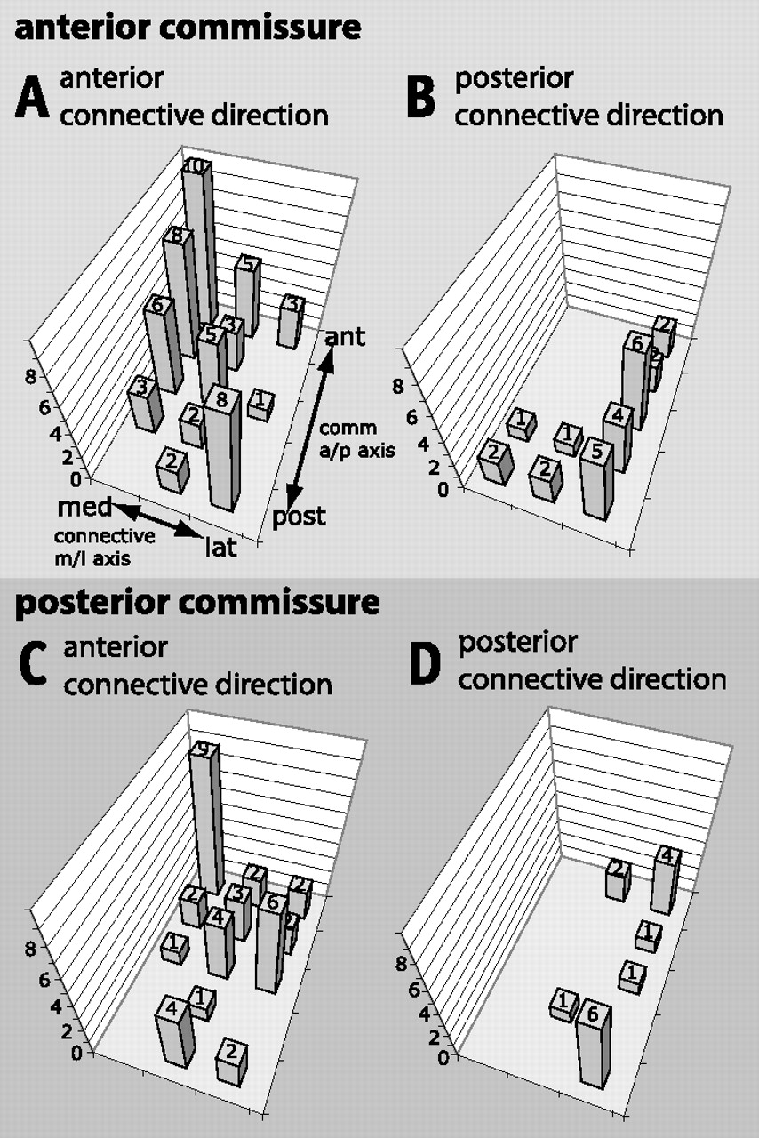
There is also a correlation between anteroposterior position within the commissure and mediolateral position within the connective (Fig. 8). In the case of axons that turn anteriorly, a more anterior position within the commissures correlates with a more medial position in the connective, whereas a more posterior position in the commissure correlates with a more lateral connective position (Fig. 8A,C). As noted above, axons that project posteriorly are found almost exclusively in lateral connective regions. These axons are relatively evenly distributed along the anteroposterior axis of the anterior commissure (Fig. 8B), but are clustered at the anterior and posterior limits of the posterior commissure (Fig. 8D).

Correlations between anteroposterior (a/p) position in the commissures and mediolateral (m/l) position in the connectives for contralaterally projecting neurons. The m/l axis of the connectives is divided into three parts; the a/p axis of the commissures is divided into five parts. A, Axons that project through the anterior region of the anterior commissure and turn anteriorly show a clear preference for medial connective regions while axons posterior in this commissure predominantly navigate through lateral connective regions. B, Posteriorly turning axons show a striking bias for more lateral bundles in the connective (compare Fig. 9). C, Anteriorly turning axons of the posterior commissure show a strong preference for anterior positions in the commissure and medial positions in the connective. There is no correlation between lateral position in connectives and posterior position in the commissures for this subset of neurons. D, Posteriorly directed axons that course in the posterior commissure occupy exclusively lateral regions of the connectives.
The relationship between the position of axons in the connectives and commissures is summarized in Figure 9. Commissure positions are divided into 9 groups (3 sections for each axis) and are symbolized as different colors that appear in the respective pie charts at the different connective positions. Here, the difference in mediolateral connective position between axons that turn anterior and those that turn posterior becomes obvious. All nine connective positions are used by anterior axons while 4 (AC) or 5 (PC) of the 6 medial positions are avoided by posterior axons.

Correlation between axonal positions in commissures and in connectives. This schematic shows a stylized 3D view summarizing the spatial organization of axonal projections. The commissures (anterior commissure in A and posterior commissure in B) have been divided into nine parts, represented by different colors. The regions into which axons navigate after leaving the commissures are represented by corresponding pie charts for axons turning anteriorly and posteriorly in the connective, respectively. It is apparent that medial connective regions are seldom used by posterior projections.
Projection neurons and local interneurons
Using the criterion that the longitudinal segment of the axon crosses the anterior or posterior neuromere border, 38% of the 270 different neuron types were judged to be projection neurons. Most of these neurons (63%) have contralateral cell bodies and of these, 78% cross in the anterior commissure.
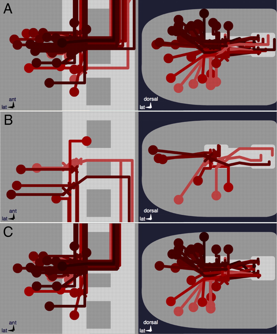
40 of the 103 projection neurons have axons that exceed the length of a neuromere. The vast majority of these cells (n = 33) turn anteriorly (ascending interneurons; Fig. 10A). Their axons generally end in the next segment (n = 23), but some extend up to 4 segments away. The 7 cells that project posteriorly (descending interneurons; Fig. 10B) can extend up to two segments away.

Projection neurons. A shows all 33 ascending cells that have an axon longer than one segment. All but one project through the AC. B shows the 7 descending cells with an axon longer than one segment. In C, 28 of the 33 ascending axons reside in the medial half of the connectives.
All of these projection neurons with relatively long axons occupy more central cortical positions: they are therefore likely to be early-born and some may be pioneer neurons. All except one of the contralateral ascending projection neurons (n = 19) use the anterior commissure, and most of them (n = 15) are found in the anterior region of the commissure. Furthermore, 28 of the 33 ascending interneurons occupy the medial region of the connectives (Fig. 10C).
62% of neuron types display axon projections that terminate within their segment of origin. These have been previously referred to as local interneurons (Schmid et al., 1999). Since an unknown fraction of these neurons may still be growing at the time of labeling we preferred a more restrictive definition and call cells “local interneurons” only if their axons do not turn either anteriorly or posteriorly (28%).
Relationship between cell body position and axonal projections
A correlation between the position of an interneuron's cell body and the choice of commissure by its axon has been previously suggested from an analysis of axon morphology as revealed in embryonic neuroblast lineages (Bossing et al., 1996; Schmidt et al., 1997; Schmid et al., 1999). The current study confirms this relationship: contralaterally projecting interneurons having their cell body in the anterior neuromere compartment send their axon through the anterior commissure, those in the posterior compartment select the posterior commissure (Fig. 11A). However, we have identified several neurons that do not follow this trend. Cell bodies of most of these neurons are found in the central cortex (being born early) of the posterior compartment and send their axon through the anterior commissure.

Relationship between cell body position and axonal projections. A, Contralateral projections of neurons with cell bodies in the anterior cortical compartment generally run through the anterior commissure, whereas the posterior commissure is preferred by neurons in posterior cortical regions. B, C, Cell body positions of the 69 cells with axons that terminate in the connectives without turning anteriorly or posteriorly (B, local interneurons), and of the 40 cells with axons longer than one segment (C, projection neurons). While most cell bodies in C lie close to the neuropil, the cells in B predominantly reside in positions closer to the cortex margin, typical for cells that are born late within their lineages and lie close to their parental NBs.
A further correlation apparent from our data exists between the time of neuron birth and axonal length: neurons lying in more marginal cortex positions, which are likely to be late-born, tend to have shorter axons (Fig. 11B) than neurons lying closer to the neuropil, which are likely to be early-born (Fig. 11C).
To establish whether cell body position correlates with other aspects of axonal morphology, we used a similar approach as in the section “Relationship between axon position in commissures and connectives.” Connectives and commissures were divided into 9 parts (3 sections for each axis) or 5 parts (along a single axis) and neurons that projected into each of these regions were grouped together (an example is given in Fig. 12).

An example of a search for relationships between cell body position and axonal projections. Cells were sorted according to similarity in a particular parameter of axon morphology, in this case d/v position within the commissure. A–E‴ show cells that project axons through anterior commissure; F–J‴ show cells that project through posterior commissure. The four columns represent all cells that match the respective criterion (yellow, letter without prime), only those cells with axons that turn anterior (orange, letter with one prime), cells with axons that do not turn (green, letter with two primes) or cells whose axons turn posterior (blue, letter with three primes). The number pairs in the corners display the respective number of cell types shown (upper number, bold) and the corresponding number of labels (lower number, regular). While many frames show no predominant cell body location, in some cases (e.g., B′, C‴, E‴, G′, H′, H‴) cells show strong preference for certain cortex areas. Another observation is that the d/v cortex position of cells is sometimes the opposite for the anterior and posterior commissures (compare B′ and C′ with G′ and H′ or B‴–D‴ with G‴–I‴).
It is evident from this analysis that there is no simple relationship between cell body position and any single feature of axon morphology. For example, the cell bodies of neurons that project axons into the lateral third region of the connective are scattered throughout the cortex (Fig. 13A).

Cells that project through lateral connective regions. A illustrates all 86 cells that send their projections into the lateral third of the connectives. B–L show subpopulations of these cells sorted according to their respective projection patterns.
However, relationships do become evident when certain combinations of axonal morphological features are considered. For example, the cell bodies of most of the neurons that project into the anterior commissure and in an anterior direction in the lateral region of the connective are grouped together (Fig. 13G).
One striking observation is that for contralateral neurons, the anterior and posterior commissures often show opposite correlations between cell body position and axon projections. Several examples illustrate this trend. Only 26% (9 of 34) neurons that project in the posterior fifth of the anterior commissure lie in a dorsal cortical position, whereas 87% (13 of 15) of cells that project in the same region of the posterior commissure lie in a dorsal position (Fig. 14A,B). Only 20% (5 of 25) of posteriorly projecting axons that cross in the anterior commissure have dorsal cell bodies, whereas 73% (11 of 15) of posteriorly projecting axons that cross in the posterior commissure have dorsal cell bodies (Fig. 14C,D).

Examples of inverse correlations between axons of different commissures. A, Of the 34 cells through the posterior fifth of the anterior commissure, 9 lie in dorsal cortex positions (26%). B, In contrast to A, 13 of 15 (87%) corresponding cells lie dorsal in the case of the posterior commissure. C, D, Five of 25 (20%) cells through anterior commissure and turning posterior in the connective have dorsal cell bodies (C) compared with 11 of 15 (73%) in the case of posterior commissure (D). E–H compare the contralateral cells in the ventral third of the cortex: 14 (= 28%) turn anterior (E) and 36 (= 72%) do not turn or turn posterior (F) after crossing through the anterior commissure. Conversely, 27 (= 71%) turn anterior (G) and 11 cells (= 29%) do not turn or turn posterior (H) after crossing through the posterior commissure. I shows all cells that project through the posterior fifth of the AC and turn posterior in the contralateral connective (red colors) and all cells that project through the anterior fifth of the PC and turn anterior (cyan). J depicts only those cells of the population shown in I which exhibit overlapping cortex positions. These cells are good candidates to stem from the same neuroblast (NB 4-1 or NB 5-2) but show inverse growth behavior in the connective: anterior and medial vs posterior and lateral.
While only 28% (14 of 50) of cells that lie in the ventral third of the cortex project anteriorly in the connective after crossing in the anterior commissure, 71% (27 of 38) of cells in the same cortical region project anteriorly after crossing in the posterior commissure (Fig. 14E–H). Figure 14, I and J, shows two subpopulation of neurons which share a similar position in the ventral cortex region but show fully divergent projection patterns.
Thus, neurons that lie in similar cortical regions, can show divergent patterns of axon growth. This divergence may be reflected in the choice of commissure, position within the commissure or direction of growth in the contralateral connectives.
Discussion
In the nematode worm Caenorhabditis elegans the entire nervous system (including sensory neurons) consists of ∼302 cells and the morphologies of all of the individual cell types have been described in detail (White et al., 1976). This knowledge has greatly facilitated investigations into both the development and function of the nervous system in this organism (for review, see Hobert, 2010). While neurons in Drosophila, as in C. elegans, are individually identifiable, the much larger number of neurons present in this organism might seem to make the task of obtaining a comparable, complete description of the nervous system unfeasible. However, the task becomes less daunting when one considers that the Drosophila nervous system is comprised of repeating segmental units—neuromeres. Whereas neuromeres of the brain, the gnathal, and the most posterior abdominal (A8–A10) segments are derived to various degrees, the thoracic (T1–T3) and anterior abdominal neuromeres (A1–A7) in the embryo are very similar and close to the ground state (T2, which does not require input from homeotic genes; Lewis, 1978). All motor neurons (Landgraf et al., 1997) and glial cells (Ito et al., 1995; Beckervordersandforth et al., 2008) in the thoracic and abdominal segments have already been individually identified and morphologically characterized. However, few of the interneurons, which are estimated to comprise ∼90% of the neurons in these segments, have been described on a morphological level. We applied a neural labeling technique, originally used to characterize the morphology of Drosophila sensory neurons (Merritt and Whitington, 1995), to perform a comprehensive analysis of the morphologies of all the interneurons in the abdominal ventral nerve cord of late stage wild type embryos.
Principles underlying neuromere organization
We found that 69% of the interneurons send their axons contralaterally while 31% stay ipsilateral. Around 50% of neurons have ascending axons while ∼20% have descending projections. The predominance of ascending projections corresponds with the function of interneurons in collecting and integrating information from sensory input and other interneurons and forwarding these toward the brain. While axons from abdominal interneurons generally terminate posterior to the brain, they may synapse with other interneurons that do project to the brain. Alternatively, or in addition, ascending dominance could be an evolutionary relic from short germband insects (in which segments are sequentially formed from anterior to posterior), reflecting the immaturity of more posterior segments at the time longitudinal pathways are pioneered.
We found that most of the projection neurons that are early-born (inferred from length of axon and position of cell body) occupy the anterior region of the anterior commissure. This suggests that the anterior commissure is established first and that new axons are added from anterior to posterior as the commissures develop. This conclusion is in agreement with previous data showing that axons of the prospective posterior commissure grow along preexisting axons of the anterior commissure, and that the two commissures are subsequently separated by midline glia (Klämbt et al., 1991; Hummel et al., 1999).
Our finding that ascending projection neurons largely occupy the medial domain of the connectives is consistent with the view that the establishment of longitudinal tracts occurs sequentially, from medial to lateral, through a series of distinct guidance events (Hidalgo and Booth, 2000; Wu et al., 2011). The establishment of the more medial longitudinal pathways in the connectives relies on the four (ipsilateral) pioneer axons vMP2, pCC and dMP2, MP1 (Hidalgo and Booth, 2000, and references therein), which interact with the longitudinal glia (Jacobs and Goodman, 1989a,b; Hidalgo et al., 1995; Kuzina et al., 2011). The identity of the cells that pioneer the most lateral pathways in Drosophila is still not known. To search for candidate lateral pioneers we applied the following criteria to the database: (1) axons are longer than half a segment and reach the next anterior or posterior segment, (2) axons reside medially in the lateral third of the connective, and (3) cell bodies lie close to the neuropil (early born cells). This resulted in the 4 candidate cells shown in Figure 15A.

Examples of uses of the database. A shows 4 candidate cells that pioneer the more lateral longitudinal tracts. The cells are selected when choosing the following combination of criteria: (1) axons being longer than half a segment and reaching the next anterior or posterior segment, (2) axons residing in a mediolateral connective region between 66% and 82%, (3) cell body positions close to the neuropil (x < 30%; z < 66%). B–D, Potentially connected populations of neurons. B is taken from the work of Zlatic et al. (2009) with the written permission of M. Zlatic and M. Bate, University of Cambridge, Cambridge, UK, and shows functionally different neuropil areas identified by the authors: the blue area is where most motor neuron dendrites arborize; in orange is the area where proprioceptive neurons terminate; green is the termination area of mechanosensory chordotonal organ neurons and yellow depicts the termination zone of nociceptive class II–IV multidendritic neurons. C shows the interneurons that project through PC and terminate in the dendritic field of motor neurons and are therefore good candidates for input neurons. D is the collection of all neurons that ipsi- and contralaterally pass through medial and ventral connective regions where nociceptive sensory neurons terminate.
Our study has shown that contralateral axons that turn posteriorly predominantly choose the lateral region. Positioning of the longitudinal tracts in the mediolateral axis is dependent on the combinatorial action of three Robo proteins that sense a repulsive Slit gradient (summarized by Dickson and Zou, 2010) with Robo2 being exclusively present in the lateral tracts (Rajagopalan et al., 2000; Evans and Bashaw, 2010; Spitzweck et al., 2010). This raises the interesting possibility that Robo2 may be involved in the selection of posterior versus anterior direction within the connectives.
Approximately 30% of the labeled neurons exhibit a short axon, which does not turn either anteriorly or posteriorly, but remains in the ipsi- or contralateral connective. These neurons are good candidates for local interneurons or neurosecretory cells. Such cells are predominantly found in more peripheral cortical regions (Fig. 11B), which are usually occupied by cells born late in a neuroblast lineage (Bossing et al., 1996; Kambadur et al., 1998). These findings therefore fit with a model in which neurons with long axons, including intersegmental projection neurons and motor neurons are early progeny of neuroblast divisions, whereas neurons with short axons, such as local interneurons are born later.
Except for birth-timing related proximo-distal positions of cell bodies in the cortex we did not detect obvious correlations between the spatial distribution of cell bodies and particular aspects of axonal navigation. This is in agreement with the fact that cells within embryonic NB lineages (that generally form dense clusters in the cortex) may assume very diverse fates (Bossing et al., 1996; Schmidt et al., 1997; Schmid et al., 1999).
An axon's choice of commissure is at least partly controlled by the repulsive function of wnt5 on the receptor Derailed (Bonkowsky et al., 1999; Yoshikawa et al., 2003) which is exclusively expressed by axons that build the AC (Wouda et al., 2008). The cortex position of the cells we found to project through AC is in good accordance with the published expression patterns of derailed. Nevertheless, there are several NB lineages known that send axons across both commissures: NBs 1-2, 4-1, 5-2, 5-3, 5-6, and 7-1 (Bossing et al., 1996; Schmidt et al., 1997). It will be interesting to determine the expression of derailed within lineages that project through both commissures.
A further question raised by this study is whether the opposite behavior of growth cones that cross the midline in the anterior and posterior commissures is due to intrinsic differences in the neurons involved and/or differences in the environment they encounter within the commissures. The embryonic CNS midline glia is directed to two alternative fates [anterior midline glia (AMG), posterior midline glia (PMG)] (Watson et al., 2011). During development AMG is in close contact to the AC and interacts with neurons under participation of Wrapper and Neurexin IV proteins (Stork et al., 2009; Wheeler et al., 2009) while PMG show much lower Wrapper levels and exclusively lie next to the PC. Although PMG function is not known, both glial cell populations are good candidates for differentially presenting guidance cues to axonal growth cones and/or modulating growth cone sensitivity.
Applications of the database
The data on axon morphology collected in this study is presented as an interactive application (Fig. 4B or http://www.uni-mainz.de/FB/Biologie/Genetik/interneurons.html), which allows easy searches, convenient display of multiple cell types sharing particular criteria and—since it can be opened in as many browser windows as demanded—simultaneous searches for different groups of cells.
In principle this database can be modified to incorporate further information of interest. For example, we have provided the most probable parental NB(s) for each cell. Further data, such as the function of a particular cell within the neural circuit or its fate during postembryonic development may be incorporated as they become available.
A particularly important extension of the database lies in the incorporation of gene expression data. It is only rarely possible to visualize the morphologies of individual cells in Gal4 lines that drive cytoplasmic markers in particular subpopulations of cells: either because axon morphology becomes obscured by the complexity of the expression pattern and/or the marker is too weak to reveal all structural details of these cells. The simultaneous use of Gal4 lines and targeted DiI injections, as performed in the current study, can allow axon morphology to be linked to patterns of gene expression at the level of individual neurons in both wild type and mutant backgrounds. This approach is particularly valuable in the embryonic context, since existing genetic methods for single cell labeling, such as MARCM (Lee and Luo, 1999) do not work effectively at this developmental stage.
Several studies have mapped the neuropilar regions in which the dendritic fields of motor neurons and the axon terminals of sensory neurons are found (Merritt and Whitington, 1995; Schrader and Merritt, 2000; Grueber et al., 2007; Zlatic et al., 2009; Wu et al., 2011). Combining this knowledge with information from the current study about interneuron axon morphology allows the identification of subsets of interneurons that may form synaptic connections with motor neurons or sensory neurons (Fig. 15B–D).
Footnotes
This work was supported by a grant from the DFG to G.M.T. We thank John Thomas (The Salk Institute, La Jolla, CA) and David O'Keefe (Fred Hutchinson Cancer Research Center, Seattle, WA) for gifts of fly strains.
- Correspondence should be addressed to Gerhard M. Technau, Institute of Genetics, University of Mainz, 55099 Mainz, Germany. technau{at}uni-mainz.de
This article is freely available online through the J Neurosci Open Choice option.


