

Abstract
Many of the neurons in early visual cortex are selective for the orientation of boundaries defined by first-order cues (luminance) as well as second-order cues (contrast, texture). The neural circuit mechanism underlying this selectivity is still unclear, but some studies have proposed that it emerges from spatial nonlinearities of subcortical Y cells. To understand how inputs from the Y-cell pathway might be pooled to generate cue-invariant receptive fields, we recorded visual responses from single neurons in cat Area 18 using linear multielectrode arrays. We measured responses to drifting and contrast-reversing luminance gratings as well as contrast modulation gratings. We found that a large fraction of these neurons have nonoriented responses to gratings, similar to those of subcortical Y cells: they respond at the second harmonic (F2) to high-spatial frequency contrast-reversing gratings and at the first harmonic (F1) to low-spatial frequency drifting gratings (“Y-cell signature”). For a given neuron, spatial frequency tuning for linear (F1) and nonlinear (F2) responses is quite distinct, similar to orientation-selective cue-invariant neurons. Also, these neurons respond to contrast modulation gratings with selectivity for the carrier (texture) spatial frequency and, in some cases, orientation. Their receptive field properties suggest that they could serve as building blocks for orientation-selective cue-invariant neurons. We propose a circuit model that combines ON- and OFF-center cortical Y-like cells in an unbalanced push–pull manner to generate orientation-selective, cue-invariant receptive fields.
SIGNIFICANCE STATEMENT A significant fraction of neurons in early visual cortex have specialized receptive fields that allow them to selectively respond to the orientation of boundaries that are invariant to the cue (luminance, contrast, texture, motion) that defines them. However, the neural mechanism to construct such versatile receptive fields remains unclear. Using multielectrode recording, we found a large fraction of neurons in early visual cortex with receptive fields not selective for orientation that have spatial nonlinearities like those of subcortical Y cells. These are strong candidates for building cue-invariant orientation-selective neurons; we present a neural circuit model that pools such neurons in an imbalanced “push–pull” manner, to generate orientation-selective cue-invariant receptive fields.
Introduction
A substantial fraction of neurons in the early visual cortex (Area 18) of cats respond in a cue-invariant manner to boundaries formed by first-order (luminance) or second-order (contrast, texture, motion) differences (Zhou and Baker, 1993; Tanaka and Ohzawa, 2006; Song and Baker, 2007; Gharat and Baker, 2012). Recently, neurons in the early visual cortex (V2) of nonhuman primates were also shown to respond cue invariantly to luminance- and contrast-defined boundaries (Li et al., 2014), with spatial selectivity to the carrier (texture) and envelope (modulator) of contrast boundaries that is very similar to previous findings in cat Area 18 (Mareschal and Baker, 1998a, 1999). Comparison of these primate V2 results with human psychophysics (Sutter et al., 1995; Dakin and Mareschal, 2000) suggests that these neurons could be the neural substrate for the perception of second-order boundaries.
However, the neural circuit underlying these highly specialized receptive fields, with cue-invariant selectivity for first- and second-order cues early in the visual pathway, is still unclear. The demonstration of carrier orientation selectivity in cat Area 18 cells suggested a cortical substrate for carrier processing (Mareschal and Baker, 1998a). More recent evidence suggests that cortical neurons could achieve such receptive field properties by pooling inputs from the subcortical Y-pathway (Demb et al., 2001a; Rosenberg et al., 2010; Rosenberg and Issa, 2011). Due to spatial nonlinearities, Y cells respond to first-order as well as second-order cues with selectivity for carrier (texture) spatial frequency and orientation similar to cortical neurons (Rosenberg et al., 2010). Thus, carrier processing for encoding second-order cues could take place in the retina, with the cue-invariant envelope selectivity arising in the cortex from the Y-cell input to the cortical neurons. A similar mechanism is also plausible in the primate visual system, since the parasol and upsilon cells in the retina also have Y-like receptive field properties (Petrusca et al., 2007; Crook et al., 2008). This challenges previous ideas that first- and second-order cues are processed independently (Smith and Ledgeway, 1997) and that second-order cues are encoded in higher extrastriate areas (Smith et al., 1998; El-Shamayleh and Movshon, 2011; Pan et al., 2012; An et al., 2014). Previous studies have extensively analyzed the pooling of subcortical X-pathway inputs in cat Area 17 to generate simple cell (linear, Gabor-like) receptive fields with a “push–pull” combination of ON- and OFF-center cells (Ferster, 1988; Hirsch et al., 1998; Martinez et al., 2005). However, Area 18 receives a majority of its lateral geniculate nucleus (LGN) input from the nonlinear Y-pathway, and it is unclear how these inputs are combined to generate receptive fields with precise selectivity for first-order as well as second-order cues.
To understand the cortical circuitry for second-order processing in the early visual pathway, we recorded single-unit activity from cat Area 18 using multielectrode arrays that can span all cortical layers. To reduce possible sampling biases due to manual searching with bar-shaped stimuli, we used a battery of grating measurements together with post hoc spike sorting. We found that a significant fraction of Area 18 neurons have receptive field properties similar to LGN Y cells, suggesting that these neurons form an intermediate stage between subcortical Y cells and orientation-selective cue-invariant neurons. Finally, we propose a cortical neural circuit model that combines signals from the ON and OFF cortical Y-like cells to generate receptive fields selective for orientation of both first- and second-order boundaries in a cue-invariant manner. Unlike the balanced push–pull model proposed for Area 17 neurons, this model has imbalanced push–pull, for example with ON inputs exerting a stronger effect than OFF inputs.
Materials and Methods
Animal preparation.
Our experimental procedures are explained in detail in our previous study (Gharat and Baker, 2012) and here are described briefly. Anesthesia was induced in adult cats of either sex with isoflurane/oxygen (3–5%) inhalation. Following intravenous cannulation, subsequent surgical anesthesia was obtained with intravenous propofol. A craniotomy and duratomy were performed (H-C A3/L4) for electrode placement in Area 18 (Tusa et al., 1979). During recording, the animal was anesthetized and paralyzed by the infusion of propofol (5.3 mg · kg−1 · h−1), fentanyl (7.4 μg · kg−1 · h−1), and gallamine triethiodide (10 mg · kg−1 · h−1), and a mixture of O2 and N2O (30:70 ratio) was delivered through a ventilator. Heart rate, EEG, body temperature, end-tidal CO2, blood oxygen, and airway pressure were monitored, with adjustments in ventilator stroke volume and anesthesia level as indicated. Neutral contact lenses and artificial pupils were positioned, and spectacle lenses of appropriate power were selected using a slit retinoscope. Back-projection of the optic discs onto a tangent screen allowed the estimation of area centralis positions. All of these procedures were approved by the Animal Care Committee of McGill University and are in accordance with the guidelines of the Canadian Council on Animal Care.
Visual stimuli.
Visual stimuli were presented on a gamma-corrected CRT monitor (20 inches, 640 × 480 pixels, 75 Hz, 36 cd/m2; FP1350, NEC) at a viewing distance of 57 cm. Stimuli were generated with an Apple Macintosh computer (MacPro, 2.66 GHz, 6 GB, MacOSX version 10.6.8) using custom MATLAB software with the Psychophysics Toolbox (Brainard, 1997; Kleiner et al., 2007). Drifting sinusoidal luminance gratings with a Michaelson contrast of 30% were used to measure the spatial frequency and orientation tuning of neurons.
Neurons were classified as X- or Y-like (see below) using contrast-reversing gratings with a higher contrast (70%) since nonlinear responses are often lower in amplitude. These gratings were also used to measure spatial frequency and orientation tuning, and spatial phase dependence, of nonlinear responses. In some cases, responses were also obtained to contrast modulation (CM) stimuli, which were composed from a stationary high spatial frequency sinusoidal grating (carrier, 70% contrast) whose contrast was modulated by a drifting low-spatial frequency sinusoidal grating (envelope, 100% modulation depth).
Extracellular recording.
Recordings were performed using multielectrodes (NeuroNexus), in most cases 32 channel (A1 × 32) linear arrays, but also sometimes 16 channel (A1 × 16) linear arrays and 16 channel (A4 × 4) tetrodes. Raw data signals were acquired with a Plexon Recorder (3 Hz to 8 kHz; sampling rate, 40 kHz). Signals from a selected channel with visually responsive single-unit or multiunit activity were used to guide the recording protocol. Spike times detected on this channel with a window discriminator were collected through a laboratory interface (ITC-18, Instrutech) and analyzed on-line to get tuning curves and peristimulus time histograms (PSTHs). Signals recorded from a small photocell placed over one corner of the CRT were used for temporal registration of stimuli and spikes, and to verify the absence of dropped frames.
Manually controlled visual stimuli (bars, spots) were used to determine the approximate receptive field location for multiunit activity on the monitored channel, so as to position the stimulus display to activate cells driven by the dominant eye (the nondominant eye was occluded). This procedure, rather than searching for single cells with bar-shaped stimuli, helped to ensure a less biased sample, including neurons lacking orientation selectivity. We attempted to insert multielectrodes perpendicular to the brain surface, so usually receptive field locations of neurons recorded on the other channels also fell on the display, enabling the simultaneous recording of useful visual responses of neurons on most channels. Drifting sinusoidal luminance gratings were presented to measure spatial frequency and orientation tuning. Each stimulus condition was interleaved with other conditions randomly and repeated 5–10 times. Contrast-reversing luminance gratings were then presented to measure nonlinear spatial summation. For all the spatial frequencies tested, either grating spatial phase or orientation was also varied. In some cases, we also measured responses to CM gratings. Multiunit activity across all channels during the experiment was analyzed to check whether recording sites were visually responsive. Once the recording protocol was finished, sometimes it was repeated on the nondominant eye, depending upon the quality of spike amplitude across channels.
Analysis.
Spike waveforms were carefully classified from the recorded data to isolate signals from single units, using Offline Sorter (version 3.3.3; Plexon) in earlier experiments, and later, Spikesorter (Swindale and Spacek, 2014) for sorting multichannel electrode data. On some datasets, sorting was performed with both types of software, and the results obtained were very similar. Only clearly sorted units were used for further analysis.
Responses of neurons to grating stimuli were accumulated as PSTHs (bin width, 13.3 ms; duration of each frame), which were used to calculate first-harmonic (F1) and second-harmonic (F2) responses. Neurons were classified as simple or complex type cells by measuring the ratio of first-harmonic modulation amplitude to mean, in response to the optimal drifting luminance grating of each neuron (Skottun et al., 1991). For orientation and spatial frequency tuning curves, the first-harmonic response rate was used for simple type cells, while the mean response rate was used for complex type cells.
The orientation selectivity of neurons was characterized with an “orientation bias” (OB) index (Leventhal et al., 2003), as follows:
 where Rk represents spontaneous-subtracted neuronal response at orientation θk. Orientation bias values range from zero (isotropic tuning) to unity (sharp tuning).
The degree to which neurons exhibited a binocular versus monocular response was summarized with a “binocularity index,” which was defined as the ratio of the average response to optimal drifting gratings in the nondominant eye to that in the dominant eye. The binocularity index ranges from zero (perfectly monocular) to unity (perfectly binocular).
To classify a neuron as X-like or Y-like we used a “nonlinearity index” (Hochstein and Shapley, 1976), which was defined as the maximum of the ratio of F2 response to F1 response. If at any spatial frequency, the second-harmonic response of a neuron was significantly greater than its first-harmonic component, it was classified as Y-like, otherwise as X-like. Note that only simple cells (AC/DC ratio >1) were further classified as X-like or Y-like, since complex cells respond nonlinearly (F2) within their luminance pass band and their first harmonic (F1) is very weak or absent. Spatial frequency tuning curves of linear (F1) and nonlinear (F2) responses were fit with a Gaussian function (DeAngelis et al., 1994) as follows:
 where k, SFopt, and α are free parameters, Ro is spontaneous activity, and R is the neuronal response at spatial frequency SF, with SFopt taken as the optimal spatial frequency.
Pearson's correlation coefficient between optimal linear and nonlinear spatial frequency was used to assess any relationship between the spatial tuning of a neuron for linear and nonlinear responses. The circular correlation (Berens, 2009) coefficient was used to assess the relationship between the optimal orientation of neurons for drifting and contrast-reversing gratings.
Results
Nonoriented receptive fields in cat Area 18
Previous single-unit studies of cat Area 18, including those in our laboratory, have primarily reported orientation-selective neurons. However, more recently, using multichannel microelectrodes with which we simultaneously record spikes from multiple neurons and analyze the data post hoc (see Materials and Methods), a significant fraction of neurons was found to have nonoriented receptive fields (Talebi and Baker, 2016).
Figure 1A shows example tuning curves of orientation-selective (left) and isotropic neurons (right), measured with drifting luminance gratings at the optimal spatial frequency of each neuron—these two neurons were simultaneously recorded from the same site on a multielectrode. We quantified the orientation selectivity of each neuron with an OB index (see Materials and Methods) which ranged from zero (isotropy) to unity (perfect selectivity). Neurons were classified as “non-ori” cells if OB was <0.2, which is the range found for LGN neurons (Rosenberg et al., 2010). The tuning curves in Figure 1A show examples of neurons classified as orientation selective (Fig. 1A, left; OB, 0.54) and non-ori (Fig. 1A, right; OB, 0.11).

Orientation tuning to drifting luminance gratings recorded with multielectrode arrays. A, Example tuning curves of an orientation-selective neuron (left) and a nonselective neuron (right), recorded simultaneously from the same site on a multielectrode. B, Orientation tuning curves of neurons recorded simultaneously with a 32-channel linear array inserted almost orthogonal to, and spanning, the cortical layers. Neurons showed varying degrees of orientation selectivity, with a large fraction lacking significant orientation selectivity (denoted by asterisks). The dotted box indicates the pair of neurons in A. C, Orientation selectivity of neurons is measured with an OB index, with higher values indicating greater orientation selectivity. Histogram shows the distribution of OB values of all 208 neurons in our Area 18 sample. Neurons with OB <0.2 are classified as non-orientation selective (LGN-like). More than one-third of these neurons (84 of 208 neurons) are non-orientation selective. D, Sorted spike waveforms for six example non-orientation-selective neurons recorded simultaneously.
Figure 1B shows an example of orientation tuning curves of neurons recorded simultaneously from a 32-channel linear array with recording sites separated by 100 μm. The array was inserted approximately perpendicular to the surface of the dura and lowered until most of the channels had spiking activity, so as to encompass all the cortical layers and to be approximately aligned with the columnar architecture. However, due to curvature of the brain beneath the dura, such electrode penetrations were not necessarily confined within an orientation column. The penetration shown in Figure 1B is an example of an evidently somewhat oblique penetration, traversing different orientation columns. Note that the span of depths with sorted neurons is 2.7 mm (28 channels), exceeding the anatomical thickness of gray matter in Area 18 (∼2 mm; Tusa et al., 1979). Note that non-ori neurons (Fig. 1B, asterisks) do not appear to be confined to particular layers, but rather are present at various depths spanning the gray matter and are intermixed with orientation-selective neurons. This is consistent with the findings of the study by Talebi and Baker (2016), who found neurons with nonoriented receptive field maps dispersed across all depths of Area 18. Figure 1C shows the distribution of orientation selectivity (OB values) of all the neurons that were recorded; more than one-third (84 of 208 neurons) were classified as non-ori. This histogram does not show a bimodal distribution indicating non-ori neurons as a separate class, which might seem to be in contradiction to the bimodal distribution seen in the similar histogram in Talebi and Baker (2016, their Fig. 6A) of OB values of Area 18 simple cells. However, note that here we calculated OB values from orientation tuning curves constructed by measuring responses at only 13 discrete orientations (separated by 30°), while Talebi and Baker (2016) measured OB values based on responses to a much larger number of orientations, simulated on a spatiotemporal receptive field map estimated by system identification. Their approach leads to much smoother tuning curves (Talebi and Baker, 2016, their Fig. 2D) and much lower OB values. However, the classic method of using responses to gratings can give high OB values due to limited sampling. So there is a strong possibility that even in our data non-ori cells might form a separate class from oriented receptive fields, but we fail to see it due to the limited sampling of orientations.
To assess whether these non-ori neurons behave like classic simple or complex type cells, we measured their AC/DC (modulated/mean response) ratio (Skottun et al., 1991; see Materials and Methods) for responses to optimized drifting gratings. The distribution of AC/DC ratios of non-ori neurons (Fig. 2B) shows that most (75 of 84 neurons) are simple type (ratios greater than unity). This suggests that most non-ori neurons have isotropic receptive fields with distinct concentric ON and OFF regions similar to LGN X and Y cells. We also find a few complex-like non-ori neurons (AC/DC ratios less than unity); these could be receiving input from the W pathway, some of whose neurons have mixed ON- and OFF-responding receptive fields (Stone et al., 1979).

Receptive field properties of non-orientation-selective neurons. A, Histogram showing the distribution of AC/DC (modulated/mean response) values of all 208 neurons in our Area 18 sample. B, Histogram showing the distribution of AC/DC (modulated/mean response) values for responses of non-orientation-selective neurons to drifting gratings. The majority of these neurons are simple type (AC/DC > unity). C, Scatterplot of binocularity index vs AC/DC ratio for non-orientation-selective neurons. There is no clear relationship between these two parameters. D, Histogram showing the distribution of binocularity indices for non-orientation-selective neurons. Most of these cells are monocular (index, <0.1), but approximately one-third are binocular.
In some cases (n = 38), we also assessed the degree of binocular response of the non-ori neurons, by separately measuring responses to each eye and taking their ratio as a “binocularity index” (see Materials and Methods). A purely monocular neuron should have an index close to zero, while a perfectly binocular neuron would have an index of unity. A histogram of these indices (Fig. 2D) shows that most of the non-ori neurons are monocular (25 of 38 neurons) but approximately one-third are binocular with index values as high as 0.93. A scatterplot (Fig. 2C) comparing binocularity indices and AC/DC ratios shows that there is no relationship between these two parameters (r = 0.0249, p = 0.882, n = 38).
One might wonder if these non-ori neurons are actually terminals of LGN afferent fibers. However, this is unlikely because we find them across all cortical depths (Fig. 1B), whereas LGN inputs terminate in layers 4 and 6 (LeVay and Gilbert, 1976). In addition, some of the non-ori cells are binocular (Fig. 2), which is characteristic of visual cortex (Hubel and Wiesel, 1962). Another potential concern is that poor spike sorting might inadvertently combine signals from several neurons with differing preferred orientations, giving an apparent lack of orientation tuning. Figure 1D shows sorted raw spike waveforms of six example non-ori neurons recorded in the penetration shown in Figure 1B. These sorted waveforms are clearly from single units, and hence the broad orientation tuning of these non-ori neurons is not due to contamination from multiunit activity. Furthermore, most of these cells give simple type (modulated) responses (Fig. 2B), whereas a mixture of neurons tuned to different orientations would give complex-like (unmodulated) responses.
Y-like spatial nonlinearities of non-ori receptive fields
Area 18 in the cat receives a strong direct input from the LGN, predominantly from Y cells, with much less input from X and W cells (Stone and Dreher, 1973; Dreher et al., 1980). Since these cortical non-ori neurons have orientation tuning similar to LGN cells, it seems likely that most of them receive direct or indirect input from LGN Y cells. Hence, we hypothesized that most cortical non-ori neurons should show the nonlinear spatial summation that is characteristic of LGN (and retinal) Y cells. Similar to previous studies of Y-type cells (Hochstein and Shapley, 1976; Demb et al., 2001a; Crook et al., 2008; Rosenberg et al., 2010), we measured the spatial properties of these neurons (n = 44) using drifting and contrast-reversing gratings.
Both X and Y type cells respond to drifting sinusoidal gratings at their fundamental temporal frequency (F1), which is indicative of linear processing. With contrast-reversing gratings, X cells also respond linearly (F1), but Y cells give second-harmonic (F2) responses (indicative of strong nonlinearity) at high spatial frequencies. We classified a neuron as Y like if its second-harmonic response component was significantly greater than the first harmonic to a contrast-reversing grating at any of the series of spatial frequencies tested (formalized as the nonlinearity index; see Materials and Methods); otherwise, it was classified as X like (Hochstein and Shapley, 1976).
Spatial frequency responses for a typical Y-like non-ori neuron are shown in Figure 3A. This neuron responded linearly (F1, red) to drifting gratings, with tuning for low spatial frequencies. But to contrast-reversing gratings the neuron responded nonlinearly (F2, blue) at high spatial frequencies outside the linear SF tuning range. This combination of results is the classic “Y-cell signature” (Hochstein and Shapley, 1976) for retinal and LGN Y cells.

Y-like non-orientation-selective neurons in Area 18. A, Spatial frequency responses of a typical non-orientation-selective neuron. F1 response to drifting gratings (black) is bandpass to low spatial frequencies. Similar to subcortical Y cells, this neuron responds nonlinearly at F2 (blue) to contrast-reversing high-spatial frequency gratings. B, PSTHs of the same neuron to contrast-reversing gratings (4 Hz) of low (0.1 cpd, left) and high (0.53 cpd, right) spatial frequencies. At low spatial frequency the neuron responds at the first harmonic (4 Hz) with periodic phase dependence, while at high spatial frequency it exhibits a second harmonic (8 Hz) across the full range of phases. C, Harmonic responses calculated from PSTHs in B as a function of spatial phase. The F1 response (black) is phase dependent with a clear null phase repeated every 180°, while the F2 response (blue) is phase independent. D, Distribution of nonlinearity indices of non-orientation-selective neurons. Most neurons are Y like (nonlinearity index, >1.0).
Figure 3B shows PSTH responses of this neuron to contrast-reversing gratings at two spatial frequencies, one within the linear SF range and the other in the nonlinear range. At a low SF (0.1 cycles per degree [cpd]; Fig. 3B, left), the neuron responded at the same temporal frequency as the grating (4 Hz), and this response depended on the spatial phase of the grating relative to the receptive field of the neuron, with a minimum (“null”) phase, all of which are indicative of linear spatial summation. But at a higher SF (0.53 cpd; Fig. 3B, right), the neuron gave a frequency-doubled response (8 Hz) that was phase independent, indicating nonlinear spatial summation. Figure 3C plots the first- and second-harmonic values calculated from the PSTHs in Figure 3B. The first-harmonic values depend on spatial phase, with a clear null phase repeated in 180° intervals, but the second-harmonic values are approximately constant with phase. Thus, this neuron showed all the spatial characteristics of a typical Y cell (Hochstein and Shapley, 1976). The distribution of spatial nonlinearity indices for the simple type non-ori neurons (Fig. 3D) were predominantly Y-like (36 of 44 neurons), but there were a few (8 of 44 neurons) X-like cells as well.
Linear and nonlinear spatial frequency relationships of Y-like cortical neurons
As shown in the previous section most of the cortical non-ori neurons have distinct linear and nonlinear SF tuning similar to those of retinal and LGN Y cells. Consequently, it seems a likely possibility that Area 18 non-ori neurons may be involved in cortical processing of second-order as well as first-order (luminance) stimuli. To further explore this possibility, we measured spatial tuning properties of non-ori neurons to compare with previously studied orientation-selective CM-responsive cortical neurons (Mareschal and Baker, 1999). Figure 4A–F shows linear and nonlinear SF tuning plots of six non-ori cells. Each cell has a bandpass-tuned nonlinear response (F2, blue) outside, and well above, the luminance pass band (F1, red). We fitted the data points with Gaussian functions (see Materials and Methods) to derive optimal SF values for linear (F1) and nonlinear (F2) tuning. A scatterplot of optimal SFs for linear versus nonlinear responses (Fig. 4G) shows that optimal SFs for F2 are always substantially higher than those for F1, with most of the neurons' values scattered around a 10:1 ratio line, and a weak correlation (r = 0.34) between optimal SFs for F1 and F2 for a given neuron. The distribution of F2/F1 ratios of optimal SFs (Fig. 4H) shows ratios ranging from 4.6 to 28, with a mean value of 11.3 (median, 8.7).

Linear and nonlinear spatial frequency tuning of cortical Y-like neurons. A–F, Spatial frequency tuning for six cortical Y-like neurons. F1 responses (black) of these neurons are bandpass tuned with selectivity for low spatial frequencies. F2 responses (blue) are bandpass tuned with selectivity for high spatial frequencies outside the luminance passband. G, Scatterplot of optimal spatial frequency for F2 responses vs that for F1 responses. All the points lie well above the 1:1 ratio line, indicating that the optimal spatial frequency of a given neuron for F2 is substantially higher than that for F1. H, Histogram showing ratios of optimal spatial frequency for F2 vs F1 (mean ratio, 11.3; median, 8.68).
A previous study (Mareschal and Baker, 1999) of orientation-selective neurons in Area 18 with contrast modulation gratings found similar results for linear and nonlinear spatial tuning. In that study, the ratio of optimal SF for the carrier of CM gratings (nonlinear) and drifting luminance gratings (linear) varied from 5 to 30, with a mean at ∼10. Similar ratios were also observed for CM response tunings in macaque V2 neurons (Li et al., 2014). Thus, cortical non-ori neurons have a relationship between linear and nonlinear SF tuning that is similar to that of orientation-selective CM-responsive neurons.
Orientation tuning of linear and nonlinear responses of Y-like cortical neurons
Some Area 18 neurons show pronounced orientation tuning for the high SF carrier of contrast modulation gratings (Mareschal and Baker, 1998a), which is independent of their orientation tuning for drifting luminance gratings. Hence, it was previously thought that receptive field subunits that detect the carrier are cortical, for example orientation-selective Area 17 neurons having high SF selectivity. However, Rosenberg et al. (2010) showed that even though LGN Y cells exhibit little or no selectivity for orientation of drifting gratings, some of them show pronounced orientation tuning for the carrier of CM gratings as well as for the nonlinear response to contrast-reversing high SF gratings. Thus, carrier orientation selectivity of CM-responsive Area 18 neurons might be inherited from afferent LGN Y cells. Therefore, we measured orientation tuning of nonlinear (F2) responses of Y-like cortical non-ori neurons to see whether some of them exhibit narrow tuning similar to that found for cortical oriented CM-responsive cells (Mareschal and Baker, 1998a; Rosenberg et al., 2010).
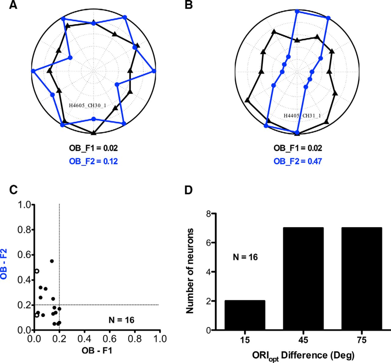
Figure 5, A and B, shows orientation tuning curves for the linear (F1, black) and nonlinear (F2, blue) responses of two non-ori Y-like neurons. The nonlinear (blue) tuning curves are symmetric because responses were collected for orientations from 0° to 180°, and the responses then mirrored about the origin. For the neuron in Figure 5A, the nonlinear response (blue) is not tuned (OB, 0.12) for the orientation of contrast-reversing gratings. For comparison, the responses of the same neuron to drifting gratings (black) are also shown; note that these linear responses have very small orientation bias (OB, 0.02) and are not direction selective. On the other hand, for the neuron in Figure 5B the nonlinear response (blue) is sharply tuned (OB, 0.47) for orientation while the linear response is not tuned (OB, 0.02). The scatterplot in Figure 5C shows the OB values of nonlinear against linear responses of neurons in this sample (n = 16). The linear responses (abscissa) all have OB values <0.2, as expected for non-ori neurons. However, for the nonlinear responses (ordinate), some of these neurons (6 of 16 neurons) have substantial orientation selectivity (OB values >0.2). We assessed the possibility of a systematic relationship between optimal orientation for linear (F1) responses and nonlinear (F2) responses. There was no significant circular correlation (Berens, 2009) between these optimal orientations for a given neuron (r = 0.0075, p = 0.9719, n = 16). The histogram in Figure 5D shows differences in preferred orientation for linear and nonlinear responses. The difference in preferred orientation for most neurons (14 of 16 neurons) was >30°. Thus, in this regard orientation tuning for nonlinear responses of cortical Y-like non-ori neurons is similar to that for LGN Y cells (Rosenberg et al., 2010) and for CM carrier tuning of cortical orientation-selective neurons (Mareschal and Baker, 1998a).

Linear and nonlinear orientation responses of Y-like non-ori neurons. A, B, Linear (F1, black) and nonlinear (F2, blue) orientation tuning plots of two Y-like non-ori neurons. One (A) is isotropic for orientation of nonlinear (F2) responses, while the other (B) has pronounced orientation tuning (OB, >0.2). C, Scatterplot showing comparison of orientation tuning for low spatial frequency drifting grating (F1) and high-spatial frequency contrast-reversing grating (F2). Higher OB values indicate greater selectivity. Open circles in the scatterplot correspond to the neurons in A and B. D, Histogram showing difference in optimal orientation for linear (F1) response and nonlinear (F2) response.
Responses of Y-like cortical neurons to second-order stimuli
Previous studies (Demb et al., 2001b; Rosenberg et al., 2010) demonstrated that retinal and LGN Y cells respond to CM gratings in addition to conventional luminance modulation gratings, suggesting that the Y-like non-ori cortical neurons might also be CM responsive. Figure 6, A and B, shows example snapshot images of CM gratings with a vertically oriented low-spatial frequency envelope that modulates the contrast of horizontal carrier gratings, the latter set at a lower carrier spatial frequency on the left (Fig. 6A), and higher frequency on the right (Fig. 6B). For measuring responses to CM gratings, we fixed the spatial frequency of the envelope at or near the optimal luminance SF (F1) and tested a series of carrier spatial frequencies outside the luminance passband of the neuron.

Responses of Y-like non-ori neurons to CM gratings. A, B, Two examples of contrast modulation stimuli with a vertically oriented low-spatial frequency envelope that modulates the contrast of horizontal carrier grating at low (A) or high (B) frequency. C–H, Spatial frequency tuning plots of six neurons to contrast modulation and luminance gratings. For a given neuron, the CM envelope spatial frequency was fixed at a low value within the luminance pass band (F1, black), and carrier spatial frequency was varied outside the luminance pass band. Neurons show bandpass tuning to CM gratings (orange), similar to their F2 response to contrast-reversing gratings (blue). I, Scatterplot of optimal spatial frequency of contrast reversing luminance gratings for F2 responses vs the optimal spatial frequency of CM carrier grating. J, Scatterplot showing spatial frequency bandwidth of the F2 response vs the bandwidth of CM carrier grating.
Figure 6C–H shows six non-ori neuron responses to CM gratings (orange) at a series of carrier SFs outside their luminance passbands (F1, black). These neurons show bandpass selectivity for the carrier of contrast modulation gratings (orange) that is very similar to their nonlinear SF tuning (F2, blue). The scatterplot in Figure 6I shows that the optimal spatial frequency for the carrier is very similar to that for nonlinear (F2) tuning (r = 0.9266, p = 0.0079, n = 6). As shown in the scatterplot in Figure 6J, the spatial frequency bandwidth for the carrier is often narrower than for nonlinear (F2) tuning. Furthermore, the optimal carrier spatial frequencies of these Y-like neurons fall within the same range (∼0.5–2.0 cpd, as those of cortical ori-selective CM-responsive neurons; Zhou and Baker, 1993; Mareschal and Baker, 1999; Rosenberg et al., 2010). These results suggest that responses to CM gratings and nonlinear responses to contrast-reversing gratings are elicited by a common nonlinear mechanism.
A possible cortical circuit using Y-pathway inputs to build cue-invariant receptive fields
We propose a cortical neural circuit model (Fig. 7B) that could generate cue-invariant orientation-selective receptive fields from responses of cortical Y-like cells. In this model, the responses of both ON- and OFF-center cortical neurons are combined in a “push–pull” manner (Ferster, 1988; Hirsch et al., 1998; Martinez et al., 2005): the ON subregions of an oriented receptive field receive excitatory input from ON-center cells and also inhibitory input from OFF-center cells, and vice versa for the OFF subregions. It is straightforward to see that this receptive field would be selective for the orientation of a luminance boundary. The centers of both ON- and OFF-type Y cells contain subunits (Demb et al., 2001a) that are excited by increases in texture contrast (i.e., give ON responses to contrast). Thus, if the push–pull between ON and OFF pathways is balanced, then the nonlinear responses to texture contrast will cancel out, and the neuron will be unresponsive to contrast boundaries. However, an imbalance of the ON and OFF pathways (Fig. 7B, wON not equal to wOFF) would enable a contrast boundary response. For example, if the ON pathway is stronger than the OFF pathway, then in the ON-subregion excitation from ON subunits will be stronger than inhibition from OFF subunits, and in the OFF subregion, inhibition from ON subunits will outweigh excitation from OFF subunits. Thus, the ON region would respond to an increase in texture contrast while the OFF region would respond to a decrease in texture contrast; thus, the receptive field as a whole would respond well to an oriented, periodic modulation of texture contrast.

Neural circuit model for cue-invariant receptive fields constructed from the Y pathway. A, The receptive field of a Y cell is modeled as a filter-rectify-filter (FRF) cascade. The first filter stage is composed of a bank of small DoG receptive fields corresponding to bipolar cells. The rectified outputs of these subunits are linearly pooled with DoG weighting, at a much larger spatial scale (Demb et al., 2001a). B, Receptive field of a cue-invariant cortical simple cell can be thought of as a pair of overlapping phase-aligned receptive fields, one constructed from the summation of ON-center inputs, and the other from OFF-center inputs. ON- and OFF-center Y-like cortical neurons are combined in a push–pull arrangement, such that the ON region of the cortical neuron receives excitatory input from ON-center cells and inhibitory input from OFF-center cells, and vice versa for the OFF region. This model will respond selectively to an oblique oriented luminance edge. But since the Y cells contain small nonlinear subunits, both ON and OFF types will be excited by the presence of texture, resulting in no net response. When the push–pull from ON and OFF pathways are unbalanced (e.g., stronger input from ON pathway), the nonlinear responses to texture no longer cancel, thereby enabling envelope orientation-selective responses to CM stimuli.
To demonstrate the tuning properties of this unbalanced neural circuit model, we constructed a computer simulation using a cascade of spatial filters. We modeled Y cells as summing rectified bipolar cell subunits (Enroth-Cugell and Robson, 1966; Demb et al., 2001a), as shown in Figure 7A. Outputs of ON- and OFF-type Y cells were combined in a push–pull manner, as shown in Figure 7B. Thus, this simulated model contains three filter stages corresponding to bipolar cells (ON and OFF center), Y cells (ON and OFF center), and a cortical orientation-selective simple cell, with half-wave rectification of the responses of each stage. We implicitly assume that receptive field properties of Y-type retinal ganglion cells (RGCs), LGN neurons, and cortical Y-like cells are not significantly different in their spatial receptive field properties. Bipolar cells were modeled as difference-of-Gaussian (DoG) filters with much wider surrounds compared with their centers and with center strengths outweighing surrounds (Dacey et al., 2000). Note that it is crucial for bipolar cell centers to be stronger than their surrounds to enable a linear response to low spatial frequencies (Dacey et al., 2000; Rosenberg and Issa, 2011). Outputs of these bipolar cell filters were rectified and pooled with DoG weighting, corresponding to RGC receptive fields. The center size of this DoG was set to be several times (10×) larger than the centers of the bipolar cell filters. ON-center Y cells were built by pooling ON-center bipolar cells, and OFF-center Y cells were built by pooling OFF-center bipolar cells (Demb et al., 1999). Finally, outputs of ON- and OFF-center Y cells were summed in a push–pull manner to build a cortical orientation-selective simple cell.
We measured responses of this model, with balanced as well as unbalanced push–pull to luminance modulation (LM) and CM gratings, to compare the spatial selectivity of the model to the selectivity of known cortical neurons (Mareschal and Baker, 1998b, 1999; Li et al., 2014). As shown in Figure 8A–C, the model with balanced push–pull responds selectively (spatial frequency and orientation) to LM gratings but fails to respond to CM gratings having a higher carrier spatial frequency (matched to the center size of bipolar cells). On the other hand, the model with unbalanced push–pull (Fig. 8D–F) not only responds selectively to LM gratings but also to CM gratings. Spatial frequency tuning (Fig. 8D, red) for the envelope of CM gratings is similar (though not identical) to that for LM gratings, and the carrier spatial frequency tuning (blue) is well above the luminance passband. In addition, this unbalanced model is also selective for similar orientation of LM gratings (Fig. 8E) and the envelope of CM gratings (Fig. 8F; i.e., form cue invariance). Note that in this scheme carrier selectivity arises from retinal stage (bipolar cell) filters, while the envelope selectivity emerges from cortical stage circuitry.

Spatial tuning of balanced and unbalanced push–pull model with Y-pathway inputs. A, Spatial frequency response of the model with balanced push–pull. Responses to luminance gratings (black) are bandpass tuned to low spatial frequencies, but the model does not respond to CM gratings (red, blue) with carrier spatial frequencies outside the luminance pass band. B, Balanced push–pull model shows orientation selectivity to drifting luminance gratings. C, Balanced push–pull model does not respond to CM gratings of any envelope orientation. D, Spatial frequency response of the model with unbalanced push–pull. Responses to luminance gratings are bandpass tuned to low spatial frequencies, as in A, but the model also responds to CM gratings with carrier spatial frequency selectivity (blue) outside luminance pass band and envelope selectivity (red) similar to that for LM gratings. E, Orientation tuning of the unbalanced push–pull model to drifting luminance gratings shows similar selectivity as B. F, Similar orientation tuning of the unbalanced push–pull model to the envelope of CM gratings.
Many CM-responsive neurons in cat Area 18 have broader envelope orientation tuning and a preference for lower envelope spatial frequencies, compared with their corresponding LM responses (Mareschal and Baker, 1999). In this model scheme, these differences arise from the very wide surrounds of the bipolar stage filters compared with their centers (Dacey et al., 2000). These surrounds make the luminance spatial frequency tuning of Y cells narrower by dampening responses to low spatial frequencies, thereby shifting the optimal spatial frequency slightly higher. However, for CM gratings at their optimal carrier spatial frequency (scale of bipolar cell centers), the surrounds of bipolar cells are too wide to detect the carrier. So, unlike the case with LM gratings, bipolar surrounds do not contribute to the selectivity for the envelope of CM gratings. This can result in subtle differences in spatial frequency tuning to LM gratings and envelopes of CM gratings in Y cells, with a preference for lower spatial frequencies of CM envelopes compared with LM gratings. These differences can be further increased by nonlinearities (expansive power law) at the outputs of Y cells and cortical ori cells and, thus, can give a difference in selectivity for luminance gratings and envelopes of CM gratings, as shown in Figure 8D–F.
Interestingly, CM-responsive Area 18 neurons show a pronounced selectivity for relative spatial phase between an LM grating and the envelope of a CM grating in a compound LM plus CM stimulus (Hutchinson et al., 2016). Therefore, we measured model responses to LM plus CM stimuli (Fig. 9A) for comparison. In the compound stimuli, the spatial frequencies of the LM gratings, and the envelope and carrier of the CM gratings, were set to optimal values, and the contrasts of the individual LM and CM gratings were adjusted such that the responses of the model to them were of equal strength, as in the experimental measurements of Hutchinson et al. (2016). Then the responses of the model were measured to LM plus CM gratings that were added at varying relative phases. When the model is made unbalanced, with wON > wOFF, its response (Fig. 9B) is selective for the relative phase in the compound stimuli, with the strongest response when the LM and CM are in phase (i.e., high luminance of LM aligned with high contrast of CM), in agreement with the results of the study by Hutchinson et al. (2016). This behavior arises because, in the Y-driven push–pull model, ON and OFF subregions for contrast detection are phase aligned with ON and OFF subregions for luminance detection.

Selectivity of the unbalanced push–pull model for relative spatial phase of luminance and contrast boundaries. A, LM plus CM compound gratings were constructed by linearly adding LM and CM gratings having identical spatial frequency and orientation. Compound stimuli are illustrated for “in-phase” condition (top), where high luminance of LM grating is phase aligned with a high contrast of a CM grating, and “antiphase” (bottom), where high luminance of LM grating is phase aligned with low contrast of CM grating. B, Responses of the unbalanced push–pull model to compound LM plus CM gratings with varying relative spatial phase. The model, with wON > wOFF, responds strongest when LM and CM gratings are phase aligned and weakest when they are in antiphase.
Discussion
Our results have demonstrated that a large fraction of the sampled population of cat Area 18 neurons have nonoriented Y-like receptive fields, which are present at different cortical depths intermixed with orientation-selective neurons and not evidently clustered in particular layers. These Y-like cortical neurons respond at the F2 to high-spatial frequency contrast-reversing gratings and at the F1 to low-spatial frequency drifting gratings (Y-cell signature; Enroth-Cugell and Robson, 1966; Hochstein and Shapley, 1976). The SF tunings of a given neuron for linear and nonlinear responses are quite distinct, with, on average, an ∼11-fold greater optimal SF for F2 than for F1. Furthermore, due to the nonlinearity of these neurons at high spatial frequencies, they also respond to CM patterns (second-order stimuli), with high selectivity for the spatial frequency of the CM carrier grating (texture).
Non-ori cells in cat Area 18
Early visual cortical areas are conventionally described as being characteristically composed of orientation-selective receptive fields. However, there have been some reports also finding a substantial fraction of LGN-like nonoriented receptive fields in the early mammalian visual cortex. For example, non-ori neurons have been found in primary visual cortex of macaque (Livingstone and Hubel, 1984; Ringach, 2002; Ringach et al., 2002), mouse (Bonin et al., 2011), and ferret (Chapman and Stryker, 1993), as well as in cat Area 17 (Dragoi et al., 2001; Hirsch et al., 2003). Earlier studies using single channel electrodes and bar-shaped search stimuli in cat Area 18 (Ferster and Jagadeesh, 1991; Mareschal and Baker, 1998a; Tanaka and Ohzawa, 2006) did not report nonoriented receptive fields. But a recent study (Talebi and Baker, 2016) in cat Area 18 using multichannel electrodes, in conjunction with post hoc data analysis (spike sorting) similar to ours, has reported a large proportion of nonoriented receptive fields estimated using system identification methods. We believe that using multielectrode arrays with post hoc spike sorting leads to less sampling bias compared with earlier approaches of sampling one neuron at a time with a single channel electrode. Furthermore, with earlier approaches, visual responsiveness of the neuron was typically assessed with moving bars. However, we have noticed that a moving bar is not a good stimulus for driving responses from these non-ori neurons—they are much better driven by flashing spots centered on their receptive fields, due to their comparatively strong surrounds. Thus, previous studies might have rarely found such neurons or failed to recognize their visual responsivity.
Nonlinear Y-like spatial summation
Here we have demonstrated that a significant fraction of neurons in early visual cortex of the cat have spatial receptive field properties similar to those of subcortical Y cells. These cortical neurons exhibit both linear and nonlinear spatial response properties, which are tuned for quite distinct spatial frequencies (Y cell signature; Hochstein and Shapley, 1976). Optimal spatial frequencies of our non-ori cortical neurons for linear and nonlinear responses (Fig. 4) are similar to those reported for retinal and LGN Y cells (Hochstein and Shapley, 1976; So and Shapley, 1979).
Ferster and Jagadeesh (1991) also described harmonic responses of orientation-selective simple cells in cat Area 18 to contrast-reversing gratings and found around half of their neuronal population to have Y-like spatial nonlinearities. However, they did not report the presence of non-ori Y-like cells. Spatial selectivity, such as the ratio of the preferred spatial frequency of linear and nonlinear responses, of their cell population is similar to the non-ori cells reported here except for their orientation selectivity.
Neural mechanism for building cue-invariant receptive fields
A significant fraction of Area 18 orientation-selective neurons are responsive to both first- and second-order visual stimuli, with the same preferred orientation to both (Zhou and Baker, 1993; Song and Baker, 2006; Gharat and Baker, 2012); that is, they are “form cue invariant” (Albright, 1992). Due to the additional selectivity of some of these neurons to carrier (texture) orientation, it was proposed that the neural substrate for subunits of Area 18 neurons was cortical in origin (Mareschal and Baker, 1998a). However, more recent evidence suggests that subcortical Y cells could provide a substrate for the carrier selectivity of cortical neurons (Demb et al., 2001a,b; Rosenberg et al., 2010), with the envelope selectivity arising from cortical circuitry. The cortical Y-like neurons that we have described are probably driven by LGN Y cells and could provide an intermediate stage for building cue-invariant orientation-selective receptive fields. First, they have carrier selectivity like cue-invariant neurons, but no orientation selectivity for drifting gratings, like Y cells. Unlike LGN cells, a significant fraction is binocular, which is also the case for some oriented CM-responsive cells (Tanaka and Ohzawa, 2006). Also, these Y-like neurons could provide both excitatory as well as inhibitory inputs to orientation-selective neurons - since input from the LGN to the cortex is only excitatory (Alonso et al., 2001), some sort of inhibitory interneuron would be necessary to construct a push–pull architecture for cortical receptive fields. Furthermore, the presence of some of these Y-like neurons in the top cortical layers suggests that they could also be projecting to higher-tier cortical areas along with the orientation-selective neurons.
Our model simulations predict that cortical neurons with unbalanced push–pull summation of Y-pathway inputs will be selective for the orientation of both luminance and texture boundaries, while the neurons that sum Y-pathway inputs with conventional balanced push–pull will only be selective for luminance boundaries. Furthermore, the unbalanced push–pull model is able to predict previously shown (Mareschal and Baker, 1998b, 1999; Li et al., 2014) spatial tuning properties of cortical neurons to LM and CM gratings, including systematic differences in tuning for LM gratings and envelopes of CM gratings.
This unbalanced push–pull model with a Y-pathway input is fundamentally different from the two-stream model proposed earlier (Zhou and Baker, 1993; Mareschal and Baker, 1998a) to explain the tuning properties of cortical neurons. In the two-stream model, selectivity for luminance and contrast processing arose separately, and only at the final stage were the outputs from these two streams summed. However, in this Y-pathway model, luminance and contrast cues are processed together all along the visual pathway beginning at the retina. In the two-stream model, the neural substrate for subunits that detect fine texture within contrast envelopes was thought to be Area 17 neurons (Mareschal and Baker, 1998a), but in this model it is retinal bipolar cells with rectified outputs. In Area 18, only approximately half of the orientation-selective neurons are responsive to both LM and CM gratings, while the remainder are only responsive to LM gratings, but not CM gratings (Zhou and Baker, 1993). This has been accounted for in the previous scheme by the presence or absence of input from a second stream for processing contrast boundaries. However, in this scheme a lack of response to contrast modulation would arise from a symmetrical push–pull, or from X- rather than Y-pathway inputs. Future studies could test this idea by assessing whether CM responsiveness of cortical neurons is correlated with their push–pull imbalance of Y-type inputs.
Implications for second-order processing in other mammals
While Y-type retinal ganglion cells were classically described in the cat, they have also been demonstrated in other mammals, including mouse (Schwartz et al., 2012) and guinea pig (Demb et al., 2001a). There have been doubts about the presence of a cell type homologous to Y cells in primates, as previous studies failed to clearly demonstrate Y-cell signature responses in retinal parasol cells (Petrusca et al., 2007). However Crook et al. (2008) clearly demonstrated that macaque retinal parasol cells have Y-like spatial nonlinearities. In view of our results, it seems likely that many of the non-ori neurons in area V1 of both mouse (Bonin et al., 2011) and monkey (Livingstone and Hubel, 1984; Ringach et al., 2002) might also have Y-like spatial nonlinearities inherited from subcortical Y-pathway inputs - this would be a future avenue of investigation.
Li et al. (2014) demonstrated that approximately one-third of neurons in macaque V2 respond to second-order stimuli in a form cue-invariant manner. Spatial tuning properties of these neurons to carriers and envelopes of CM gratings were qualitatively very similar to those in cat Area 18 neurons, differing principally in spatial scale. In addition, spatial frequency selectivity of V2 neurons (Li et al., 2014) for drifting luminance gratings and carriers of CM gratings is in a range that is similar to the spatial selectivity of retinal parasol cells (Crook et al., 2008) to drifting (F1) and contrast-reversing (F2) gratings, respectively. So, it is likely that, similar to cats, Y-like cortical cells are pooled to generate cue-invariant receptive fields in the early visual cortex of primates. Contrary to the view that second-order processing takes place in higher visual areas (Smith et al., 1998; El-Shamayleh and Movshon, 2011) and separate from first-order processing (Smith and Ledgeway, 1997; Larsson et al., 2006), it seems possible that all mammals including primates might have a common mechanism for processing second-order stimuli, involving the Y-cell pathway providing an early substrate for carrier tuning, and cortical circuitry with imbalanced push–pull for cue-invariant envelope tuning.
Footnotes
This work was supported by Canadian Institutes of Health Research Operating Grant MOP-119498 (to C.L.B.) and a Vanier Canada Graduate Scholarship (to A.G.). We thank Guangxing Li for providing the software for analyzing Plexon data files. We also thank Guangxing Li and Vargha Talebi for assistance with the experiments. In addition, we thank the NViDiA Corporation for the donation of a Tesla K40 GPU card through a NViDiA Hardware Grant.
The authors declare no competing financial interests.
- Correspondence should be addressed to Curtis L. Baker Jr., McGill Vision Research, MUHC Research Institute, 1650 Avenue Cedar, L11-521, Montreal, QC H3G 1A4, Canada. curtis.baker{at}mcgill.ca


