

Abstract
Curvature and tangential velocity of voluntary hand movements are constrained by an empirical relation known as the Two-Thirds Power Law. It has been argued that the law reflects the working of central control mechanisms, but it is not known whether these mechanisms are specific to the hand or shared also by other types of movement. Three experiments tested whether the power law applies to the smooth pursuit movements of the eye, which are controlled by distinct neural motor structures and a peculiar set of muscles. The first experiment showed that smooth pursuit of elliptic targets with various curvature–velocity relationships was most accurate when targets were compatible with the Two-Thirds Power Law. Tracking errors in all other cases reflected the fact that, irrespective of target kinematics, eye movements tended to comply with the law. Using only compatible targets, the second experiment demonstrated that kinematics per se cannot account for the pattern of pursuit errors. The third experiment showed that two-dimensional performance cannot be fully predicted on the basis of the performance observed when the horizontal and vertical components of the targets used in the first condition were tracked separately. We conclude that the Two-Thirds Power Law, in its various manifestations, reflects neural mechanisms common to otherwise distinct control modules.
- smooth pursuit eye movements
- two-dimensional tracking
- Lissajous motion
- curvature–velocity covariation
- Two-Thirds Power Law
- neural coding of direction
Many motor tasks can be performed equivalently with different combinations of rotations among body segments. Moreover, even when the trajectory of one endpoint is imposed, as in drawing, in principle its tangential velocity could vary in many ways. Yet only a limited number of solutions are actually implemented by the nervous system, suggesting that internal constraints force dynamic, kinematic, and geometrical variables to covary in a principled manner.
One such constraint, first described in free-hand movements (Viviani and Terzuolo, 1982; Lacquaniti et al., 1983; Viviani and Schneider, 1991), takes the form of an empirical relation, known as the Two-Thirds Power Law, between the shape and the kinematics of the motion. The law states that the radius of curvature (R) and the tangential velocity (V) satisfy the equation:
 where K is a velocity gain factor that depends on movement duration (Viviani, 1986). The parameter α takes negligible values if the trajectory does not have inflections (Viviani and Stucchi, 1992a). In adults, the value of the parameter β is very close to two thirds (Viviani and Schneider, 1991).
The neuromuscular system is forced to comply with the Two-Thirds Power Law even when an external template dictates the movement. When subjects track manually predictable (Viviani and Mounoud, 1990) or unpredictable (Viviani et al., 1987) targets, accuracy depends crucially on whether the target motion complies itself with the power law.
Several lines of evidence suggest that the law reflects the working of central motor modules. First, it was found (Massey et al., 1992) that the R–V covariation described by the equation above is present also when the trajectory is defined in isometric force-space, implying that the covariation is not implicit in the biomechanics of the limbs. Second, the Two-Thirds Power Law can be derived from a principle of optimal control (Minimum-Jerk Principle,Viviani and Flash, 1995) that is supposed to legislate motor planning at the central level (Hogan, 1984; Flash and Hogan, 1985; Flash, 1990). Third, visual and kinaesthetic perception of two-dimensional (2-D) targets is influenced by the R–V relationship in the stimuli (Viviani and Stucchi, 1989, 1992a,b; de’Sperati and Stucchi, 1995; Viviani et al., 1997). Finally, recent neurophysiological (Schwartz, 1992, 1994) and behavioral (Pellizzer et al., 1993) studies have suggested that the R–Vrelationship reflects a similar constraint present in the neural events coding movement direction in primary motor cortex (cf. Georgopoulos, 1995).
In spite of these advances, it is not known yet whether the Two-Thirds Power Law pertains to hand movements only or represents a more general constraint. We addressed this question by testing the behavior of the oculomotor system with two 2-D pursuit tracking experiments. The relevance of such a comparison has been argued in several studies on other constraining principles originally described for eye movements and was tested recently in the hand–arm system (Straumann et al., 1991; Hore et al., 1992, 1994; Miller et al., 1992; Crawford and Vilis, 1995; Soechting et al., 1995). The dynamic properties of the oculomotor plant (Robinson, 1981) are vastly different from those of the hand–arm complex. Moreover, different neural centers are involved in visuo-manual coordination and pursuit eye movements. Thus, demonstrating that oculomotor pursuit and visuo-manual pursuit exhibit the same peculiar limitations would deemphasize further the role of biomechanical factors. More importantly, it would provide direct evidence that the Two-Thirds Power Law reflects a general principle of neural dynamics shared by otherwise distinct motor centers.
If present, the R–V covariation may be a form of functional coupling, emerging most clearly when muscle synergies are engaged simultaneously in 2-D movements. Alternatively, it may be already inscribed in the dynamic characteristics of horizontal and vertical components. A third one-dimensional (1-D) pursuit tracking experiment was designed to address this point.
MATERIALS AND METHODS
Subjects. Nine staff members and students of the San Raffaele Vita-Salute University (five males, four females, between 19 and 37 years of age) volunteered for the experiments without being paid for their services. All subjects had normal vision. Only one had previous experience with eye movement recording. The protocol was approved by the ethical committee of the Institute. Informed consent was obtained from the participants.
Stimuli. In all cases, the target to be pursued was a white dot (radius = 0.17 mm) moving against the dark background of a computer screen (Hewlett Packard Ultra VGA, 17 in) at 114 cm from the subject’s eyes. At this distance, 1° of visual angle corresponds to 2 cm. Luminance was adjusted so that the stimulus had no appreciable flickering or persistence but was clearly visible in dark-adapted conditions. We tested three experimental conditions, each corresponding to a different type of target. In the first condition, the target moved clockwise along an elliptic trajectory defined by 1000 samples. The display rate was such that the motion period was always 3 sec. For a fixed length of its major semiaxis (Bx = 5.25°), an elliptic trajectory is defined uniquely by its aspect ratio By/Bx. Three ratios were tested: 0.25, 0.35, and 0.45. The corresponding eccentricities Σ = (1 − (By/Bx)2)1/2were 0.968, 0.936, and 0.893, respectively. The perimeters of the trajectory (in linear units) were 45.0, 47.1, and 49.5 cm. The ranges of variation of the radius R (in cm) were [0.65 − 42.3], [1.3 − 30.3], and [2.15 − 23.45]. The major axis of the ellipses was rotated clockwise by 45° (Fig.1A). The tangential velocityV of the target was a power function of the radius of curvature: V(t) =KR(t)1-β. The describes the mathematical procedure for specifying the componentsx = x(t) and y =y(t), so that the resulting motion exhibited the required covariation of R and V. Each trajectory (i.e., each value of Σ) was paired with seven values of β: 4/3, 7/6, 1, 5/6, 2/3, 1/2, 1/3, for a total of 21 stimuli differing in shape or distribution of velocity along the trajectory or both. As shown by the velocity components of the stimuli (Fig.1B), the value β = 2/3 yielded Lissajous motions [i.e., ellipses generated by composition of harmonic functions (Viviani and Cenzato, 1985)]. Figure 1C illustrates the time course of the tangential velocity over a cycle for Σ = 0.936 and all values of β. When β >1, velocity was maximum at the poles of the trajectory. When β = 1, velocity was constant. When β < 1, velocity was maximum at the points of minimum curvature (curvature is the inverse of the radius of curvature). The polar plot in Figure1D illustrates how velocity varied along the trajectory for two values of β when the eccentricity was set at Σ = 0.936. Data in the first experimental condition were obtained from nine subjects.

Shape and kinematics of the targets, first experimental condition. A, Trajectories; the major axis of the trajectory was the same in all cases. B, Horizontal (HOR) and vertical (VERT) velocity components of the target as a function of time for Σ = 0.936 and each value of β. For β = 2/3, the components are sine and cosine functions (Lissajous movement). Only one cycle is shown. C, Tangential velocities corresponding to the components in B (the vertical spacing between traces is arbitrary). Time and velocity calibration bars are common to B and C.D, Polar plot of the tangential velocity distribution along the trajectory for Σ = 0.936 and the extreme values of β. The velocity at each trajectory point A is proportional to the length of the segment A–B.
In the second experimental condition, only seven targets were presented. Their velocity functions V =V(t) were the same as those for the subset of stimuli in the first condition with the highest eccentricity (Σ = 0.968). With a mathematical procedure detailed in the , the components x = x(t) andy = y(t) of each target were computed in such a way that (1) its tangential velocity coincided with the function V that the target was associated with; (2) the motion complied with the Two-Thirds Power Law; and (3) the perimeter of the trajectory was the same as that of the corresponding target in the first condition. Requirements 1 and 3 imply that targets also had the same period as in the first experiment. Requirements 1 and 2 imply that in all but one case (β = 2/3), the trajectories were not ellipses (see Fig. 8, right column). Data were obtained from one female and two male subjects who already had been tested in the first condition.

Tracking compatible targets, second experimental condition. Left column, Tangential velocity and derivatives of the cartesian components. Averages and 95% confidence bands calculated on three subjects; same format as in Figure 5. Target tangential velocities are identical to those in the first condition for Σ = 0.968 and for the associated β (A, β = 4/3;B, β = 1; C, β = 2/3;D, β = 1/3). The velocity of the components depended on the trajectory of the stimuli (right column) and were not the same as those in the first condition. By design, all stimuli in this condition complied with the Two-Thirds Power Law.
In the third experimental condition, targets were 1-D. We presented separately, in random order, the horizontal and vertical components of the stimuli of the first condition corresponding to Σ = 0.968 (14 stimuli in total). Data were obtained from three male subjects who already had been tested in the first condition.
Eye movement recording. Horizontal and vertical components of eye position were recorded monocularly with the scleral search coil technique (Robinson, 1963; Collewijn et al., 1975). Within the normal oculomotor range, the recording device (EPM520, Skalar Medical) has a nominal accuracy of < 1 min. Position signals were low-pass-filtered (cutoff frequency, 300 Hz), sampled (16-bit accuracy, sampling frequency, 500 Hz per channel), calibrated (see below), and stored for subsequent processing.
Experimental procedure. Experiments took place in a dark room. The subject was seated inside the recording device. The head was immobilized with the help of a forehead abutment and a bite-board molded individually with condensation silicone. Head position was adjusted so that the recorded eye was at the center of the magnetic field and aligned with the center of the screen. Stimuli were viewed monocularly with the dominant eye. The other eye was fitted with the search coil and patched to prevent blurring caused by the overproduction of tears. Before fitting the search coil, the sclera was lightly anesthetized with a local application of oxibuprocaine chlorydrate (Novesine 0.4%, Sandoz), and a small amount of adhesive solution (Idroxy-Propil-Metil-Cellulosa, Cel 4000, Bruschettini, Genova, I) was applied to the search coil. A 2–3 min adaptation period was allowed after fitting the search coil. If the subject reported discomfort during this period or thereafter, the experiment was terminated immediately. The experimental session was preceded by a calibration phase in which the subject had to fixate sequentially 25 targets arranged as a 5 × 5 rectangular matrix (size, 10.5° × 7.75°). Calibration targets were white circles (radius, 0.1°) centered on an orthogonal cross (width, 0.4°). Individual fixations or the entire calibration could be repeated if necessary.
The three conditions were administered in separate sessions, at least 1 week apart. A session consisted of an uninterrupted randomized sequence of trials, one for each target type. Trials were initiated by the experimenter 1 sec after an acoustic warning signal. Ten stimulus cycles were presented in each trial, the task being to follow the target as accurately as possible for the duration of the recording (30 sec). The interval between trials was at least 15 sec. At the end of the recording period, both the calibrated trace and itsx–y components were compared with the corresponding target data. Trials contaminated by eyeblinks were repeated. Sessions lasted ∼20 min, including calibration. At the end, the eye was washed with Collyrium and checked.
Data analysis. Raw data were calibrated by evaluating the parameters of 2 third-degree polynomials X =FX(x,y) andY =FY(x,y) that best mapped (in the least-square sense) the recorded calibration grid into the theoretical grid. Calibrated position data were expressed in degrees, using the screen as a reference. The first cycle of each trial was always discarded. Velocity and acceleration components were computed by differentiating the position data with a 15-point digital filter (FIR,Rabiner and Gold, 1975). Saccades and smooth pursuit phases in the calibrated trace (heretofore, tracking movement) were analyzed separately. Saccades were identified automatically as periods in which the tangential velocity exceeded 15°/sec for >6 msec. The smooth pursuit component was defined as what is left of the tracking movement after removing both the saccades and the 30 msec segments before and after each saccade. This phase of the processing was controlled interactively, taking into consideration position and velocity traces.
RESULTS
Two-dimensional tracking of stimuli with variousR–V relationships
Whatever the stimulus type, a substantial number of saccades were interspersed within the smooth phase of the response. Typical mixtures of the two tracking components are illustrated in Figure2 with representative recordings in two kinematic conditions (one subject). The β value of the target had a consistent effect on the distribution of tracking errors along the trajectory. Eye position records (POS) show that, in general, the form of the target was restituted rather faithfully, the largest errors occurring at the points of maximum curvature when β >1. By contrast, there were conspicuous tracking failures in the kinematic domain. In particular, the tangential velocity of the smooth response (VEL) failed to match peak values of target velocity when they occurred in the high-curvature portions of the trajectory (e.g., for β = 4/3, top velocity plot). Note that the limiting factor was not the value of the tangential velocity per se, which remained within the normal dynamic range of operation of the smooth pursuit system. In fact, the same target velocity that triggered many compensatory saccades when the curvature was high (as in the top traces) could be dealt with effectively when it occurred in regions of lower curvature (e.g., for β = 1/3, bottom velocity plot). This point will be expanded later.

Tracking eye movements, first experimental condition. Left, The four bottom traces inA (β = 4/3) and B (β = 1/3) show representative examples of the horizontal and vertical position of the target (TARG) and the tracking eye movements (TRACK) for Σ = 0.936 (for clarity, only 6 cycles are plotted). HOR, Horizontal component;VERT, vertical component. Movement directions for both components are indicated by arrows (RW, Rightward; LW, leftward; UW, upward;DW, downward). In the four top traces, tracking components were dissociated into saccadic (SACC) and smooth pursuit (SP) contributions. Right, Representative examples of tracking trajectories (POS, including both saccades and smooth pursuit) and the polar plot of the smooth pursuit velocity (VEL), superimposed to the corresponding curves of trajectory and velocity for the target (thick continuous line). Target shapes were reproduced fairly accurately. Target velocity was generally underestimated.
The top panel in Figure 3 shows that, irrespective of the eccentricity of the trajectory, the number of saccades in a cycle (averaged over all subjects) was minimum when the stimulus complied with the Two-Thirds Power Law. The value of β also determined the tracking effectiveness of the smooth pursuit component estimated through a global smooth pursuit mismatch index (Fig. 3, middle panel). Considering the smooth pursuit phases between two successive saccades, the index was defined as the difference between the absolute retinal position error (RPE) immediately before the second and immediately after the first saccade (averaged over all phases). Thus, it measured the increase of the distance of the gaze with respect to the target during the pursuit. The index attained a well-defined minimum (maximum effectiveness) between β = 2/3 and β = 5/6. Most saccades were compensatory, intervening whenever the RPE became too large. We used the average difference between the RPE immediately before and after each saccade (saccadic mismatch index, Fig. 3,bottom panel) to estimate the global contribution to tracking by the saccadic system. Because a good correlation exists between the RPE and the extent of saccadic compensation, the index also afforded an average measure of saccade size. As expected, the least amount of saccadic compensation occurred when smooth pursuit was most effective.

Top panel, Mean and 95% confidence interval of the number of saccades per cycle. Middle andbottom panels, Mismatch index (mean and 95% confidence interval) for smooth pursuit and saccades, respectively. Results for all targets and all subjects in the first experimental condition. Gaze-target distance never became zero during smooth pursuit (positive values of the smooth pursuit index). Most saccades were compensatory (positive values of the index). Between β = 5/6 and β = 2/3, smooth pursuit was most effective, and the contribution of compensatory saccades was smallest.
The distribution of the RPE along the movement cycle is shown in the polar plots of Figure 4. We divided the target cycle into 16 angular sectors corresponding to an equal number of samples, and we computed the average RPE within each sector, pooling data from all subjects. The 95% confidence intervals computed from individual means (radial bars) estimate between-subject variability within each sector. The results indicate that pursuit errors were particularly large both when velocity increased at the points of high curvature (e.g., at the poles for β = 4/3) and when velocity increased at the points of low curvature more than predicted by the Two-Thirds Power Law (e.g., in the flatter parts of the trajectory for β = 1/3). The asymmetry in the distribution of RPE was less marked at lower eccentricities, i.e., for trajectories with smaller excursions of curvature values.

Polar plots of the average retinal position error (RPE) along the trajectory for the indicated values of β at Σ = 0.968. Instantaneous values of the RPE for all subjects were averaged within each of 16 angular sectors. The average RPE within each sector is proportional to the radial distance from the inner ellipse taken as zero reference. Radial bars indicate 95% confidence intervals of sector means. Note the nonuniform distribution of the RPE along the movement cycle.
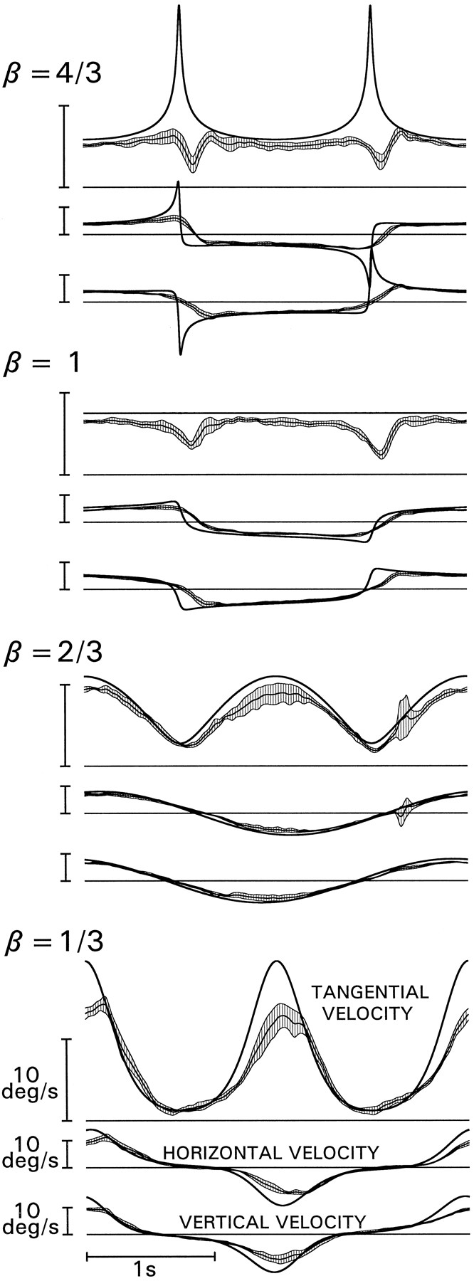
The nature of smooth pursuit failures can be appreciated further by comparing the time course of the tangential velocity for the stimulus and the response (Fig. 5, top traces). The oculomotor kinematic response (averaged over all cycles and all subjects) showed a systematic pattern of deviations from the stimulus. When target tangential velocity increased with the radius of curvature more than prescribed by the Two-Thirds Power Law (β < 2/3), peak eye velocity fell short of target velocity. Moreover, the small lag already present for β = 2/3 became more noticeable. When the target accelerated at the poles (β > 1), the eye actually decelerated. The influence of the geometrical properties of the trajectory is seen most clearly when β = 1, in which kinematic factors should have the least impact. Although in this case the target’s tangential velocity was constant, pursuit velocity was clearly modulated. The velocity components of both stimulus and smooth pursuit (Fig. 5 panels,bottom traces) show that failures are associated with smoothing of acceleration peaks (see below).

Tangential velocity and derivatives of the cartesian components of the smooth pursuit. Averages for all cycles and subjects for the indicated values of β at Σ = 0.968 in the first experimental condition. The 95% confidence bands (shaded areas) were computed from individual means over nine cycles.Thick lines indicate tangential and component velocities of the target. Thin horizontal lines indicate zero reference.
The results presented thus far point to the possibility of accounting for the failures of the pursuit system with a single hypothesis, namely, that irrespective of target kinematics, the smooth component of the response remained constrained by the Two-Thirds Power Law. The hypothesis was confirmed by comparing the R–Vrelation in the data with that prescribed by the targets. First, individual R and V samples for the eye were collapsed into one set of 1500 mean data points covering one complete cycle. Then we pooled all individual sets and performed a normal regression analysis in log–log scales (in logarithmic scales, a power function becomes a straight line with a slope equal to the exponent, which in our case is 1-β). Figure 6 shows the population scatter plots, the associated regressions, and theR–V covariation in the target. As predicted, pursuit velocity was indeed a power function of the radius, and the exponent for the response was largely independent of the exponent for the target. Regressions performed on individual sets of data points confirmed the validity of the power law for each subject (across all conditions and subjects, the normal coefficient of correlation ranged between 0.917 and 0.974). Figure 7 summarizes the comparison between target and pursuit by plotting the averages over all subjects of the β values of the pursuit as a function of the target’s β. Consistent with our hypothesis, the β values for the response were weakly dependent on the kinematics of the stimuli and, for all eccentricities, crossed the required β (dashed line) in correspondence of the Lissajous case (β = 2/3). Thus, irrespective of the target’s exponent, eye velocity modulation remained close to that predicted by the power law for that trajectory.

Relationship between radius of curvature and tangential velocity during smooth pursuit in the first experimental condition. Data points indicate instantaneous values ofR and V in logarithmic scales. Results for the indicated selected β at Σ = 0.968 and all subjects.Thick lines indicate covariation of R andV of the targets. A regression analysis estimated β from the slope of the major axis of the confidence ellipse (thin lines) and the so-called normal coefficient of correlation (Emax −Emin)/(Emax +Emin) (Emax andEmin, larger and smaller eigenvalues of the variance–covariance matrix, respectively). β of the smooth pursuit was only weakly dependent on target’s β.

Smooth pursuit β values (ordinate) as a function of target β values (abscissa). Averages and SD values were calculated from individual regressions. If smooth pursuit reproduced the stimuli faithfully, all data points would fall on the dashed line. This happens only for Lissajous targets (arrow).
Two-dimensional tracking of stimuli compatible with the Two-Thirds Power Law
We suggested above that the main factor responsible for poor pursuit performance with some targets was that they failed to comply with the Two-Thirds Power Law, rather than the large variations of their tangential velocity (in the most critical case, β = 4/3 and Σ = 0.968, the rate of change of the velocity peaked at 360°/sec2). If so, it should be possible to observe a satisfactory performance even with these extreme rates of change, provided the trajectory of the stimulus is modified so as to make it compatible with the Two-Thirds Power Law. The second experimental condition was designed to verify this prediction.
The smooth pursuit velocity for four representative targets is shown in Figure 8, left column, with the same conventions as in Figure 5 (averages computed over all subjects and all cycles). Compared with the results with targets that did not comply with the Two-Thirds Power Law, these traces show a remarkable improvement in pursuit effectiveness. Although smooth pursuit velocity never quite matched that of the stimuli when the rate of change was very high (top-most record), a well-sculptured peak of velocity was always present in these regions. In contrast, when tracking elliptic stimuli with the same velocity functions, pursuit velocity actually decreased in the same regions (compare Fig. 5). Moreover, the systematic lag observed in the first experiment at the lowest values of β was significantly reduced. Also, constant-velocity targets (β = 1) following a circular trajectory did not induce the systematic modulations of the pursuit velocity observed when the motion was elliptic. The improvement in tracking performance was confirmed further by the average number of saccades (Fig. 9, top panel), which was smaller than in the first condition (pooling individual differences between stimuli with the same velocity function,t20 = 5.43, p < .001) and by both mismatch indexes (Fig. 9, middle and bottom panels), which were also significantly smaller (for smooth pursuit, t20 = 6.07, p < .001; for saccades, t20 = 4.35, p < .001; differences were not significant when the comparison was limited to the targets with β = 2/3). As predicted, the limited capacity of the eye to match large variations of tangential velocity can account only marginally for the failures of the pursuit system to cope with targets that violate the Two-Thirds Power Law.

Tracking compatible targets, second experimental condition. Average number of saccades per cycles (top panel) and mismatch indexes (middle andbottom panels) as a function of target type. Results for three subjects are presented in the same format as in Figure 3. Target types are identified by letters referring to the β values for the corresponding targets in the first condition (A, β = 4/3; B, β = 7/6;C, β = 1; D, β = 5/6;E, β = 2/3; F, β = 1/2;G, β = 1/3). For comparison, the dotted lines report again the data in Figure 3 for Σ = 0.968.
One-dimensional tracking of stimulus components
The third experimental condition was designed to investigate the extent to which the properties of 2-D tracking movements can be inferred from the performance with 1-D stimuli. Specifically, we asked whether the R–V covariation described by the Two-Thirds Power Law would emerge by adding vectorially horizontal and vertical tracking responses, each with its own dynamic characteristics. Figure 10 summarizes the performance of the three subjects who tracked the components of the elliptic stimuli used in the first condition. The format is the same as for Figures 5 and 8. In this case, however, the velocity components were measured directly from independent 1-D trials, whereas the tangential velocity was reconstructed by vector addition. Qualitatively, the velocity components are similar to those computed from 2-D pursuit movements (first condition), and so are, by necessity, the reconstructed and 2-D tangential velocities. Thus, the tendency to slow down at the points of high curvature of the trajectory can be predicted qualitatively from the dynamic characteristics of 1-D tracking. However, analysis in the frequency domain revealed significant quantitative differences between 1-D and 2-D performance.

Tracking 1-D targets, third experimental condition. Smooth pursuit velocity while tracking independently the horizontal and vertical components of the targets used in the first experimental condition (Σ = 0.968 for the indicated β). The reconstructed tangential velocity was computed by vector sum of the velocity components. Averages and 95% confidence bands were calculated on three subjects; same format as in Figure 5.
Tracking response characteristics across conditions: a spectral analysis
Comparing the components of smooth pursuit velocity with those of the targets in the time domain (Figs. 5, 8, 10) suggests that in all three conditions, the input–output characteristics of the pursuit system are similar to that of a low-pass filter. However, by analyzing the results in the frequency domain, we found that pursuit behavior depended on the stimuli and could not be interpreted by standard linear system theory. Figure11A–Ddescribes the gain and phase (Bode plots) of the input–output characteristics of the horizontal and vertical components in the first experimental condition. The results are relative to the target with Σ = 0.968 and β = 4/3. They were obtained by averaging the individual Bode plots over all nine subjects. Phase estimates were no longer reliable beyond 6 Hz. Up to ∼5 Hz, the gain could be well approximated by the amplitude function of a four-pole low-pass filter (continuous lines). However, nonlinear spectral components generated by the oculomotor system appeared at higher frequencies, at which the input stimulus did not contain appreciable power. More importantly, even in the low-frequency range, the phase was grossly at variance with the phase function of the filter, suggesting the presence of anticipation in the oculomotor response. Attempts to model the anticipatory component with an exponential term in the transfer function (i.e., by assuming a constant time lead) did not yield a significantly better fit.

Analysis of the smooth pursuit system in the frequency domain. A, B, Gain and phase characteristics (Bode plots) of the smooth pursuit velocity components in the first experimental condition. Results for one target (Σ = 0.968, β = 4/3). Averages and 95% confidence intervals computed from individual Bode plots. For both horizontal and vertical components, the transfer function of a four-pole low-pass filter (continuous lines) fits well the gain data points up to ∼5 Hz. At all frequencies, the same transfer function predicts a much larger phase lag than the data points, suggesting a predictive component in the pursuit system. Beyond 5 Hz, stimuli did not have appreciable power. Harmonic components of the oculomotor response in this range were generated internally. C, D, Comparison in three subjects of the horizontal and vertical gain characteristics between the first and second experimental conditions. First condition, results for one target (Σ = 0.968, β = 4/3, topmost tracesin Fig. 5). Second condition, compatible target with the same tangential velocity distribution (topmost traces in Fig.8). The dynamic range of the system was much wider when pursuing compatible targets than when pursuing targets that violate the Two-Thirds Power Law. E, F, Comparison in three other subjects of the gain characteristics between the first and third experimental conditions. First condition, target as inC and D; second condition, components of the same target but tracked separately. The dynamic response of the pursuit system in the 1-D case was significantly better than in the 2-D case. In all three conditions, responses along the vertical direction were more sluggish than responses along the horizontal direction.
Figure 11, C and D, compares the gain characteristics between the first and second experimental conditions (data averaged over the 3 subjects who served in both conditions; for clarity, nonlinear spectral components are not shown). The gain of the response to targets compatible with the Two-Thirds Power Law was higher than the gain of the response to noncompatible targets. For the horizontal component, the gain drop in the noncompatible condition was significant at the 0.01 level or better for each frequency between 3 and 5.66 Hz (one-tailed t test on paired differences). In this range, the average gain drop was 12.8 dB (for pooled differences,t14 = 11.16, p < .01). For the vertical component, the gain drop was significant at the 0.01 level or better for each frequency between 1 and 5.66 Hz (average gain drop, 15.5 dB; pooling differences, t14 = 20.22,p < 0.01). Thus, spectral analysis confirmed that pursuit performance was stimulus-dependent, being much more effective when the targets followed the power law.
Finally, Figure 11, E and F, compares the gain characteristics between the first and third conditions (data in 3 subjects). The gain of the 1-D pursuit of the components of noncompatible targets was higher than the corresponding gain computed from 2-D trials. For the horizontal component, the difference was significant at the 0.025 level or better for each frequency between 3.66 and 5.66 Hz (average gain drop, 5.9 dB; pooling differences,t14 = 6.17, p < 0.01). For the vertical component, the difference was significant at the 0.01 level or better for each frequency between 3 and 5 Hz (average gain drop, 3.09 dB; pooling differences, t14 = 5.12,p < 0.01). Possibly because of coupling between components, testing the horizontal and vertical systems separately does not permit one to account fully for the performance observed when pursuing noncompatible 2-D targets.
DISCUSSION
By testing the oculomotor tracking behavior with 2-D point targets, we found that smooth pursuit eye movements comply with the same relational constraint (Two-Thirds Power Law) demonstrated in hand movements (Fig. 6). The smooth component of the tracking response was most effective when the stimulus complied with the power law rule, marked degradation of the performance occurring pari passu with the (controlled) extent to which the rule was violated (Figs. 3, 5). Moreover, the distribution of tracking errors (Fig. 4) was strikingly similar to that observed when the hand tracks similar visual (Viviani and Mounoud, 1990, their Fig. 4) and kinaesthetic (Viviani et al., 1997, their Figs. 7, 8, 9, 10) targets. Because of the large anatomical differences between the hand and eye, these behavioral similarities seem to rule out conclusively the hypothesis that the covariation between curvature and velocity reflects specific biomechanical properties of the body segments involved in the task.
The considerable dissociation between the central efferent pathways of hand and eye pursuit systems also limits the number of plausible hypotheses concerning the neural bases for Two-Thirds Power Law. The pontine pathway that conveys smooth pursuit commands to the oculomotor nuclei and, ultimately, to the extraocular muscles, is entirely segregated from the cortico-spinal pathway controlling hand movements. At the cortical level, the amount of segregation is less clear. In fact, both visuo-manual pursuit tracking and smooth pursuit eye movements are controlled by extrastriate visual areas such as middle temporal and medial superior temporal, as well as the parietal area 7a (Lisberger et al., 1987; Jeannerod, 1988; Thier and Erickson, 1993). Recently, it has also been shown that frontal cortical areas are involved in smooth pursuit eye movements (Gottlieb et al., 1994). In addition, both eye and hand control circuitry include the cerebellum, which may perform similar operations in the two cases (Bloedel, 1992). However, a curvature–velocity covariation is also present in hand movements performed without visual control, either extemporaneously or under kinaesthetic guidance (Viviani et al., 1997). Thus, the fact that hand movements share early portions of their controlling pathway with eye movements cannot explain why the law applies in both cases. These arguments lead us to answer the first question addressed here by concluding that the Two-Thirds Power Law should express some general principles of operation common to the distinct modules responsible for setting up the motor output to the hand and the eye.
The comparison between stimulus and response velocity components for some of the targets (e.g., when β = 4/3 and β = 7/6; see Fig. 5) suggests that one such principle be purely kinematic. Specifically, errors may reflect partly the limited capacity of the pursuit system to deal with high linear accelerations, independently of theR–V covariation. However, kinematics alone cannot account for the complete pattern of results. In fact, the fundamental frequency (St. Cyr and Fender, 1969) and velocity (Mayer et al., 1985; Pola and Wyatt, 1991) of the target components were within the working range of the smooth pursuit system, and the response was constrained by the power law, even when the rate of change of the tangential velocity remained within this range (Lisberger et al., 1981). Moreover, although targets contained harmonic components up to ∼5 Hz (see Results), both 1- and 2-D targets remained predictable, as also indicated by the phase characteristics of the responses (Fig.11A,B). Thus, errors should not reflect the well-known difference between pursuit performance with predictable and unpredictable targets (Barnes et al., 1987; Barnes and Asselman, 1991). More importantly, the second experimental condition demonstrated, both in the time (Fig. 8) and in the frequency (Fig. 11) domains, that pursuit performance improved substantially when the same kinematics that proved difficult to deal with in the first condition was coupled with a trajectory that made the target comply with the power law. On the basis of these arguments, we qualify the answer to our main question by arguing that the phenomenon described by the Two-Thirds Power Law does not refer to a purely kinematic limitation, but rather pertains to the covariation between geometry and kinematics of the movement. In what follows, we discuss the second issue raised by the study, namely, the connection between the power law and the modality with which 2-D movements are planned and executed.
If displacements were represented centrally in terms of endpoint coordinates, and their geometrical components were planned independently—as is the case, by analogy, in pen plotters—it should be possible to predict the Two-Thirds Power Law from the kinematics of horizontal and vertical movements. Previous studies (Viviani et al., 1987; Viviani and Mounoud, 1990) showed that such a derivation is not possible for visually guided hand movements. Despite the qualitative similarity between the velocity components derived from 2-D recordings (Fig. 5) and those measured directly (Fig. 10), the comparative analysis in the frequency domain (Fig.11E,F) lead to the same conclusion for oculomotor pursuit (see also Collewijn and Tamminga, 1984). Because movement components are not planned independently, one should ask what kind of direction coding may account for the coupling between components that is responsible for the quantitative aspects of the covariation between curvature and velocity.
Studies on manual reaching and pointing (Bock and Eckmiller, 1986;Bock, 1992; Gordon et al., 1994a,b; Vindras and Viviani, 1997) provide evidence that the motor control system represents target position as a vector in an extrinsic system of coordinates, by specifying extent and direction of the movement for reaching that point. This view is in keeping with the demonstration that neural activity in the motor cortex of primates pointing to (Georgopoulos et al., 1982, 1983, 1988;Schwartz et al., 1988; Caminiti et al., 1990) or tracking (Schwartz, 1992, 1994) visual targets can be interpreted as a distributed vector representation of the intended movement. Moreover, pointing experiments in which the required movement did not coincide with target direction showed, during the latent period, a progressive reorientation of the neural population vector from the visual to the motor direction (Georgopoulos et al., 1989). This may be taken to suggest that the neural events underlying directional coding have their own dynamics: the larger the required change in direction, the longer it takes to rotate the population vector.
Postulating also for the eyes a coding system similar to the one hypothesized for the hand provides a plausible framework for explaining why the Two-Thirds Power Law applies to both hand and eye movements. In fact, developing an early suggestion by Viviani and Terzuolo (1982),Pellizzer et al. (1993) have argued that the relative constancy of the angular velocity of voluntary movements implied by the power law reflects the almost constant rate at which the population vector rotates. In other words, the Two-Thirds Power Law would express a limitation in the rate at which control commands from the motor planning centers can modulate the activity of the neuron pool that collectively codes for the direction of the population vector. If so, the fact that smooth pursuit eye movements comply with the power law would follow from the assumption that such a basic constraint applies to several central modules involved in issuing motor commands. The results in the second experiment are congruent with this hypothesis, because, for each distribution of tangential velocity, compatible targets had lower peaks of angular velocity than those in the first experiment.
APPENDIX
We describe the procedure for specifying form and kinematics of the targets used in the experiments. In the first experimental condition, targets followed elliptic trajectories with a fixed major axis and various values of the eccentricity Σ. LetBx and By, the major and minor semiaxes of the ellipse, respectively (i.e., Σ = (1 − (By/Bx)2))1/2) and let Q be the perimeter. Because Q =Bx4E(π/2, Σ) (E, incomplete elliptic integral of the second kind) andBy = Bx(1 − Σ2)1/2, both Q andBy are determined uniquely byBx and Σ. For any choice ofBx, Σ, and the motion period T, the scalar velocity of the target was selected within a one-parameter family of periodic functions related to the curvature of the trajectory. The procedure was as follows. The general parametric equations of the trajectory are:
 Equation 1Awhere φ(t) is any strictly monotonic, differentiable function of time such that φ(0) = 0 and φ(t) = 2π. By the chain rule for differentiating composite functions:
 Equation 2A(and similar expressions for the ycomponent), one has:
 Equation 3Awhere derivatives with respect to φ are taken at φ = φ(t). Given any non-negative continuous periodic function V(t) with period T, there is a unique function φ(t) satisfying the boundary conditions [φ(0) = 0, φ(t) = 2π] such that the scalar velocity of the motion defined by Equation A1 is V(t). In particular, consider the family of scalar velocity functionsV(t, β) defined by the β-power relation:
 Equation 4Awhere K, β, and α are parameters, andR(t) is the radius of curvature of the trajectory:
 Equation 5AThese velocity functions correspond to the family of Generalized Lissajous Elliptic Movements (GLEMs) introduced by Viviani and Schneider (1991). For this application, we set α = 0. Thus, substituting Equation A1 in Equations A3 and A5, taking into account Equation A4, and solving for dφ/dt yields:
 Equation 6AThis is a separable, nonlinear differential equation of the first order. Inserting the solution φ(t) into the parametric (Eq. A1), one obtains a GLEM, i.e., an elliptic motion that satisfies constraint A4. Notice that for a given trajectory, the law of motions = s(t) of the target is uniquely specified by the parameters β and K becauseds(t)/dt =V(t, β).
For each of the seven selected values of β (see Materials and Methods), Equation A6 was integrated numerically with a standard Runge–Kutta routine. For one complete cycle to be described exactly by 1000 samples (see Materials and Methods), the velocity parameterK and the integration step δτ must be set appropriately. This was performed as follows. Separating the variables, and integrating formally Equation A6, one finds that the analytic solution φ is periodic, and the velocity parameter is related to the period by the equation:
 Equation 7Awhere:
 Equation 8AThus, the condition of periodicity was satisfied by using Equation A7 and setting the integration step to δt =T/M. Notice that T is a computational variable and not the actual period of the targets expressed in seconds. The latter was dictated by the output rate of the digital-to-analog converter.
As for the second experimental condition, consider a point-motion with a GLEM scalar velocity function V(t, β). The problem is to define a trajectory such that, following this trajectory, the motion complies with the Two-Thirds Power Law, i.e., with the special case of Equation A4 that is obtained when β = 2/3. It is known (Guggenheimer, 1963, Theorem 2.13) that a trajectory is uniquely specified, up to a rigid roto-translation, by its radius of curvature at all curvilinear coordinates. Because V(t, β) specifies uniquely the radius of curvature as a function of time (via Equation A4) and the curvilinear coordinate s(t) is a single-valued function of time, the stated problem has a unique solution. Let x = x(t) andy = y(t) be parametric equations of the desired trajectory and:
 Equation 9Athe required velocity. Setting again α = 0, the Two-Thirds Power Law can be written as:
 Equation 10ABy introducing the auxiliary variables z(t) = dx(t)/dt andw(t) = dy(t)/dt, Equations A9 and A10 can be written as a system in the unknowndz(t)/dt anddw(t)/dt:

 which can be separated into two first-order nonlinear differential equations. Solving for dz(t)/dtyields:
 Equation 12AIt can be shown that the horizontal component of a GLEM velocity vanishes at t = 0. Thus, the appropriate boundary condition for Equation A12 is z(0) = 0. By construction, the resulting motion has the same tangential velocity and period as the GLEM that provides its kinematic model. However, because the distribution of the radii along the trajectory is different in the two cases, the parameter K appearing in Equation A12 must be set appropriately to satisfy the condition that the two perimeters be equal. The value of K was found with a standard procedure of successive approximations. The solution z was computed by solving Equation A12 numerically, using again the Runge–Kutta method. Finally, the x component of the trajectory was obtained by integrating z. The other component was computed by substituting x in Equation A9 and solving fory.
Footnotes
This research was supported in part by S. Raffaele Scientific Institute Research Grant #A2876.
Correspondence should be addressed to Prof. Paolo Viviani, Department of Psychobiology, Faculty of Psychology and Educational Sciences, University of Geneva, 9, Route de Drize, 1227 Carouge, Switzerland.


