

Article Figures & Data
Figures
- Figure 1.
Experimental setup. A, Configuration of the experimental apparatus. The subject was instructed to move the hand from the button switch to the center of the display in response to a series of auditory signals. Experiments were performed in a darkened room. B, Time course of the visual stimulus. For details, see Materials and Methods.
- Figure 2.
Temporal patterns of manual response induced by visual motion. A, Mean hand velocity patterns (n = 40) in x-direction in the rightward (R; solid curve) and leftward (L; dashed curve) visual motion (40% contrast, 0.087 c/°, 8.37 Hz). B, Corresponding acceleration patterns. C, Differences between x-directional hand velocity patterns for the rightward and leftward stimuli with image contrast of 2% (thin solid curve), 40% (thick solid curve), and 70% (dashed curve) (0.087 c/°, 8.37 Hz). D, These acceleration patterns. The open, filled, and open-dashed triangles indicate the latencies (152, 124, and 108 ms) detected from MFR acceleration responses in 2, 40, and 70% contrast conditions.
- Figure 3.
MFR amplitude and latency modulation by changing image contrast. Solid and dotted lines show the mean amplitudes and latencies of the MFR, respectively. Amplitude error bars denote the SE for all subjects (n = 6). Each error bar for the mean latency denotes the SE for subjects whose MFR latency was reliably detected (n = 5 for 2 and 10% contrast conditions; n = 6 for other contrast conditions). Spatial and temporal frequencies of the stimulus were 0.087 c/° and 8.37 Hz.
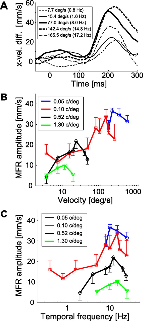
- Figure 4.
Variations of MFR response with changing stimulus image spatiotemporal frequencies. A, Temporal patterns of hand x-velocity of a typical subject for several stimulus velocities. The stimulus velocity and corresponding temporal frequency for each curve are shown in the legend box. Image spatial frequency was 0.10 c/° for all conditions. B, Velocity tuning functions of MFR for four constant spatial frequencies, 0.05, 0.10, 0.52, and 1.30 c/°, averaged over subjects (n = 5). C, Temporal frequency tuning functions of MFR for those stimuli. In B and C, each colored line represents a single spatial frequency condition. Error bars show the SE across subjects (n = 5).
- Figure 5.
Relationship between stimulus velocity and MFR amplitude. Open circles denote the experimental data points for which temporal frequency was lower than 15.1 Hz. The solid line shows a linear regression line of these data, AMFR = 6.17 × log(V) + 0.96, where AMFR and V denote MFR amplitude and stimulus velocity, respectively. The coefficient of determination by the regression was 0.85.
- Figure 6.
Spatiotemporal tuning surfaces of MFR, OFR, and motion perception sensitivity. A, A two-dimensional Gaussian surface fitted to the MFR amplitudes for different spatiotemporal frequencies. Fs, Spatial frequency; Ft, temporal frequency. The color indicates the height (MFR amplitude) of the surface normalized by maximum and minimum values in the overall data: dark red, highest; dark blue, lowest. Magenta circles are the data points obtained in the experiment. The VAF was 0.84. The black curves superimposed on the fitted surface represent the data points for the constant stimulus velocities of 4, 10, 20, 60, 100, and 160 °/s. B, Top view of the fitted surface (color contour plot). MFR amplitude along any constant spatial frequency (ordinate) increases as spatial frequency decreases. MFR amplitude increases with temporal frequency until ∼15–20 Hz but decreases thereafter. This trend was also observed in the experimental data in Figure 4C. Small black dots denote the data point on the surface corresponding to the experimental data. C, Color contour plot of the tuning surface of the OFR amplitudes, fitted to the data of Miles et al. (1986). The VAF value was 0.91. D, Color contour plot of the tuning surface of the perceptual contrast sensitivity of visual motion. The VAF value was 0.99. For description of the basis functions fitted to the data, see Materials and Methods. The peak of the sensitivity-tuning surface is clearly different from those of the MFR (B) and OFR (C). In B–D, color indicates the height of the fitted surface normalized by maximum and minimum values in each region: dark red, highest; dark blue, lowest.


