

Article Figures & Data
Figures
- Figure 1.
Transfer functions with expansive nonlinearities lead to right-skewed rate distributions. A, Given a Gaussian distribution in inputs across neurons, a linear transfer function ϕ, where ν = ϕ(I), will result in a Gaussian population firing rate distribution. B, If ϕ exhibits an expansive nonlinearity, then the Gaussian input distribution will be skewed such that the peak is pushed toward low firing rates and a long tail is formed at high firing rates. The function ϕ here is exponential, which results in a lognormal firing rate distribution.
- Figure 2.
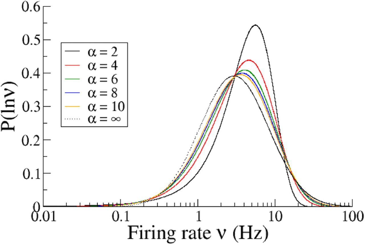
Distribution of the logarithm of the firing rate for power-law transfer functions with different powers. The mean μ̄ and variance Δ2 of the Gaussian input distribution were adjusted to fix the mean at 5 Hz and the variance of the logarithm of the rate at 1.04. As α is increased, the distribution of the logarithm of the rate approaches a Gaussian distribution, indicating that rate distribution more closely approaches a lognormal distribution (indicated for comparison with a dotted line).
- Figure 3.
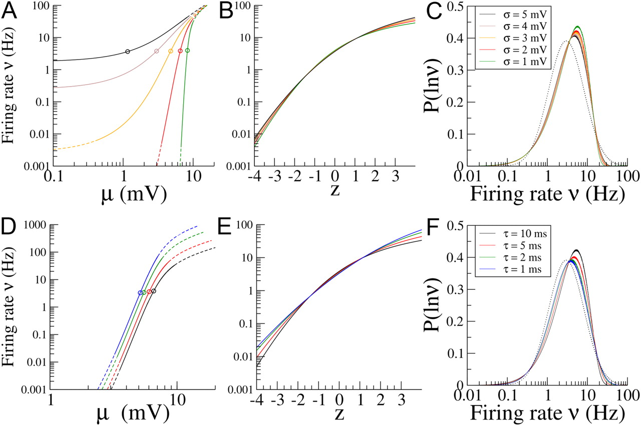
Transfer function and firing rate distribution for a population of integrate-and-fire neurons. A, Log–log plot of the firing rate, ν, versus the input, μ, for different values of the noise intensity σ (indicated in C) and with τ = 10 ms. The firing rate approaches a constant value as μ → 0. It increases with σ. On a log–log plot, there is a region for intermediate firing rates in which the f–I curve is approximately a straight line. This corresponds to a power-law f–I relationship with an exponent that increases for decreasing σ. The mean of the input distribution is indicated by an open circle, and the solid portion of each line spans 4 SDs of the input distribution. B, Firing rate as a function of the normalized input z = (μ − μ̄)/Δ on a semi-log plot in which a straight line indicates an exponential dependency. C, Distribution of ln(ν) for different values of σ. The mean and variance of the input was adjusted so that, for all values of σ, the mean firing rate was 5 Hz, and the variance of the logarithm of the firing rates was 1.04. The dotted curve is a lognormal distribution with the same mean and variance. D–F, Same as for A–C but for a fixed value of σ = 2 mV with τ = 10, 5, 2, 1 ms.
- Figure 4.
The distribution of firing rates for a network of uncoupled LIF neurons (Eq. 38) for different values of the population-averaged mean firing rate. Here the mean firing rate averaged over the population increases, while the variance of the log of the rates is held fixed at 1.04. Parameters: τm = 2 ms; μ̄ = 4.73, 5.89, 6.37 mV; Δ2 = 0.187, 0.28, 0.36, 0.5 mV2; σ = 2 mV, lead to v̄ = 1, 5, 10, 20 Hz, respectively.
- Figure 5.
Firing rate distributions in randomly connected networks of LIF neurons in an asynchronous irregular state. A, The distribution of mean inputs across neurons in the LIF network. The solid line was generated numerically from a run of 10 s, and the dashed line is a Gaussian function, the mean and variance of which are given by Equations 15 and 16, respectively. The inset shows the distributions of excitatory (exc) and inhibitory (inh) connections (with means 1000 and 250 subtracted off, respectively), which are also close to Gaussian. B, The top panel shows a raster diagram of the activity of 30 randomly chosen neurons from the simulation. The bottom panel is the membrane voltage of one neuron. Both the spiking and subthreshold activities are irregular. C, The numerically determined firing rate distributions from a simulation lasting 10 s. The mean of the distribution is indicated by the white arrow, and the median is indicated by the black arrow. D, The distribution of the logarithm of the firing rate. Results from the simulation are shown as filled symbols in which the error bars show the SD over 10 runs of 10 s each. The solid line is the best-fit lognormal distribution. Note that there is an excess of neurons firing at low rates and a dearth of neurons firing at high rates in the simulation compared with the lognormal fit. Parameter values: τE = τI = 20 ms; NE = 10,000; NI = 2500; p = 0.1, θ = 20 mV; Vr = 10 mV; JEE = JIE = JextE = JextI = 0.2 mV; JII = J EI = −1.2 mV; CextE = CextI = 1000; νextE = νextI = 5.5 Hz.
- Figure 6.
Distribution of firing rates for a network of two populations in which excitatory and inhibitory neurons fire at different mean rates. Shown are three firing rate distributions calculated analytically from Equation 22. The blue one shows the case of identical firing rates in both populations of neurons. The red, black, and orange curves show how the distribution changes as the inhibitory cells fire at increasingly higher rates. The clearest effect is the broadening of the tail at high rates. In all cases, the mean and SD of the log rates have been fixed. The dotted curve is a lognormal distribution with the same mean and SD. Parameters: νextE = 23, 30.35, 32.9, 47.05 Hz; νextI = 23, 32.55, 35.95, 50.68 Hz; ΔC2 = 2000, 620, 50, 0; JEE = JIE = JextE = JextI = 0.0713, 0.0713, 0.0713, 0.048 mV; JII = JEI = −6JEE mV for the blue, red, black, and orange curves, respectively. The remaining parameters are the same: τE = τI = 5 ms; CextE = CextI = 1000.
- Figure 7.
Comparison of results from LIF network and experimental data. Distributions of the logarithm of the firing rate. A, Black, From 10 simulations, each with a different realization of network connectivity, of 10 s duration each; error bars indicate 2 SDs. Red, From spontaneously active neurons in auditory cortex; error bars indicate 95% confidence intervals. Solid line, Analytically determined distribution from Equation 22. Parameters for the simulations: τE = 5 ms; τI = 2.5 ms; NE = 8000; NI = 2000; p = 0.125; θ = 10 mV; Vr = 0 mV; JEE = JextE = 0.188935 mV; JIE = JextI = 1.75 JEE mV; JEI = −3.5 JEE mV; JII = −3.5J IE mV; CextE = CextI = 1000; ΔC2 = 2000; νextE = 10.29 Hz; νextI = 9.99 Hz. There is a uniform distribution in synaptic delays from 0.1 to 3.1 ms. B, Black circles, From barrel cortex of awake mice. Solid line, Analytically determined distribution from a network of uncoupled LIF neurons (Eq. 22) with μ = 4.85 mV, σ = 2.2 mV and Δ =
 mV. Dashed line, Best fit to a lognormal distribution.
 - Figure 8.
Firing rate distributions in a network of conductance-based neurons in the fluctuation-driven regimen. Parameters are given in Material and Methods. A, Sample traces from three excitatory neurons. B, Sample traces from three inhibitory neurons. C, The distributions of CVs of excitatory neurons (black line) and inhibitory neurons (red line). D, The firing rate distributions, for several values of σg, indicated on the figure. Symbols are from simulations, and lines are best-fit lognormals. Parameters are given in Material and Methods. In A–C, σg = 0.


