

Article Figures & Data
Figures
- Figure 1.
Dentate hilar cell death and increased excitability after concussive brain injury. A, Representative Fluoro-Jade C-stained section from a rat perfused 4 h after sham injury shows no fluorescently labeled neurons, illustrating the absence of dying neurons in sham-injured controls. B, Fluoro-Jade C-stained section from a rat perfused 4 h after FPI shows numerous labeled dying neurons in the hilus. C, Representative traces of granule cell layer field responses evoked by perforant path stimulation in slices from a sham-injured (left) and head-injured (right) rat obtained 1 week after FPI illustrates the larger population spike amplitude in the injured dentate gyrus compared with sham injury. Traces are an average of four trials in response to a 4 mA stimulus to the perforant path. Arrows indicate location of stimulus artifact that was truncated. D, Summary data demonstrate the postinjury increase in afferent-evoked excitability of the dentate gyrus at various stimulation intensities. Error bars indicate SEM. *p < 0.05, unpaired Student's t test. Wk, Week; GCL, granule cell layer.
- Figure 2.
Features that distinguish granule cells from semilunar granule cells. A, Illustration of a fully reconstructed granule cell shows the typical location of the somata in the granule cell layer (GCL) and compact dendritic spread in the molecular layer (ML). The axon (mossy fiber, thin line) is seen projecting in the hilus, toward CA3. Inset, Confocal image shows labeling for biocytin (left), Prox1 (middle), and the merged image (right), illustrating colabeling. Scale bar, 5 μm. B, Reconstruction of a biocytin-filled semilunar granule cell shows the location of somata in the ML and demonstrates the wider dendritic span compared with the granule cell in A. Note the high degree of branching of the SGC axon (thin line) in the hilus and projection to CA3. Inset, Confocal image of the somata of the SGC in B shows labeling for biocytin (left), Prox1 (middle), and the merged image (right), illustrating colabeling. Scale bar, 5 μm. C, Membrane voltage traces from the granule cell in A show the highly adapting firing pattern in response to +200 pA current injection and hyperpolarization during a −120 pA current injection. D, Current-clamp recordings from the semilunar granule cell in B illustrate the continuous firing with low adaptation during a +200 pA depolarizing current injection from a holding potential of −70 mV. Note that the hyperpolarization in response to a −120 pA current injection is smaller than in the granule cell in C. Inset, Expanded membrane voltage trace shows the slow ramp depolarization (arrowhead) and large, slow afterhyperpolarization (arrow) that are distinctive of SGCs. E, Summary histogram shows lower spike frequency adaptation ratio (i.e., higher adaptation) in granule cells compared with SGCs. F, Summary plot illustrates the low input resistance of SGCs compared with granule cells. *p < 0.05, Student's t test.
- Figure 3.
Increase in excitability of semilunar granule cells after brain injury. A, B, Biocytin-filled and reconstructed semilunar granule cells in experiments performed 1 week after sham injury (A) and head injury (B) show the SGC soma in the molecular layer (ML) and widespread dendrites (thick lines). Axons (thin lines) of both control and injured SGCs are seen projecting toward CA3. Note the axon collateral in the inner molecular layer (arrowhead) of the control SGC in A. Insets, Confocal images of biocytin (left) and Prox1 labeling (middle) of the SGC soma. The merged images (right) demonstrate Prox1 labeling in SGCs from both sham-injured and FPI rats. Scale bar, 5 μm. C, Example membrane voltage traces from the sham-injured SGC in A show the nonadapting firing in response to a +200 pA current injection and hyperpolarization during a −120 pA current injection. D, Representative recordings in the FPI SGC in B illustrate the higher firing frequency for the same +200 pA depolarizing current injection as in C. Additionally, the hyperpolarization in response to a −120 pA current injection is larger than in the sham-injured SGC (C). Note that the characteristic slow ramp depolarization (arrowhead) and large slow afterhyperpolarization (arrow) are observed in the FPI SGC. E, Summary plot of firing rates of sham-injured and FPI SGCs during 1 s depolarizing current steps shows the enhanced firing frequency in FPI SGC. F, Histograms show that FPI SGCs have higher input resistance than controls. Sham-injured SGC data are derived from the same group of cells as in Figure 2. *p < 0.05, Student's t test. GCL, Granule cell layer; Wk, week.
- Figure 4.
Decrease in SGC spontaneous IPSC frequency after FPI. A, Representative traces of voltage-clamp recordings from sham-injured SGCs (top two traces) and FPI SGCs (bottom two traces) show the higher sIPSC frequency in sham-injured SGC (top trace) and the complete block of synaptic events in BMI (100 μm) in the same cell. Note the decrease sIPSC frequency in the recording from an FPI SGC (bottom trace) and subsequent block of synaptic events in BMI (100 μm). B–D, Cumulative probability plots of interevent interval (B), amplitude (C), and weighted decay time constant (D) of sIPSCs recorded in kynurenic acid (3 mm) in sham-injured SGCs (black) and FPI SGCs (gray). Labels in C apply to B and D as well. Vertical dashed lines indicate median of the distribution at p = 0.5. D, Inset, Overlay of normalized average sIPSC traces from a sham-injured SGC (black) and an FPI SGC (gray) illustrate the more rapid decay of sIPSCs after brain injury. The same number of individual events was selected from each cell to develop the cumulative distribution (sham injured: n = 6 cells; FPI: n = 6 cells).
- Figure 5.
Increase in granule cell sIPSC frequency and amplitude after brain injury. A, Example current traces of individual sIPSCs in sham-injured (top two traces) and FPI (bottom two traces) granule cells illustrate the lower frequency and amplitude in sham-injured granule cells compared with FPI granule cells. The block of synaptic events in BMI (100 μm) is illustrated in the respective lower traces. B, C, Cumulative probability plots of granule cell sIPSC interevent interval (B) and amplitude (C) in sham-injured SGCs (black) and FPI SGCs (gray). Vertical dashed lines indicate median of the distribution at p = 0.5. Identical number of events from each cell were used in the analysis (control: n = 12 cells; FPI: n = 7 cells). Recordings were performed in 3 mm kynurenic acid.
- Figure 6.
Decrease in spontaneous and miniature IPSC frequency in SGCs after FPI. A, Representative traces of voltage-clamp recordings from SGCs held at 0 mV show the higher sIPSC frequency in sham-injured SGC (top) and a decrease in sIPSC frequency in the recording from an FPI SGC (bottom). B, Cumulative probability plots of sIPSC interevent interval in sham-injured (black) and FPI (gray) SGCs. Vertical dashed lines indicate median of the distribution at p = 0.5. C, Voltage-clamp recording of miniature IPSCs in sham-injured SGC (top) and FPI SGC (bottom). D, Cumulative probability plots of mIPSC interevent interval in sham-injured (black) and FPI SGCs (gray). Vertical dashed lines indicate median of the distribution at p = 0.5.
- Figure 7.
Intrinsic diversity in SGC and granule cell synaptic inhibition. A, Representative voltage-clamp recordings (Vhold = −70 mV) of individual sIPSCs in a granule cell (top) and an SGC (bottom) from a sham-injured rat. Note the lower sIPSC frequency in the granule cell compared with the SGC. B, Cumulative probability plots compare the sIPSC interevent interval granule cells (black) and SGCs (gray) in control rats recorded in 3 mm kynurenic acid. Inset, Summary histogram of sIPSC frequency in granule cells (GCs) and SGCs. C, Summary histogram of the 20–80% rise time in control granule cells and SGCs. D, Cumulative probability plots of sIPSC amplitude in granule cells (black) and SGCs (gray). Vertical dashed lines indicate median of the distribution at p = 0.5. Identical number of events from each cell were used in the analysis (GC: n = 12 cells; SGC: n = 6 cells). Labels in D apply to B and D. sIPSC data were derived from the same control group of cells as in Figures 4 and 5. *p < 0.05, Student's t test.
- Figure 8.
Decrease in SGC tonic GABA currents after brain injury. A, Representative voltage-clamp recordings (Vhold = −70 mV) from a sham-injured (top) and FPI SGC (bottom) 1 week after injury illustrate the magnitude of tonic GABA current blocked by a saturating concentration of BMI (100 μm). Right, Gaussian fits to all-points histograms derived from 30 s recording periods in control conditions in the presence of 3 mm kynurenic acid, after the addition of THIP (1 μm) and during BMI perfusion used to determine tonic current amplitude. The dashed lines indicate the Gaussian means and the difference currents are noted. B, Summary histogram of the tonic GABA currents in sham-injured and FPI SGC in kynurenic acid. C, Histogram of tonic GABA currents in control aCSF with KyA and following addition of THIP in recordings from both sham-injured and FPI SGCs. D, Summary data of tonic GABA current amplitude measured in THDOC (20 nm) in sham-injured and FPI SGCs. E, F, Cumulative probability plots comparing the sIPSC-weighted decay time constants in aCSF with KyA (black) and following the addition of THIP (gray) in recordings from sham-injured (E) and FPI (F) SGCs. Vertical dashed lines indicate median of the distribution at p = 0.5. Insets, Overlay of normalized average sIPSC traces from a sham-injured SGC (E, inset) and an FPI SGC (F, inset) during recordings in aCSF with KyA (black) and from the same cell following the addition of THIP (gray). The same number of individual events were selected from each cell to develop the cumulative distribution (sham injured: n = 3 cells; FPI: n = 4 cells). *p < 0.05, paired and unpaired Student's t test.
- Figure 9.
Postinjury decrease in SGC tonic GABA currents is maintained in the presence of GABA transporter blocker. A, Representative voltage-clamp recordings (Vhold = 0 mV) from a sham-injured (top) and FPI SGC (bottom) 1 week after injury illustrate the magnitude of tonic GABA current blocked by SR95531 (gabazine, 10 μm). Right, Gaussian fits to all-points histograms derived from 30 s recording periods in aCSF after addition of NO-711 (10 μm) and during SR95531 perfusion used to determine tonic current amplitude. The dashed lines indicate the Gaussian means and the difference currents are noted. B, Summary histogram of SGC tonic GABA currents in aCSF and after addition of NO-711 in recordings from both sham-injured and FPI SGCs. *p < 0.05, paired and unpaired Student's t test.
- Figure 10.
Granule cell tonic GABA currents are increased after brain injury. A, Example voltage-clamp recordings (Vhold = −70 mV) from granule cells from a sham-injured (top) and FPI (bottom) rat obtained 1 week after injury show the presence of tonic GABA current blocked by a saturating concentration of BMI (100 μm). Right, Gaussian fits to all-points histograms derived from 30 s recording periods in KyA after adding THIP (1 μm) and during BMI perfusion. The dashed lines indicate the Gaussian means and the difference currents are noted. Note the larger amplitude of tonic GABA currents in FPI granule cells. B, Summary plot of tonic GABA currents in sham-injured and FPI-granule cells in KyA. C, Histogram of tonic GABA currents in control aCSF with KyA and following addition of THIP in recordings from both sham-injured and FPI granule cells. D, Comparison of tonic GABA current amplitudes between granule cells (GCs) and SGCs in sham-injured and FPI rats. Histograms are based on tonic GABA currents recorded in KyA from the same group of cells as in Figures 8 and 10, A and B. *p < 0.05, paired and unpaired Student's t test.
- Figure 11.
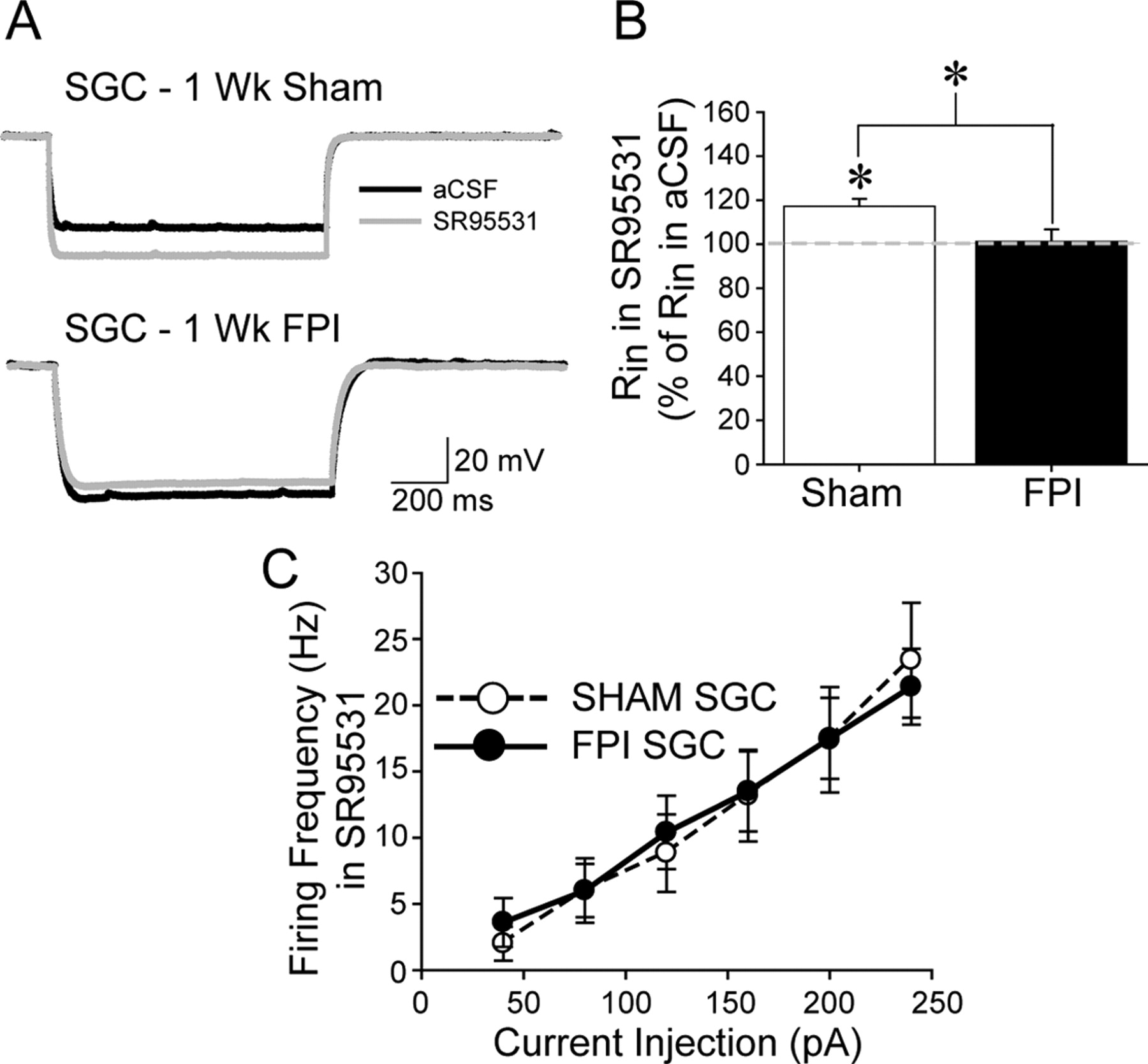
GABAA receptor antagonists enhance SGC input resistance in sham-injured controls but not after FPI. A, Membrane voltage responses to a −120 pA current injection recorded in a control and an FPI SGC illustrate that SR95531 (20 μm) increased the hyperpolarizing response in sham-injured SGCs (top) but failed to alter the response of FPI SGCs (bottom). B, Summary plot of the effect of SR95531 on SGC Rin, expressed as a percentage of Rin in control aCSF, shows that SR95531 enhanced Rin control SGC but failed to alter Rin in FPI SGC. C, Plot of SGC firing rates recorded in the presence of SR95531 (20 μm) reveals the action potential frequency during 1 s depolarizing current steps was not different in sham-injured and FPI SGCs. *p < 0.05 paired and unpaired Student's t test. Wk, Week.


