

Abstract
Motion detection is a fundamental property of the visual system. The gold standard for studying and understanding this function is the motion energy model. This computational tool relies on spatiotemporally selective filters that capture the change in spatial position over time afforded by moving objects. Although the filters are defined in space–time, their human counterparts have never been studied in their native spatiotemporal space but rather in the corresponding frequency domain. When this frequency description is back-projected to spatiotemporal description, not all characteristics of the underlying process are retained, leaving open the possibility that important properties of human motion detection may have remained unexplored. We derived descriptors of motion detectors in native space–time, and discovered a large unexpected dynamic structure involving a >2× change in detector amplitude over the first ∼100 ms. This property is not predicted by the energy model, generalizes across the visual field, and is robust to adaptation; however, it is silenced by surround inhibition and is contrast dependent. We account for all results by extending the motion energy model to incorporate a small network that supports feedforward spread of activation along the motion trajectory via a simple gain-control circuit.
- delayed feedback
- extrapolation mechanism
- gain control
- kernel estimation
- noise image classification
- sequential recruitment
Introduction
Some creatures do not see form or color, but all see motion; it appears that any visual system of reasonable complexity supports motion detection (Nakayama, 1985). Because of its fundamental importance, this property has been studied extensively over the past 60 years at all levels of processing in the visual system of both vertebrates and invertebrates (Borst and Euler, 2011). The earliest breakthrough in this direction came from work in the beetle, which led to the formulation of the Reichardt detector (Reichardt, 1961). The main principles of the Reichardt detector were then found to extend well beyond the visual system of insects and played a paramount role in the understanding of motion processing by vertebrate systems (Clifford and Ibbotson, 2002).
The notion of spatiotemporally oriented filters was introduced and formalized in the 1980s (Burr and Ross, 1986). Although this concept is in many respects equivalent to Reichardt motion detection (van Santen and Sperling, 1985), its formulation in terms of space–time orientation was pivotal in refocusing psychophysical research into human vision (Braddick, 1986). The associated motion energy model (Adelson and Bergen, 1985) quickly became the most powerful tool for interpreting results from a wide range of experimental manipulations, and within a decade established itself as the gold standard for describing human motion detection (Heeger and Simoncelli, 1993). The undeniable success of this model indicated that the general problem of motion detection had been largely solved, prompting investigations into aspects of motion processing beyond detection (Watanabe, 1998).
An oriented filter in space–time corresponds to a localized region of spatiotemporal frequency (Watson and Ahumada, 1983; Simoncelli, 2003). For technical reasons, and in line with the Fourier-based trend that had been dominant since the 1970s (Maffei and Fiorentini, 1973), the frequency description was more readily accessible to investigation, with the result that human motion detection was primarily characterized via estimates of the power spectrum (Burr and Ross, 1986; Clifford and Ibbotson, 2002; for examples of different approaches, see Fahle and Poggio, 1981; McKee and Welch, 1985). These estimates could then be exploited to infer some properties of the underlying spatiotemporal filter, such as tilt and spatial scale (Burr et al., 1986; Anderson and Burr, 1989) without explicitly measuring the filter across the dimensions of space and time. The introduction of reverse correlation techniques into physiological research prompted measurements of the latter kind in single neurons (Emerson et al., 1987), which broadly confirmed at least coarse correspondence between descriptions in space–time (Pack et al., 2006) and those in the frequency domain (Priebe et al., 2006). Such measurements from cells do not find a counterpart in human vision, possibly due to limitations/complications associated with psychophysical variants of reverse correlation (Neri, 2010). The goal of this study was to rectify this lack of evidence by deriving explicit space–time descriptors for human motion detection.
Materials and Methods
Observers and data mass.
We tested 15 naive observers (one male) and the author (P.N.). Naive observers were paid £7/h for data collection. Different subsets of the 16 observers took part in different experiments with differing degrees of overlap. Eight observers took part in the peripheral experiments with both unoriented/oriented noise probes (see Fig. 2B–G) and in the low contrast/second-order experiments (Fig. 8). Seven observers took part in all remaining experiments. The non-naive observer (author) only took part in the peripheral experiments with unoriented probe (see Fig. 2D, open symbol). We collected a total of ∼400,000 trials (average of ∼6000 trials per observer per experiment). Two observers from this pool and four additional observers took part in the experiments with random-dot stimuli (see Fig. 9), for which we collected a total of 7400 trials (average of ∼1200 trials per observer).
Main stimulus.
The motion signal consisted of a bar (80 × 9 arcmin) moving vertically (up or down) over nine frames (each frame lasting 10 ms, corresponding to a speed of ∼15°/s). The bar was dark for experiments involving surround inhibition (see Fig. 4) and adaptation (see Fig. 5); it was otherwise bright. We adjusted signal bar intensity individually for each observer and each experiment to target threshold performance following preliminary testing with a two-down one up staircase procedure. Across observers and experiments, average signal luminance was set to ±7 cd/m2 (+, for bright; −, for dark) around a background luminance of 30 cd/m2; associated performance was 74% correct (SD across entire dataset, 5%). Because the stimulus did not vary across the horizontal dimension, its effective dimensionality is two (space and time); it can therefore be represented in the form of a diagonal line spanning a square spatiotemporal region (Fig. 1A; Adelson and Bergen, 1985). Experiments with square (unoriented) noise probes involved random Gaussian modulations of luminance (SD of 3 cd/m2) independently applied to each spatiotemporal location within the square space–time region; in actual stimulus space, this manipulation consisted of bar-like noise (Neri and Heeger, 2002; Megna et al., 2012; Fig. 1A). Oriented probes involved similar modulations, but aligned with the diagonal space–time direction (Fig. 2E, tilted region).
Presentation protocols and tasks.
We adopted two separate presentation protocols (in different experiments): peripheral two-alternative forced choice (2AFC) and foveal single-presentation binary response. In the former, the upward-moving “target” signal (embedded in noise) was presented to one side of fixation (5° eccentricity), while the downward-moving “antitarget” signal was simultaneously presented to the opposite side of fixation (Fig. 2A). Observers were asked to press Button 1 to indicate that the target signal appeared on the left while the antitarget signal appeared on the right, and Button 2 to indicate that the complementary configuration was presented. In the foveal protocol, only one signal (either target or antitarget) was presented at fixation (Fig. 2H), and observers were asked to press Button 1 to indicate target, or Button 2 to indicate antitarget. Their response was followed by trial-by-trial feedback (correct/incorrect) and initiated the next trial after a random delay uniformly distributed between 200 and 400 ms, except for adaptation experiments (see Fig. 5), during which stimuli were presented at 1 s intervals regardless of whether observers responded or not (if observers responded within the 1 s time window, feedback was delivered and their choice was recorded; if they failed to respond, feedback was not delivered and that trial was excluded from analysis). At the end of each block (100 trials) observers were provided with a summary of their overall performance (percentage of correct responses on the last block as well as across all blocks).
Stimulus variants (low contrast, surround inhibition, adaptation, second order).
Low-contrast experiments (see Fig. 8A–D) conformed to the foveal protocol; stimuli were obtained by reducing contrast (both signal and noise) by a 5× factor (background luminance remained unaffected). The experiments on surround inhibition (see Fig. 4) conformed to the peripheral protocol and involved two high-contrast (100%) gratings (80 arcmin wide; 2.3° high; 0.86 cycles/°; speed, 15°/s) presented immediately to the left and right of each probe (see Fig. 4A,E,I,M, icons). The experiments on adaptation (see Fig. 5) also conformed to the peripheral protocol; the same high-contrast grating (but 100 arcmin wide to ensure that the entire retinotopic region corresponding to the probe would be adapted despite potential eye movements) was presented once at the beginning of each 100-trial block, and then every five trials (four probe trials, one top-up). During blocks of prolonged adaptation, the first presentation of the high-contrast grating (adaptor) lasted 60 s, and subsequent presentations (top-up) lasted 6 s (see Fig. 5I,M). During blocks of brief adaptation, all presentations of the adaptor lasted 90 ms (see Fig. 5A,E). Prolonged and brief adaptation blocks were run separately in different sessions (they were never mixed within the same session, and different sessions were run on different days). Second-order experiments (see Fig. 8E–H) conformed to the foveal protocol, and stimuli were generated by modulating contrast of a binary texture consisting of 3 arcmin dark/bright pixels (0/60 cd/m2). The binary texture (80 arcmin wide, 2.5° high) remained unchanged throughout stimulus presentation and was modulated in bar-like fashion (see Fig. 8E), the size of each bar matching bar size for first-order experiments. Baseline contrast applied to the texture was 50%; signal and noise modulations involved positive/negative excursions around this baseline level. The signal contrast modulation was 16% above baseline. Noise modulations were Gaussian with SD of 6%.
Random-dot experiments.
A square static background texture (measuring 2.6°) consisting of random bright/dark polarity Gaussian dots (5 arcmin SD, density 19 dots/deg2) was presented at fixation and remained the same throughout a given block. During stimulus presentation, dots within a central circular region (1.8° diameter) were animated independently within two consecutive temporal segments. In the “inducer” segment, all dots moved upwards for 80 ms at a speed of ∼15°/s (same speed used with bar stimuli). In the 40 ms “test” segment, a percentage of the dots moved upwards while the remaining dots moved ±22.5° to the left or to the right of vertical. At the end of each trial, observers were asked to indicate whether motion was biased to the left or to the right by pressing one of two buttons. Trial-by-trial feedback was provided, as well as a performance summary at the end of each block (see above). Performance was measured for five logarithmically spaced values of signal percentage (0.0625, 0.125, 0.25, 0.5, 1; see Fig. 9D, x-axis) by the method of constant stimuli. Different values were randomly mixed within each block, as was the order of the two segments: test-followed-by-inducer on “early-test” trials (see Fig. 9B); inducer-followed-by-test on “late-test” trials (see Fig. 9C). Blocks alternated between high-contrast (100%) and low-contrast (20%) stimuli (we collected an equal number of trials for each condition).
Derivation of spatiotemporal perceptual filters.
Each noise sample is denoted by matrix Ni[q,z](x,t): the spatiotemporal (x,t) sample added to target (q = 1) or antitarget (q = 0) signal on trial i to which the observer responded correctly (z = 1) or incorrectly (z = 0). The four panels in Figure 1B–E refer to the four possible ways of classifying a given noise sample: q = 1 and z = 1 (B), q = 1 and z = 0 (C), q = 0 and z = 1 (D), q = 0 and z = 0 (E). The standard formula for combining averages from the four classes into a perceptual filter is P = 〈N[1,1]〉 − 〈N[1,0]〉 − 〈N[0,1]〉 + 〈N[0,0]〉, where 〈〉 is average across trials of the indexed type (Murray, 2011). This rule is applicable when the sensory process operates like a linear matched filter, but not necessarily otherwise (Neri, 2010); in previous work (Neri, 2011), we have demonstrated that under some conditions it becomes manifestly inadequate, and that it must therefore be modified to produce sensible results. For the specific application of interest, it was necessary to modify this rule as follows: P = 〈N[1,1](x,t)〉 − 〈N[1,0](x,t)〉 + 〈N[0,1](−x,t)〉 − 〈N[0,0](−x,t)〉. This modification was motivated by inspection of aggregate data (Fig. 1B–E,J–M) and by relevant computational modeling (Fig. 1F–I). Close inspection of 〈N[1,1]〉 in Figure 1B, which is the 2AFC equivalent of a “hit” classified image (Green and Swets, 1966), demonstrates that (as expected) it resembles the target signal: it modulates along the / diagonal (Fig. 1B, marginal yellow trace), but not along the \ diagonal (Fig. 1B, white trace). Similarly, 〈N[1,0]〉 in C, the equivalent of a “miss” image, conforms to the expectation of an inverted image of the target signal. For both Figure 1B,C the standard rule of adding the former and subtracting the latter is therefore applicable. The standard rule, however, was primarily formulated for designs in which the nontarget is a scaled image of the target (Ahumada, 2002; Murray, 2011). The nontarget we used in this study was an antitarget signal oriented orthogonal to the target, a difference that cannot be accommodated by scaling (with or without sign inversion). For this reason 〈N[0,0]〉 in Figure 1E, the equivalent of a “false alarm” image, is not a scaled version of Figure 1B as is normally expected (Ahumada, 2002) but retains the spatiotemporal orientation of the nontarget signal that was embedded within this noise probe; it is therefore better thought of as a “miss” image where it is the antitarget (rather than the target) that was missed. When viewed this way, it becomes clear why it was necessary to realign its orientation to the target via mirror inversion of the spatial axis (−x rather than x in formula above; Fig. 1I, ↕) before combining it with B and C. A similar procedure was necessary for 〈N[0,1]〉 in Figure 1D, the equivalent of a “correct rejection” image but more appropriately viewed as a “hit” image for the antitarget: because the corresponding noise probes contained an antitarget signal, the signal-related modulation is only present along the \ diagonal (white marginal trace) and not the / diagonal (yellow trace), requiring inversion across the spatial dimension (Fig. 1H, ↕). Following these simple transformations (Fig. 1F–I, orange symbols), the four images in Figure 1B–E are realigned to the same reference (target signal) and can then be combined into a final perceptual filter image (Fig. 2B) that shows a clear structure resembling the target moving bar. It may be argued that orientation realignment may be equally obtained by mirror inverting across the time axis (⇆) as opposed to the space axis (↕). Time, however, is not a symmetric dimension, while space can be regarded as symmetric for the present application. Orientation realignment via mirror inversion across space is therefore the only applicable option. For the analysis involving differential inspection of target and antitarget perceptual filters (see Figs. 4, 5), we computed respectively P[1] = −〈N[1,1]〉 + 〈N[1,0]〉 and P[0] = 〈N[0,0]〉 − 〈N[0,1]〉.
Motion energy model.
Sj (x,t) is the spatiotemporal stimulus presented on interval j. It is initially convolved with “antineutron” front-end filter F[0] and squared to yield Rj[0] = (F[0] * Sj)2; Rj[0] is then subtracted from the corresponding squared convolution with “neuron” filter F[1], i.e., Rj[1] = (F[1] * Sj)2, to obtain Rj− = Rj[1] − Rj[0]; Rj− is integrated across both space and time via weighting function W to obtain final output rj = Σx,t W (x,t)Rj−(x,t). The model selected interval 1 if r1 > r2, interval 2 otherwise; for the purpose of simulating one-interval foveal protocols (when only one stimulus was presented on each trial) the model selected target when r > 0, antitarget otherwise. The shapes chosen for W, F[0], and F[1] in specific simulations are plotted in the relevant figures.
Delayed gain-control model.
Define Rj+ = Rj[1] + Rj[0]. Convolution with the stimulus is recursively updated over time via rule Rj[q](x,t)←Rj[q](x,t) × (Rj+(x,t − τ) + k) where τ = 10 ms (one stimulus frame) and baseline k was set to a fixed value ∼10× the average output of Rj+ across simulations without feedback module. Except for the addition of this delayed gain-control rule (see Fig. 7B, orange diagram), the model operated in the manner specified above. When simulating surround inhibition (see Fig. 7D), F[0] = 0; when simulating low-contrast conditions (see Fig. 7E), S = S/5.
Results
Observers were asked to report the direction (upward vs downward) of moving bars embedded in spatiotemporal noise, allowing us to derive descriptors of the underlying perceptual filters using established reverse correlation techniques (Ahumada, 2002; Neri, 2010; Murray, 2011). Figure 1B–E shows noise distributions associated with either upward (target; Fig. 1B,C) or downward (antitarget; Fig. 1D,E) motion that were classified either correctly or incorrectly by observers. Upon coarse inspection, these average noise fields are similar between peripheral vision (Fig. 1B–E) and central vision (Fig. 1J–M). In standard applications of psychophysical reverse correlation (Ahumada, 1996), the combined descriptor for the perceptual filter would be obtained by summing noise fields that were classified (whether correctly or incorrectly) as target (Fig. 1B,E) and subtracting those that were classified as antitarget (Fig. 1C,D). If human motion detection were to operate by linearly matching a spatiotemporal filter to the stimulus, this combination rule would return an image of the filter (Ahumada, 2002; Murray, 2011). In previous work, however, we have demonstrated that under some conditions the standard combination rule is not applicable and must be modified to obtain sensible results (Neri, 2011). This is clearly the case for the present dataset: matched filtering predicts that the image in Figure 1B should look like the image in Figure 1E because both were classified as target, and that the image in Figure 1D should look like the image in Figure 1C because both were classified as antitarget [it also predicts that C (and D) should look like B (and E) except for opposite polarity]. Contrary to this prediction, the noise fields in Figure 1E,C contain modulations that are not only opposite in polarity but also in spatiotemporal tilt with respect to those in Figure 1B,D, demonstrating that humans did not operate like matched filters. We therefore sought to establish a combination rule that would be suitable for the present application.

A, Coarse match between human data and motion energy model. Observers were asked to discriminate an upward-moving horizontal bar (target, green ↑) versus a downward-moving bar (antitarget, red ↓). Because the stimulus did not vary across the horizontal dimension of space (x), it can be described as a two-dimensional space–time plot (x is replaced by t). Spatiotemporal noise was added to the moving signal bars; noisy examples are shown at bottom (signal-to-noise ratio was matched to average used in experiments). B–E, Several noise samples were averaged separately, depending on whether they were added to the target (B, C) or antitarget signal (D, E) and on whether they were classified correctly (B, D) or incorrectly (C, E) by the human observers. B–E, Aggregate data across observers from visual periphery (5°). J–M, Aggregate data across observers from fovea. F–I, Corresponding results from a motion energy model (magenta in A) that convolved the input stimulus with both neuron and antineuron spatiotemporally oriented receptive fields, squared their outputs, summed across space–time, and subtracted antineuron from neuron (opponent stage, ⊝ symbol). White and yellow traces in B–M show marginal averages across \ and / diagonals respectively; dashed lines mark 0. Orange symbols in F–I summarize combination rule adopted for deriving perceptual filters (for example, see Fig. 2B) via addition/subtraction (⊕/⊝ symbols) and/or mirror inversion of space axis (↕ symbols). Intensity of surface plots (B–M) reflects magnitude with bright for positive and dark for negative.
Applicability of the motion energy model
To work toward this goal, we first consider classified noise fields returned by the gold standard of computational schemes for capturing human motion detection: the motion energy model (Adelson and Bergen, 1985). We implemented a variant of this model by convolving the input stimulus with an oriented spatiotemporal filter aligned with target motion (Fig. 1A, Neuron), squaring its output, repeating the process for an antitarget-selective filter (Fig. 1A, Anti-neuron), and subtracting the two (Fig. 1A, magenta ⊝; see Materials and Methods). Figure 1F–I shows that the classified noise fields associated with this model present striking similarities with the human data, in that not only the tilt and polarity of modulations within different noise fields is correctly simulated by the model, but also their relative amplitudes: modulations within correctly classified noise fields (Fig. 1F,H) present smaller amplitudes than those within incorrectly classified noise fields (Fig. 1G,I), just like the human data (Fig. 1, compare B,D with C,E; J,L with K,M).
Having established that, at least at this coarse level of inspection, the energy model provides a satisfactory account of the human data, we proceed to determine the combination rule that is naturally suggested by the associated modulations within individual noise fields. Our goal is to derive a sensible image of the process associated with detecting target motion. From inspection of Figure 1F–I, it is clear that this goal is achieved by adding F, subtracting G, flipping H upside-down (mirror inversion across spatial axis), and flipping and subtracting I. This set of rules is indicated by orange symbols in Figure 1F–I. We further validate it in later sections of this article, and exploit it in subsequent analyses of data from human observers. See also Materials and Methods for additional justification/clarification.
Temporal dynamics of central ridge
Figure 2B shows the perceptual filter for visual periphery obtained by combining the four classified noise fields in Figure 1B–E via the above-detailed rules. It appears that its amplitude along the spatiotemporal diagonal region defined by target motion (/) increases over time (brighter red surface color), an effect not predicted by the motion energy model presented earlier (we return to this issue later in relation to Fig. 6). To examine this effect in more detail, we partition the filter into equally wide regions associated with central and lateral ridges (Fig. 2B, dashed lines) and collapse pixels across diagonal space–time within each region separately; the result of this analysis is plotted in Figure 2C, where the increase in amplitude for the central ridge (red data points) is now apparent.

Gain modulation of the motion detector is a property of both periphery (A–G) and fovea (H–N). B (alternatively I) is the aggregate peripheral (alternatively foveal) filter obtained by combining the classified noise fields in Figure 1B–E (alternatively J–M) according to the rules specified by orange symbols in Figure 1F–J. Red/blue/black symbols in C plot marginal averages projected onto space–time (in units of noise SD σN) within red/blue/white dashed regions in B. D plots corresponding trend (correlation coefficient across space–time) versus average amplitude (y-axis) for individual observers (open symbols refer to non-naive observer). Ovals are centered on mean across symbols with radii matched to SDs across dimensions; ↑↓ symbols point to mean amplitude values (magenta for red symbols in D; cyan for combined blue/black symbols); * symbols indicate significance (as different from 0 on a 2-tailed Wilcoxon test) at p < 0.05 (*) or p < 0.01 (**). Similar conventions apply to ⇆ symbols (orange for red symbols in D; green for combined blue/black symbols; yellow for yellow symbols in K) referring to trend. Arrows are not plotted when p > 0.05. E–G adopt the same plotting conventions as B–D but show data from oriented noise probes (compare space–time region spanned by data in E with B). I–N are plotted to the same conventions as B–G, with the addition of amplitude/trend metrics (yellow data in K plotted to scale indicated by yellow numerals) for the red data in J restricted to the space–time range indicated by yellow ↔. P plots d′ values (x-axis) versus bias (in d′ units) for peripheral (black) and foveal (red) experiments from unoriented (small symbols) and oriented (large) noise probes. Surface plots (B, E, I, L) are in Z-score units, colored when |Z| > 2 (see legend); contour plots show interpolated Wiener-denoised data (only plotted for |Z| > 2). Error bars in C, D, F, G, J, K, M, N, and P plot ±1 SEM. Thick lines in C, F, J, and M show linear fits (thin lines show upper/lower boundaries corresponding to ±1 SEM around fit parameters).
So far, our assessment of filter structure in Figure 2B,C has been of a qualitative nature based on visual inspection of data pooled across observers. It is critically important to draw quantitative conclusions based on individual observer analysis (Neri and Levi, 2008; Paltoglou and Neri, 2012). Because we found a significant degree of variability across observers, it is difficult to draw conclusions from simply inspecting individual perceptual filters. We therefore performed additional analyses that captured relevant aspects of filter structure, and quantified each aspect using a single value (scalar metrics) for each perceptual filter. This approach made it then possible to perform simple population statistics in the form of two-tailed Wilcoxon tests, and confirm or reject specific hypotheses (against unambiguously defined null benchmarks) about the overall shape of the filters. Our conclusions are therefore based on individual observer data, not on the aggregate observer. This distinction is important because there is no generally accepted procedure for generating an average perceptual filter from individual images for different observers (Neri and Levi, 2008). Most previous studies using classified noise have relied on qualitative inspection; this approach is inadequate to draw robust conclusions. In fact we have shown in previous work that effects observed via qualitative inspection of aggregate perceptual filters may not survive quantitative inspection using metric analysis, and vice versa (Paltoglou and Neri, 2012).
We focus on two simple metrics that reflect important properties of a given ridge within the motion filter in Figure 2B: ‘trend,’ obtained by computing the standard Pearson product-moment correlation coefficient of the ridge profile plotted in Figure 2C; and ‘amplitude,’ the average amplitude value of a ridge within the entire region defined by dashed lines. Trend, plotted in Figure 2D for individual observers separately, is negative if ridge amplitude decreases over space–time, and positive if it increases. Red data points in Figure 2D clearly demonstrate that the central ridge shows an increasing trend: all points fall to the right of the 0 vertical dashed line (two-tailed Wilcoxon test for different from 0 returns p < 0.01; Fig. 2D, orange →). At the same time, no significant trend was observed for the flanking ridges (black/blue data points scatter around vertical dashed line at p = 0.54/0.15). It is conceivable that the lack of measurable trend for those regions may simply result from limited resolution of our measurements: we may have failed to measure any structure at all. That this was not the case is demonstrated by our ability to measure clear modulations in amplitude: black/blue data points fall below the horizontal dashed line at p < 0.01 (Fig. 2D, cyan ↓). We conclude that the lack of measurable trend for the flanks is genuine, and not a byproduct of limited resolution. In the remainder of this article, we therefore focus on the properties of the central ridge.
No substantial difference between fovea and periphery
Figure 2I shows the foveal equivalent of the peripheral filter in Figure 2B; it was similarly obtained by combining the four classified noise fields in Figure 1J–M. Upon cursory inspection, it appears that the trend effect for the central ridge has disappeared. This impression is quantitatively confirmed by the lack of significant trend from individual observer data: red points in Figure 2K scatter around vertical dashed line at p = 0.08, even though they fall above the black horizontal dashed line at p < 0.02, indicating that ridge structure could be resolved adequately (Fig. 2K, magenta ↑).
Before jumping to the conclusion of a potential difference between fovea and periphery, we consider closer inspection of the ridge profile plotted in Figure 2J: if we exclude the large deviations observed at both ends of the trace, the red dataset appears to increase its amplitude steadily in a manner similar to the periphery (Fig. 2C). Indeed, when metric analysis is restricted to the space–time range spanned by the side flanks (Fig. 2J, yellow ↔, vertical dashed lines), trend is significant at p < 0.02 (Fig. 2K, yellow symbols, →). This raises the possibility that the end deviations, also partly visible in the peripheral data (Fig. 2C), may be artifactual and that they may be masking an underlying trend. It seems relevant in this respect that the geometry of the noise probe was such that it sampled central versus flanking ridges differently (Fig. 2B, compare dashed blue/white, red polygons), so that flanking ridge profiles (Fig. 2C,J, blue/black data) span a shorter segment of space–time than the central ridge (red). When the noise probe targets the extremities of the central ridge, there is no concomitant noise energy being deployed to the flanks; this may have generated artifactual amplitude modulations along the diagonal direction of space–time, such as those discussed above.
To examine this issue in more detail, we reoriented the noise probe along the direction of space–time and repeated our measurements [additional ∼85,000 trials, comparable to the data mass (∼81,000 trials) collected with unoriented probes]; the resulting perceptual filters for periphery and fovea (Fig. 2E,L) now present no sign of uncharacteristically large modulations at the extremities (Fig. 2F,M), suggesting that indeed those modulations as observed with unoriented probes (Fig. 2B,C,I,J) were artifactual (possibly due to stimulus positions being most discriminable at the beginning/end of their trajectories). This result lends support to the notion that the natural projective dimension for conceptualizing motion processing is space–time (Burr and Ross, 1986), and not space or time. Most importantly, both peripheral and foveal data now show increasing trends substantiated by individual observer analysis (red data points in both Fig. 2G and N fall to the right of vertical dashed line at p < 0.01 and p < 0.02 respectively), demonstrating that temporal dynamics of the central ridge is a property of both central and peripheral vision.
Incidentally, the above-detailed result also indicates that the measured trend effects are not byproducts of specific design choices: the peripheral experiments conformed to 2AFC protocols (both upward-moving and downward-moving signals were presented simultaneously to the left and right sides of fixation; Fig. 2A, stimulus icon), while the foveal experiments employed the one-interval paradigm (only the upward-moving or the downward-moving signal was presented on a given trial; Fig. 2H, icon; see Materials and Methods). It should also be noted that stimulus signal-to-noise ratio was tailored to each observer to span a narrow d′ range around 1 (optimal for reverse correlation applications; Murray et al., 2002); this goal was achieved in equal measure for periphery and fovea [Figure 2P, compare scatter of black (periphery), red (fovea) symbols across x-axis]. We also succeeded in minimizing response bias with respect to both spatial (periphery) and temporal (fovea) intervals (Fig. 2P, black, red symbols scatter around horizontal dashed line); bias is, in general, undesirable for perceptual filter estimation (Neri, 2010).
Selective knock-out of directional subunit
To understand the origin of the trend effects detailed earlier, we set out to selectively interfere with the motion detector and study potential repercussions on measured trend. As a first step in this direction, we consider the motion energy model for conceptual reference. A macroscopic characteristic of this model is its opponent structure (Fig. 1A, Neuron vs Anti-neuron; for related evidence in humans, see Heeger et al., 1999); we wondered how the motion detector would operate upon removal of the opponent stage. To achieve this goal, we relied on the established result that surround stimuli selectively silence the motion unit with preferred direction matching the direction of the surround (Tadin et al., 2003; Neri and Levi, 2009). Figure 3K–R shows classified noise fields in the presence of a surround stimulus moving in target (Fig. 3K–N) and antitarget (Fig. 3O–R) directions. For these experiments, we inverted the polarity of the signal bar (from bright to dark; Fig. 3S–V, stimulus icons), which leads to inverted polarity of the classified images in Figure 3 when compared with Figure 1. We applied this variant to examine whether target polarity mattered to the trend effects we measured for bright bars (Fig. 2); as will be detailed later in the article, polarity does not play a role.

Selective knock-out of directional subunit (neuron/antineuron). C–F, Simulated classified noise fields associated with the motion energy model (analogous to Fig. 1F–I) after setting the neuron component to 0 (A). Average noise fields associated with the target signal (C, D) lack oriented structure. G–J show similar results when the antineuron component is set to 0 (B); this manipulation removes oriented structure from average noise fields associated with the antitarget signal (I, J). K–R, Human data from experiments where the stimulus probe (presented peripherally) was flanked by high-contrast moving gratings; K–N are classified noise fields obtained when the gratings moved in the target direction (green ↑ symbols in S–T), Q–R when they moved in the antitarget direction (red ↓ symbols in U, V). Although naturally noisier, the human data in K–N (alternatively O–R) parallels the simulations in C–F (alternatively G–J), indicating that surround stimuli silenced gain of detector subunits tuned to the same direction (Neri and Levi, 2009). ⊕/⊝ symbols in C–F summarize combination rules adopted for computing target (green) versus antitarget (red) perceptual filters (for examples, see Fig. 4B,F).
To guide us in identifying a sensible rule for combining the different noise fields, we rely on the motion energy model as we did earlier. Figure 3C–F shows classified noise fields returned by the motion energy model when the “neuron” component is knocked out (Fig. 3A), while Figure 3G–J shows similar results when the “antineuron” component is knocked out (Fig. 3B). First we notice that there is close similarity between simulated (Fig. 3C–J) and experimental (Fig. 3K–R) results. Furthermore, it is apparent that knocking out one unit translates transparently into the disappearance of relevant structure within noise fields associated with the signal bar moving in that direction: when the target-selective (neuron) unit is knocked out (Fig. 3A), noise fields associated with the target signal (Fig. 3C,D) lack structure [whether they were classified correctly (C) or incorrectly (D)], while noise fields associated with the antitarget signal (Fig. 3E,F) retain their oriented structure. The complementary pattern (Fig. 3G–J) is observed when knocking out the antitarget-selective (antineuron) unit (Fig. 3B). This analysis indicates that the properties of individual direction-selective units within the opponent energy model may be selectively inspected from data by analyzing noise fields associated with target and antitarget separately, i.e., by combining Figure 3C,D on the one hand and Figure 3E,F on the other, via the sign rules outlined in Figure 3C–F (subtract C from D, and subtract E from F).
Figure 4B,F shows target-selective and antitarget-selective perceptual filters returned by this analysis (Fig. 4B was obtained by subtracting Fig. 3K from Fig. 3L; Fig. 4F by subtracting Fig. 3M from Fig. 3N), in the presence of a surround stimulus moving in the target direction (Fig. 4A,E). There is no structure for the former, while evident structure is present for the latter, consistent with the notion that a surround stimulus moving in the target direction selectively knocks out the target-selective perceptual unit (Neri and Levi, 2009). Figure 4J,N shows analogous perceptual filters in the presence of a surround stimulus moving in the antitarget direction (Fig. 4I,M); as expected, the target-selective filter (Fig. 4J) now presents measurable structure, while the antitarget-selective filter (Fig. 4N) does not. These selective knock-out effects were confirmed by individual observer analysis of ridge structure: amplitude of the central ridge was not significant for the direction matched to surround direction (Fig. 4D,P, red data points scatter around horizontal dashed line at p = 0.22 and 0.81), while it was significant for the opposite direction (Fig. 4H,L, red data points fall above horizontal dashed line at p < 0.02; magenta ↑ symbols).

Surround motion eliminates trend effects. A–H, Data for surround moving in target direction (A, E, green ↑). I–P, Data for surround moving in antitarget direction (I, M, red ↓). B (alternatively F, J, or N) shows perceptual filter obtained by subtracting Figure 3K (alternatively M, O, or Q) and adding Figure 3L (alternatively N, P, or R). Plotting conventions are similar to those in Figure 2. Linear fits have been omitted from C and O due to lack of measurable structure. R was obtained by adding F to J after mirror-inverting J across space (stimulus conditions E and I are combined into Q); corresponding marginal averages and trend/amplitude plots are shown in S and T.
Perhaps surprisingly, the surround also eliminated all trend effects: red data points scatter around vertical dashed line in Figure 4H,L (p > 0.2), indicating that the central ridge did not display the increasing trend observed in the absence of the surround stimulus. A potential concern with this result is that trend effects may have gone undetected due to limited resolution of our measurements: compared with Figure 2E, the perceptual filters in Figure 4F,J pool classified noise fields from half the dataset (the other half is used to compute filters in Fig. 4B,N), raising the possibility that trend effects may have been observed with more data. We address this issue here by combining data for the two surround directions from Figure 4F–H and J–L into R–T: despite a clear modulation of amplitude (Fig. 4T, red data points fall above horizontal dashed line at p < 0.02), there was still no effect on trend (Fig. 4T, red data points scatter around vertical dashed line at p = 0.47). Based on this further analysis, and on additional results, which we present in the next section, we conclude that the surround-induced lack of trend effect is genuine.
As detailed above, our simulations and the associated empirical measurements indicate that, under conditions of surround inhibition, our descriptors allow inspection of individual direction-selective subunits (before the opponent stage). It is worth considering whether a similar goal may not be achieved by adopting a different design, where only one motion signal is presented to the observer. There are two main variants of this design: discrimination and detection. The former variant was adopted for the foveal experiments (Fig. 2H–N); we know from those experiments that motion opponency is engaged in a manner analogous to experiments where two oppositely directed motion signals are presented simultaneously (Fig. 1, compare B–E, J–M), so that no selective inspection of directional subunits is afforded by this variant. In the detection variant, the motion signal would be present or absent, and observers would be asked to report its presence; the signal itself may always move in the same direction, or possibly in either direction. We did not test this variant of the single-interval protocol because it does not enforce engagement of directionally selective mechanisms: observers may detect signal presence/absence by relying on bidirectional/pandirectional motion detectors (for which there is physiological evidence; Albright et al., 1984). The detection protocol is therefore inadequate for our specific goal of characterizing directionally selective mechanisms.
Ridge dynamics are impervious to motion adaptation
Under some accounts of adaptation phenomena, it may be expected that direction-selective units can be silenced via prior presentation of a moving adaptor (Anstis et al., 1998). Notice that these accounts are now viewed as overly simplistic by several investigators (Clifford et al., 2007; Kohn, 2007), prompting caution in expecting that motion adaptation should lead to directionally selective knock-out of the kind and magnitude we observed with surround stimulation. Figure 5B,F shows target-selective and antitarget-selective perceptual filters computed as detailed above for the surround experiments, this time in the presence of a high-contrast adaptor moving in the target direction for 90 ms (“brief” condition); Figure 5J,N shows similar results when the adaptor lasted much longer (“prolonged” condition; see Materials and Methods). At the level of analysis afforded by these perceptual filters, there was virtually no difference between brief and long-lasting adaptors. This result was confirmed by individual observer analysis: in all cases there was a measurable modulation of amplitude for the central ridge (Fig. 5D,H,L,P, red data points fall above horizontal dashed line at p < 0.02; magenta ↑) accompanied by significant trends (red data points fall to the right of the vertical dashed line at p < 0.05; orange →).

Motion adaptation has no impact on trend. B–D (alternatively F–H) were computed like B–D (alternatively F–H) in Figure 4, but in the presence of a brief (90 ms) adaptor (“brief” condition) moving in the target direction (A, E). I–P are analogous to A–H, except the adaptor lasted much longer [“prolonged” condition (I, M): initial 60 s topped up by 6 s presentations every 5 trials]. Q plots RMS amplitude of target (B) versus antitarget (F) perceptual filters (x-axis and y-axis respectively) for individual observers in the brief condition. S plots same in the prolonged condition; gray ovals are aligned with best linear fit, with radii matched to 1× (thick line) or 2× (thin line) SDs of symbol values projected onto parallel/orthogonal directions to fit. R plots absolute performance efficiency (η; Green and Swets, 1966) for brief (x-axis) versus prolonged. Error bars in Q–S plot ±1 SEM.
The results detailed above are relevant to those obtained in the presence of surround stimulation (Fig. 4). As previously discussed, there is a potential concern that the lack of trend effects may be attributable to lack of resolving power for our measurements and analysis with surround stimuli. We have already addressed this concern earlier (see Fig. 4Q–T); we address it further here. The perceptual filters in Figure 5 were obtained via the same analysis used in Figure 4; trend effects were consistently observed in Figure 5 while none was observed in Figure 4, despite each perceptual filter in Figure 5 corresponding to less data mass (∼20,000 trials) than the perceptual filter in Figure 4R (∼26,000 trials). An additional concern with the lack of trend effects reported in the surround experiments is that we used a dark signal bar as opposed to a bright bar; it is conceivable that this difference with the experiments described earlier in the absence of the surround (Fig. 2) may have driven the observed differences in trend. We can exclude this possibility because the adaptation experiments were also carried out using a dark bar (Fig. 5A,E,I,M), yet those experiments showed clear effects on trend (Fig. 5D,H,L,P).
Was there any difference at all between brief and prolonged conditions? Although there was a small tendency toward higher performance efficiency in the prolonged condition (Fig. 5R), this effect was not significant (paired two-tailed Wilcoxon test returns p = 0.22). The only clear effect we were able to identify relates to the correlation between target-selective and antitarget-selective filter RMS amplitude across observers: this correlation was very strong (r = 0.94, p < 0.002) in the brief condition (Fig. 5Q) and virtually absent (r = 0.39, p = 0.38) in the prolonged condition (Fig. 5S). The conceptual significance (if any) of this result is unclear. It may indicate that adaptation reduces coupling between direction-selective units feeding onto the opponent stage, in line with existing proposals that adaptation serves to decorrelate sensory representations (Barlow and Foldiak, 1989); this interpretation, however, remains highly speculative. We conclude that adaptation had little impact across the board in our experiments. This additional dataset further corroborates the trend effects reported earlier and extends them to a wider range of conditions (e.g., dark as opposed to bright signals).
Explanatory power of front-end versus read-out stages
Before engaging in specific computational efforts, we consider general variations on the energy model that may capture the trend effects observed experimentally in the basic configuration (no surround, no adaptor). There are essentially only two modules that may be manipulated to produce relevant dynamic effects: the front-end stage consisting of the spatiotemporally oriented filters (Fig. 6A–C), and the read-out stage at and/or beyond motion opponency (Fig. 6D–F). Manipulations of the front-end stage are ineffective because they are “washed out” by convolution; this result can be demonstrated by skewing the temporal profile of the oriented filters toward early onset (Fig. 6A) or late onset (Fig. 6B): in the presence of a uniform read-out stage (Fig. 6D), there is no detectable effect of trend on the associated perceptual filters (Fig. 6G–H). Modulations of the read-out stage, on the other hand, can generate relevant trend effects. When read-out emphasizes early epochs of the stimulus (Fig. 6E), the corresponding perceptual filter presents a negative trend for the central ridge (Fig. 6I); the complementary pattern is observed when read-out emphasizes late epochs (Fig. 6F,J), capturing to some extent the effect we observed experimentally.

Dynamics of perceptual filter is controlled by read-out, not front-end, stage. G–J show perceptual filters associated with different parameterizations of the energy model. When read-out weight was uniform across time (D), front-end filters could be biased toward early (A) or late (B) modulation; these manipulations did not impact the associated perceptual filters in G and H. When front-end filters were unbiased across space–time (C), read-out weight could be biased toward early (E) or late (F) modulation; these manipulations produced appreciable changes of the associated perceptual filters in I and J. Small panels below G–J show corresponding marginal plots (left) and trend/amplitude plots (right) similar to those in Figure 2C,D.
Based on the modeling exercise in Figure 6, we draw the general conclusion that trend effects are best simulated not by changing the shape of the underlying front-end convolution operator, but rather by altering the way in which the outputs generated by this operator are combined in subsequent stages. Besides that, this exercise is not helpful: as implemented here, the change in read-out profile simply reproduces the dynamic effect observed experimentally without genuine explanatory power. The question remains as to what may cause read-out to modulate over time, and why this modulation should disappear in the presence of a moving surround. No mechanistic explanation for these effects is offered by the modeling effort in Figure 6. In the remaining part of this article we therefore attempt modeling schemes that retain physiological plausibility while at the same time delivering a more informative account of our results, and proceed to validate such schemes with further experimentation.
Delayed feedback variant of motion energy model
Figure 7A collates human data across all conditions for which we observed trend effects with oriented probes (∼165,000 trials from Figs. 2E,L, 5B,F,J,N). At this aggregate level, the effect is robust with respect to any metric that may be used to assess it: trend as defined earlier is biased toward positive values at p < 10−7 (Fig. 7A, red data points within side panels), while no trend effect is observed for the flanking ridges (p > 0.05) despite their amplitude clearly deviating from 0 (p < 10−7). The peak of the central ridge, plotted separately in Figure 7A (yellow data points), displays a 2× change in amplitude over space–time that increases steadily with a correlation of 0.95 (p < 0.0001); it should also be noted that individual experiments often showed even larger effects (∼4× amplitude change in Fig. 2F). Our dataset provides clear experimental support for this effect, prompting more detailed computational efforts than afforded in Figure 6.

Extended motion energy model captures gain build-up over time. A shows aggregate perceptual filter obtained by combining data from peripheral/foveal (Fig. 2E,L) as well as adaptation experiments (Fig. 5). Yellow dots show values along / diagonal indicated by dashed orange line (which also marks 0 reference for yellow dot amplitude); orange solid line shows linear fit (light orange shows range for upper/lower boundaries corresponding to ±1 SEM around fit parameters). Small panels above A follow plotting conventions in Figure 6. C–E show simulation results in same format for direct comparison; all three were generated by the model in B, where magenta shows basic motion energy module (same as in Fig. 1A) and orange shows gain-control circuit. In the latter, outputs from neuron and antineuron subunits are summed (⊕), delayed (τ = 10 ms), and fed back to multiplicatively boost (⊗) the gain of both subunits (see Materials and Methods). D was obtained by setting the amplitude of the antineuron subunit to 0 (thus simulating surround inhibition); E was obtained by reducing contrast of the input stimulus by 5×.
We succeeded in capturing the trend effect of Figure 7A via the addition of a simple component to the motion energy model originally adopted in Figure 1A. In this additional component, indicated by orange diagrams in Figure 7B, outputs from the front-end convolution stage are summed (rather than subtracted as when computing the opponent signal), delayed in time (τ), and fed back onto the front-end oriented filters by positively (⊗) controlling their gain (for related modeling schemes, see Neri and Heeger, 2002). The associated perceptual filter (Fig. 7C) captures the trend effect observed in the human data (Fig. 7A). When the amplitude of one front-end filter is set to 0 for the purpose of simulating surround-mediated knock-out, the perceptual filter associated with the direction opposite to the surround (computed in the manner of Fig. 4R–T) lacks trend modulations (Fig. 7D), in line with the human data (Fig. 4R). Some aspects of the simulated effects do not match the experimental results: the proposed model generates trend modulations for one of the negative flanks (Fig. 7C, blue data points), while our empirical estimates of flank structure do not present these effects. Clearly the architecture of the model may be further elaborated to fine-tune its predictions and align them more closely with the experimental results; however, for the purpose of capturing the most notable aspects of our measurements, the proposed model represents a simple and effective tool that we can exploit to make (and test) important predictions (see below).
The modeled effect of the surround on trend occurs because the additive signal (Fig. 7B, ⊕) is greatly reduced by the elimination of one front-end unit, rendering the gain-control module ineffective [i.e., model reverts to basic motion energy model (magenta) without orange circuitry in Fig. 7B]. If this interpretation is correct, any manipulation that reduces the efficacy of the additive module should result in smaller trend effects. Based on this consideration, it may be expected that lowering contrast should produce similar results to surround inhibition; this effect is demonstrated in Figure 7E, where the simulated perceptual filter associated with low-contrast stimuli presents reduced trend. We tested this prediction experimentally by repeating our measurements with low-contrast stimuli. The associated perceptual filter (Fig. 8B) appears to lack trend effects; this result was confirmed by individual observer analysis with no significant effect of trend on the central ridge (Fig. 8D, red data points do not fall significantly away from vertical dashed line at p = 0.08) despite measurable structure (Fig. 8D, red data points fall above horizontal dashed line at p < 0.02). To convince ourselves that we did not miss relevant structure, we performed additional analyses of the central ridge by narrowing the pooling region around target direction (Fig. 8B, yellow dashed regions); the associated trend effects were still not significant (Fig. 8D, yellow symbols). We conclude that lowering contrast substantially reduced the magnitude and reliability of trend effects, broadly consistent with the properties of the delayed gain-control circuit (Fig. 7B).
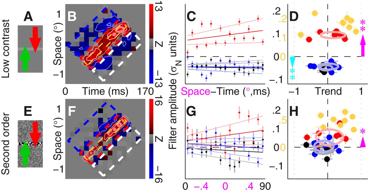
Trend effects are reduced by lowering contrast, and may not apply to second-order motion. B–D (low contrast; A, icon) and F–H (second order; E, icon) are plotted to the same conventions as Figure 2B–D. Yellow data in D and H (plotted to scale indicated by yellow numerals) refer to pooling regions indicated by dashed lines in B and F. See Materials and Methods for stimulus specifications.
The model in Figure 7B is not plausible at longer timescales, because the positive feedback loop would ultimately push gain outside the physiological range. Clearly, a stabilizing inhibitory feedback must operate beyond 100 ms. Our goal in this study was to characterize motion detectors on the timescale of their known temporal integration window of ∼100 ms (Burr, 1981); sensible resolution across this scale is in the order of 10 ms, as adopted here. With these parameters in mind, the associated dimensionality for the noise probe already stretched as far as could be feasibly characterized with the available data mass from our laboratory (we collected >400,000 trials for this study), making it impractical to study detector dynamics beyond 100 ms. We also wished to minimize any role for eye movements, a goal largely incompatible with longer-lasting stimuli. In a previous study (Neri and Levi, 2008), we focused our efforts on the properties of the motion sensor beyond detection, allowing us to channel probe energy directly into the motion dimension (we did not characterize space–time but rather bypassed the early detection stage altogether); because adequate temporal resolution for that study was on the scale of ∼30 ms, we were able to characterize dynamics over a window of 300 ms. Although those measurements did not probe spatiotemporal structure and are therefore only indirectly relevant to the present results, they provided evidence in favor of a negative feedback loop with a time delay of ∼90 ms (Neri and Levi, 2008, their Fig. 1E). A mechanism of this kind could serve to stabilize the network circuit in Figure 7B at longer timescales. It is particularly relevant in this context that related measurements from single neurons in primary visual cortex have revealed the existence of two mechanisms shaping population activity spread in response to motion-like stimulus sequences: early excitation operating within 45 ms of stimulus onset, followed by late inhibition (Jancke et al., 1999). These electrophysiological results are highly consistent with our previous (Neri and Levi, 2008) and current psychophysical findings, as well as with related behavioral findings from independent laboratories (Tadin et al., 2006; Iyer et al., 2011).
Is the dynamic effect specific to Fourier motion?
All experiments detailed so far used stimuli involving spatiotemporal modulations of luminance. There is evidence that this class of stimuli, often termed “first-order” in the literature (Lu and Sperling, 2001), relies on distinct perceptual circuitry not shared by “second-order” stimuli (Vaina and Soloviev, 2004), prompting us to determine whether the effects we found for first-order stimuli would extend to second-order motion. As demonstrated in Figure 8F–H, our primary analysis did not detect significant trend effects for a second-order contrast-based variant of the motion stimulus (Fig. 8H, red data points scatter around vertical dashed line at p = 0.3), despite the presence of measurable structure (Fig. 8H, red data points tend to fall above horizontal dashed line at p < 0.04).
Qualitative inspection of the aggregate filter (Fig. 8F) suggests that the central ridge may be narrower for the second-order experiments, making the analysis with tighter pooling space–time window (Fig. 8F, yellow dashed region) particularly relevant to this dataset. The analysis with narrow pooling region revealed nearly significant trend effects at p = 0.054 (Fig. 8H, yellow symbols). However, a word of caution is necessary in relation to this alternative analysis. Clearly, by selecting arbitrary subregions of the perceptual filter one can demonstrate any effect and its opposite. The specific choice initially adopted in Figure 2 was motivated by a reasonable attempt to partition the filter into regions of comparable size; trend effects for first-order stimuli were then validated on multiple occasions using the same analysis applied to independent datasets. We can therefore be confident that those effects are genuine and not a consequence of arbitrary choices associated with data analysis. In the case of the second-order dataset, we do not have access to independent replications and/or relevant experimental variants; because trend effects became mildly visible only by tailoring the analysis to this specific dataset, and in light of the associated p value failing to reach the significance cutoff of 0.05, at this stage we must conclude that trend effects are not supported by second-order motion mechanisms.
Can related effects be observed using substantially different stimuli and tasks?
An important question raised by the novel effect reported in this study is to what extent it may affect motion perception in general, i.e., whether it may apply to a very different family of motion stimuli and tasks. Clearly we cannot address this question for all possible specifications, but we can take a first step in this direction by considering a commonly studied stimulus class with associated discrimination task. We designed a composite random-dot motion stimulus consisting of two brief temporally juxtaposed segments: an 80 ms “inducer” segment containing exclusively upward-moving dots, and a 40 ms “test” segment containing a varying percentage of upward-moving dots with the remaining “signal” dots moving either to the left or to the right of upwards (left is shown by example stimulus in Fig. 9A). Observers were asked to indicate whether the composite stimulus, lasting 120 ms in total, displayed a tendency to move leftward or rightward. Mixed within the same block, we then presented two different stimulus configurations: test segment followed by inducer segment (“early-test”; Fig. 9B), or inducer segment followed by test segment (“late-test”; Fig. 9C; see also Materials and Methods). Because of the brief timescale involved, this manipulation was not perceptually conspicuous and observers were not aware of it.

Directional discrimination of random-dot stimuli is consistent with main results. A, Observers were asked to judge the direction (left vs right) of dots moving within a circular aperture. All dots moved upwards during the inducer segment (light colors in B and C), while a percentage of “signal” dots moved either left or right during the test segment (solid colors). Segment order was either test-inducer (“early” configuration, B) or inducer-test (“late,” C). D plots percentage of correct responses (aggregate across observers) as a function of signal-dot percentage for both early (black) and late trials (red) at high contrast; smooth lines show Weibull fits. E plots log-ratios between early and late configurations for best-fit scale (x-axis) and shape (y-axis) parameters at high (solid) and low (open) contrast. Error bars in D and E plot ±1 SEM.
The dynamic effects detailed above predict that the two stimulus configurations should be associated with different discrimination performance. More specifically, in the “late” configuration, a coherent motion signal is delivered by the inducer before test appearance; within the context of the modeling framework in Figure 7B, this signal would vigorously activate the positive gain-control module (orange diagrams), which in turn may be expected to engage and sensitize the entire motion-detection circuitry tuned for upward motion. Because no such prior engagement is afforded by the “early” configuration, it may be expected that performance should be poorer for this condition. This is indeed what we observed across the whole range of signal-to-noise ratios (Fig. 9D). Two-parameter (scale/shape) Weibull fits to individual observer data returned significantly reduced scale (threshold) values for the “late” configuration [Fig. 9E, solid data points fall to the right of vertical dashed line at p < 0.05; positive early/late log-ratio values indicate lower scale values (better thresholds) for the “late” configuration]. The shape parameter was not significantly affected by the early/late manipulation (Fig. 9E, solid data points scatter around horizontal dashed line at p = 0.84). These results are consistent with existing psychophysical studies on sequential recruitment of motion detectors (McKee and Welch, 1985; Verghese et al., 1999).
As detailed earlier, lowering contrast substantially reduced trend effects (Fig. 8A–D). If the threshold change associated with the early/late manipulation described here is at least partially connected with the earlier measurements, we may expect a reduction of this effect at lower stimulus contrast. Our measurements with lower-contrast random-dot stimuli did show a smaller threshold change to the extent that it was no longer significant (Fig. 9E, open data points scatter around vertical dashed line at p = 0.09). However, the effect was not entirely eliminated by lowering contrast. It is worth noticing two relevant issues in this respect. First, it is unclear that a fivefold change in contrast (as was used in these experiments) delivers comparable perceptual manipulations of contrast/visibility for the two stimulus classes used in Figure 8A–D and Figure 9; a wider contrast range should be tested in future experiments. Second, the lack of dynamic effects for the low-contrast bar stimulus used earlier may be due to heterogeneous behavior across participants (rather than lack of an effect for each participant), as suggested by the possibly bimodal scatter of red/yellow data points in Figure 8D; larger participant samples will be necessary to characterize contrast dependence adequately. In conclusion, our experiments with random-dot stimuli have exposed a relatively large and easily measurable effect of the early/late manipulation (Fig. 9D). However, further experimentation will be necessary to pinpoint its properties under varying stimulus specifications.
Discussion
Why has it not been reported before?
Before discussing in any detail the effects described here, we address the question of why they have gone unreported by previous studies. The human motion detector has been under intense scrutiny for several decades (Clifford and Ibbotson, 2002); it may therefore appear surprising that a robust 2–3× gain change of its oriented spatiotemporal characteristic has gone undetected. We believe the answer to this question is methodological. In most previous psychophysical characterizations of the human motion detector, its spatiotemporal structure has been measured indirectly via the corresponding power spectrum in the frequency domain (Burr and Ross, 1986; Reisbeck and Gegenfurtner, 1999). Although spectral estimates enabled previous research to uncover the oriented nature of the spatiotemporal filter (Burr et al., 1986; Anderson and Burr, 1989), they were not in a position to gauge the type of dynamics exposed by the present study: the power spectrum of surface P(x,t) in Figure 7A is identical to the power spectrum of P(x,−t), i.e., an increasing trend is indistinguishable from a decreasing trend when viewed in the phase-stripped frequency domain. Our methodology probes the motion detector directly in space–time, allowing us to expose the novel structure detailed in this study.
The above considerations appear inapplicable to single-unit electrophysiological research: direct spatiotemporal characterization of motion-sensitive cells using space–time noise probes has dominated the field (Emerson et al., 1987; Pack et al., 2006; Livingstone and Conway, 2007). Although motion-induced alterations of receptive field structure that may be relevant to the present results have been described (further discussed below), no consistent trend of the kind detailed here has been reported in this extensive literature. We believe this apparent discrepancy results from the different stages probed by psychophysical and electrophysiological investigations: electrode measurements may sample signals from any stage within the circuit in Figure 7B, possibly at the level of the front-end spatiotemporal filters. Psychophysical measurements, on the other hand, can only access the read-out stage. As demonstrated in Figure 6 and in line with the conclusions reached by relevant single-unit studies (Fu et al., 2004; Sundberg et al., 2006), the effects reported here most likely reflect dynamic properties introduced by network circuitry and not necessarily modifications at the level of front-end filtering. As such, these effects may not be available from electrophysiological measurements of cell responses.
Self-reinforcing feedback model
The model proposed in Figure 7B incorporates a positive feedback loop for gain control. Earlier psychophysical work has ascribed related phenomena to attentional capture (Neri and Heeger, 2002; Megna et al., 2012). However, this interpretation is unlikely to account for the results reported here. Amplitude of the central ridge increases steadily from stimulus onset, whereas exogenous attentional capture operates from ∼50–100 ms onwards (Nakayama and Mackeben, 1989; Ziebell and Nothdurft, 1999). Furthermore, the effect reported here is eliminated by surround stimulation (Fig. 4); there is no clear evidence that surround stimulation affects exogenous attention. Finally, attentional capture may be expected to produce more pronounced effects in the periphery compared with the fovea, yet we did not measure substantial differences between the two (Fig. 2). In conclusion, attentional interpretations of the effects reported here appear unsatisfactory.
A more likely explanation is that these effects reflect activity profiles associated with the progressive engagement of cortical circuitry. Recent results from connectivity studies indicate that later stages in the cortical processing hierarchy are substantially shaped not only by direct feedforward input, but also by the overall activation state of the extended circuit within which they are embedded (Yu and Ferster, 2013). Previous investigators have noted that this issue may be particularly relevant for reverse correlation studies where stimuli are expected to engage a larger fraction of the underlying circuitry, and that certain dynamic properties may be observed only or primarily under these conditions (Ringach and Shapley, 2004). The circuit in Figure 7B may therefore reflect a process whereby the human motion detector initially responds to stimulus onset, but subsequently engages only with stimuli that drive the motion-selective units effectively and contribute substantially to the additive pool that boosts gain.
Conceptually similar models have been proposed by previous investigators to explain related phenomena in retina (Berry et al., 1999), thalamus (Sillito et al., 1994), primary visual cortex (Jancke et al., 1999; Fu et al., 2004), extrastriate cortex (Mikami, 1992; Sundberg et al., 2006), and behavior (McKee and Welch, 1985; Verghese et al., 1999); although implementation details differ, these computational schemes share the underlying notion of what has been termed “asymmetric spread” (Kanai et al., 2004), “priming” (Sheth et al., 2000), “feedforward wave” (Baldo and Caticha, 2005), or “sequential recruitment” (McKee and Welch, 1985). There is overall consensus that this progressive activation of the motion-sensitive circuit, which may be interpreted as a rudimentary extrapolation mechanism (Baldo and Caticha, 2005) or locking/focusing device (Sillito et al., 1994), may be connected to a class of anticipatory perceptual phenomena. We discuss this potential connection below.
Potential significance for suprathreshold perception
In the flash-lag effect (FLE), the perceived spatial location of a moving bar is consistently mislocalized toward the direction of motion with respect to a static flashed bar (Hazelhoff and Wiersma, 1924; MacKay, 1961). It has been argued that this and related phenomenological effects (Fröhlich, 1930) may result from biased read-out of the motion detector (Krekelberg and Lappe, 2001; Eagleman and Sejnowski, 2007). To account for the observed direction of the phenomenological effects, such bias would need to allocate more perceptual weight to later epochs of the detector output (Nijhawan, 2002). The resulting trend would be broadly consistent with the dynamic structure reported in this study, offering a potential link with the phenomenological literature.
The above link is tentative and, at best, only applicable within limited contexts. FLEs occur for a wide range of stimuli, including second-order motion (Bressler and Whitney, 2006), cross-modal signals (Alais and Burr, 2003), and perceptual constructs unrelated to motion (Sheth et al., 2000; Bachmann and Põder, 2001), while the dynamic properties reported here may not extend much beyond first-order motion (Fig. 8E–H). Even when restricted to first-order signals, further consideration of relevant literature prompts caution: it is, for example, known that uncertainty can play a significant role in FLEs (Kanai et al., 2004), possibly accounting for their more pronounced nature in the periphery (Baldo et al., 2002; Fu et al., 2004). The dynamic structure reported here showed virtually no dependence on eccentricity (Fig. 2) and was unaffected by a relevant manipulation of spatial uncertainty: for the foveal condition with unoriented probes (Fig. 2I–K), we vertically shifted the stimulus by a random amount on every trial (within a ±45 arcmin range); trend effects were nonetheless measurable (Fig. 2K, yellow symbols).
Perceptual illusions and other important motion phenomena are typically demonstrated for stimuli not corrupted by noise (i.e., high stimulus signal-to-noise ratio). The mapping methodology used here requires near-threshold performance (Murray, 2011), making it difficult to extrapolate to conditions where perceived stimulus signal-to-noise ratio is high. We can gain some insight into this issue by considering that, were the measured effects on trend dependent on stimulus discriminability, we may expect a negative correlation between trend and discrimination performance (trend effects should be smaller for conditions/observers associated with higher stimulus discriminability). For the relevant experimental conditions (all except surround inhibition and low contrast), the d′ range spanned by our sample (58 estimates) was ∼0.5–1.4. Across this range there was no significant correlation with trend (p = 0.27), suggesting that trend effects may still be present at higher levels of stimulus discriminability. In line with this observation, our measurements of potentially relevant threshold effects with random-dot stimuli extended over a wide signal-to-noise ratio range (Fig. 9D).
The above conclusion, however, cannot be safely extrapolated to noiseless/uncorrupted stimuli associated with unhindered discriminability. It therefore remains to be determined to what extent, if at all, the characteristics we measured may relate to anticipatory motion illusions and more generally to suprathreshold conditions. Notwithstanding the speculative nature of their potential link to phenomenology, those characteristics retain a significance of their own, both in connection with the development of small-scale models for human motion detection (Clifford and Ibbotson, 2002), and in relation to their implications for directing further electrophysiological investigations into the underlying neural circuitry (Borst and Euler, 2011). Our results have exposed an unexpected property of human motion detectors. This property is robust and can be measured with high replicability (Figs. 2, 5, 7A), indicating that it may reflect structural characteristics of the underlying circuitry of fundamental importance to their operation under laboratory conditions. Further research will be necessary to elucidate its role and significance during natural vision.
Footnotes
This work was supported by the Royal Society of London, the Medical Research Council, and the CNRS (UMR8248).
The author declares no competing financial interests.
- Correspondence should be addressed to Peter Neri, Institute of Medical Sciences, University of Aberdeen, Foresterhill, Aberdeen AB25 2ZD, UK. neri.peter{at}gmail.com


