

Abstract
The mechanisms of reward maximization have been extensively studied at both the computational and neural levels. By contrast, little is known about how the brain learns to choose the options that minimize action cost. In principle, the brain could have evolved a general mechanism that applies the same learning rule to the different dimensions of choice options. To test this hypothesis, we scanned healthy human volunteers while they performed a probabilistic instrumental learning task that varied in both the physical effort and the monetary outcome associated with choice options. Behavioral data showed that the same computational rule, using prediction errors to update expectations, could account for both reward maximization and effort minimization. However, these learning-related variables were encoded in partially dissociable brain areas. In line with previous findings, the ventromedial prefrontal cortex was found to positively represent expected and actual rewards, regardless of effort. A separate network, encompassing the anterior insula, the dorsal anterior cingulate, and the posterior parietal cortex, correlated positively with expected and actual efforts. These findings suggest that the same computational rule is applied by distinct brain systems, depending on the choice dimension—cost or benefit—that has to be learned.
Introduction
Learning how to maximize rewards is one of the crucial abilities for the survival of species. Reinforcement learning (RL) models provide a reasonable computational account for reward maximization (i.e., the adaptation of behavioral choices across trials, based on past outcomes; Sutton and Barto, 1998; Dayan and Balleine, 2002). In basic RL models, learning is implemented by a delta rule (Rescorla and Wagner, 1972) that adjusts the expected value of the chosen option proportionally to prediction error (actual minus expected reward).
Neural signals of expected reward values and prediction errors were repeatedly found in the ventral corticostriatal circuit (O'Doherty et al., 2001; Pagnoni et al., 2002; Galvan et al., 2005; Hare et al., 2008; Rutledge et al., 2010), primarily in the ventromedial prefrontal cortex (vmPFC) and ventral striatum. The same delta rule can be applied to learning aversive values that drive avoidance behavior. Several studies have found evidence for a punishment system that signals aversive expected values and prediction errors, and which includes the anterior insula (AI) and dorsal anterior cingulate cortex (dACC; Büchel et al., 1998; Nitschke et al., 2006; Seymour et al., 2007; Samanez-Larkin et al., 2008; Palminteri et al., 2012).
While the neural signals involved in learning appetitive and aversive state values have been extensively studied, little is known about how the brain learns about costs such as the effort required to obtain a reward or the delay in reward delivery. These costs must be integrated to calculate the net value of each alternative and make a sound decision (Bautista et al., 2001; Walton et al., 2006; Berns et al., 2007; Kalenscher and Pennartz, 2008). In nonlearning contexts, previous evidence has shown that reward regions such as vmPFC integrate the negative value of delay, but the encoding of the effort cost has been more consistently observed in “aversive regions,” such as AI and dACC (Rudebeck et al., 2006; Kable and Glimcher, 2007; Prévost et al., 2010; Kurniawan et al., 2013; Meyniel et al., 2013).
These observations suggest that the effort cost might be processed by the brain in a particular way, perhaps because it is attached to actions and not to states. The question therefore arises of whether effort cost is learned through the same mechanisms as state values. Here, we monitored brain activity using fMRI while healthy participants performed an instrumental learning task in which choice options were probabilistically associated with various levels of effort and reward. Options were always left versus right button press, and contingencies were cued by an abstract symbol. All options were associated with a physical effort (high or low) leading to a monetary reward (big or small). Depending on the cue, left and right options differed either in the probability of high effort or in the probability of big reward. This design allowed us to compare the mechanisms driving reward maximization and effort minimization, at both the computational and neural levels.
Materials and Methods
Subjects.
The study was approved by the Pitié-Salpêtrière Hospital ethics committee. Participants were screened out for poor vision, left-handedness, age <18 and >39 years, history of psychiatric and neurological disorders, use of psychoactive drugs or medications, and contradictions to MRI scanning (metallic implants, claustrophobia, pregnancy). Twenty subjects (11 females; mean age, 24.0 ± 2.8 years) gave their written informed consent for participation in the study. To maintain their interest in the task, subjects were told that they would receive an amount of money corresponding to their performance. In fact, to avoid discrimination, payoff was rounded up to a fixed amount of 100€ for all participants, who were informed about it at the debriefing.
Behavioral data.
Subjects lay in the scanner holding in each hand a power grip made of two molded plastic cylinders compressing an air tube, which was connected to a transducer that converted air pressure into voltage. Isometric compression resulted in a differential voltage signal that was linearly proportional to the exerted force. The signal was transferred to a computer via a signal conditioner (CED 1401, Cambridge Electronic Design) and was read by a script using a library of Matlab functions named Cogent 2000 (Wellcome Trust for Neuroimaging, London, UK). Real-time feedback on the force produced was provided to subjects in the form of a mercury level moving up and down within a thermometer drawn on the computer screen. To measure maximal force, subjects were asked to squeeze the grip as hard as they could during a 15 s period. Maximal force (fmax) was computed as the average over the data points above the median, separately for each hand. The forces produced during the task were normalized by the maximal force of the squeezing hand, such that the top of the thermometer was scaled to fmax on both sides.
Before scanning, subjects received instructions about the task and completed a practice session. It was a probabilistic instrumental learning task with binary choices (left or right) and the following four possible outcomes: two reward levels (20 or 10¢) times two effort levels (80% and 20% of fmax). Reward and effort magnitudes were calibrated in pilot studies such that the average performance for the two dimensions was matched across subjects.
Every choice option was paired with both a monetary reward and a physical effort. Subjects were encouraged to accumulate as much money as possible and to avoid making unnecessary effort. Every trial started with a fixation cross followed by an abstract symbol (a letter from the Agathodaimon font) displayed at the center of the screen (Fig. 1A). When interrogation dots appeared on the screen, subjects had to make a choice between left and right options by slightly squeezing either the left or the right power grip. Once a choice was made, subjects were informed about the outcome (i.e., the reward and effort levels, materialized respectively as a coin image and a visual target; horizontal bar on the thermometer). Next a command, “GO!,” appeared on screen, and the bulb of the thermometer turned blue, triggering effort exertion. Subjects were required to squeeze the grip until the mercury level reached the target. At this moment, the current reward was displayed with Arabic digits and added to the cumulative total payoff. The two behavioral responses (choice and force) were self-paced. Thus, participants needed to produce the required force to proceed further, which they managed to achieve on every trial. Random time intervals (jitters), drawn from a uniform distribution between 1000 and 3000 ms, were added to cue and outcome presentations to ensure better sampling of the hemodynamic response.
Subjects were given no explicit information about the stationary probabilistic contingencies that were associated with left and right options, which they had to learn by trial and error. The contingencies were varied across contextual cues, such that reward and effort learning were separable, as follows: for each cue the left and right, options differed either in the associated reward or in the associated effort (Fig. 1B). For RL cues, the two options had distinct probabilities of delivering 20 versus 10¢ (75% vs 25% and 25% vs 75%), while probabilities of having to produce 80% versus 20% of fmax were identical (either 100% vs 100% or 0% vs 0%). Symmetrical contingencies were used for effort learning cues, with distinct probabilities of high effort (75% vs 25% and 25% vs 75%) and unique probability of big reward (100% vs 100% or 0% vs 0%). The four contextual cues were associated with the following contingency sets: reward learning with high effort; reward learning with low effort; effort learning with big reward; and effort learning with small reward. The best option was on the right for one reward learning and one effort learning cues, and on the left for the two other cues. The associations between response side and contingency set were counterbalanced across sessions and subjects. Each of the three sessions contained 24 presentations of each cue, randomly distributed over the 96 trials, and lasted about 15 min. The four symbols used to cue the contingency sets changed for each new session and had to be learned from scratch.
A model-free analysis was performed on correct choices using logistic regression against the following factors: learning dimension (reward vs effort); correct side (left and right); trial number; and the three interaction terms. Correct choice was defined as the option with the highest expected reward or the lowest expected effort. Individual parameter estimates (betas) for each regressor of interest were brought to a group-level analysis and tested against zero, using two-tailed one-sample t tests. To ensure that the manipulation of effort level was successful, we compared the force produced after low-effort outcome (Flow) and high-effort outcome (Fhigh). The difference was significant [Flow = 0.037 ± 0.005 arbitrary units (a.u.); Fhigh = 0.212 ± 0.0 a.u.; t(1,19) = 11.59; p < 0.001]. We also observed a small but significant difference in the effort duration (low-effort duration = 470 ± 22 ms; high-effort duration = 749 ± 66 ms; t(1,19) = −5.46; p < 0.001). Yet this difference was negligible compared with the total delay between cue and reward payoff (6402 ± 92 ms).
Computational models.
The model space was designed to investigate whether subjects used similar computations when learning to maximize their payoff and minimize their effort. We tested three types of learning models: ideal observer (IO); Q-learning (QL); and win-stay-lose-switch (WSLS). All models kept track of the reward and effort expectations attached to every choice option. In a learning session, there were eight options (four contextual cues × two response sides). The IO model simply counts the events and updates their frequencies after each choice. The expectations attached to each choice option are therefore the exact frequencies of big reward and high effort. The QL model updates expectations attached to the chosen option according to the following delta rule: QR(t + 1) = QR(t) + αR × PER(t) and QE(t + 1) = QE(t) + αE × PEE(t), where QR(t) and QE(t) are the expected reward and effort at trial t, αR and αE are the reward and effort learning rates, and PER(t)and PEE(t) are the reward and effort prediction errors at trial t. PER and PEE were calculated as PER(t) = R(t) − QR(t) and PEE(t) = E(t) − QE(t), where R(t), and E(t) are the reward and effort outcomes obtained at trial t. R and E were coded as 1 for big reward and high effort (20¢ and 80% of fmax), and as 0 for small reward and low effort (10¢ and 20% fmax). All Q values were initiated at 0.5, which is the true mean over all choice options. The WSLS model generates expectations based on the last outcome only. This model corresponds to an extreme version of the QL model (with a learning rate equal to 1). The combination of these models gives a total of nine possibilities, as any of the three models could be used for reward and effort learning. In the case where QL was applied to both reward and effort, we also tested the possibility of a shared learning rate (αE = αR), making a total of 10 combinations.
The three models differ in their learning rule, and, therefore, in the trial-by-trial estimates of reward and effort expectations attached to left and right options. The next step is to combine reward and effort expectations to calculate a net value for each option. We tested the following two discounting rules: a linear function for simplicity, and a hyperbolic function by analogy with delay-discounting models (Kable and Glimcher, 2007; Prévost et al., 2010; Peters and Büchel, 2011). Net values were calculated as Q(t) = QR(t) − γ × QE(t) or Q(t) = QR(t)/(1 + k × QE(t)), where γ and k are the linear and hyperbolic discount factors, respectively. We set the discount factors to be positive, given the vast literature showing that effort is aversive, and the model-free analyses of the present data showing that subjects tend to avoid high efforts. Finally, the net values of the two choice options had to be compared to generate a decision. We used a softmax rule, which estimates the probability of each choice as a sigmoid function of the difference between the net values of left and right options, as follows: PL(t) = 1/(1 + exp((QR(t) − QL(t))/β)), where β is a temperature parameter that captures choice stochasticity. Overall, the model space included 20 possibilities (10 combinations for the learning rule × two discounting rules) that could be partitioned into families that differed in the following three dimensions: (1) learning rule (IO, QL, or WSLS); (2) discounting rule (linear or hyperbolic); and (3) learning rate (same or different). All models were first inverted using a variational Bayes approach under the Laplace approximation (Daunizeau et al., 2014). This iterative algorithm provides approximations for both the model evidence and the posterior density of free parameters. As model evidence is difficult to track analytically, it is approximated using variational free energy (Friston and Stephan, 2009). This measure has been shown to provide a better proxy for model evidence compared with other approximations such as Bayesian Information Criterion or Akaike Information Criterion (Penny, 2012). In intuitive terms, the model evidence is the probability of observing the data given the model. This probability corresponds to the marginal likelihood, which is the integral over the parameter space of the model likelihood weighted by the priors on free parameters. This probability increases with the likelihood (which measures the accuracy of the fit) and is penalized by the integration over the parameter space (which measures the complexity of the model). The model evidence thus represents a tradeoff between accuracy and complexity, and can guide model selection.
The log evidences estimated for each model and each subject were submitted to a group-level random-effect analysis (Penny et al., 2010). This analysis provides estimates of expected frequency and exceedance probability (xp) for each model and family in the search space, given the data gathered from all subjects (Stephan et al., 2009; Rigoux et al., 2014). Expected frequency quantifies the posterior probability (i.e., the probability that the model generated the data for any randomly selected subject). This quantity must be compared with chance level (one over the number of models or families in the search space). Exceedance probability quantifies the belief that the model is more likely than the other models of the set, or, in other words, the confidence in the model having the highest expected frequency. The same best model was identified either by comparing all single models or by taking the intersection of the winning families.
To ensure that the best model provided a similar fit of reward and effort learning curves, we computed intersubject and intertrial correlations between observed and predicted choices. Individual free parameters (mean ± SEM: αR = 0.50 ± 0.04; αE = 0.39 ± 0.05; γ = 0.95 ± 0.24; and β = 2.12 ± 0.30) were used to generate trial-by-trial estimates of reward and effort expectations and prediction errors, which were included as parametric modulators in the general linear models (GLMs) designed for the analysis of fMRI data.
fMRI data.
T2*-weighted echoplanar images (EPIs) were acquired with BOLD contrast on a 3.0 T magnetic resonance scanner (Trio, Siemens). A tilted-plane acquisition sequence was used to optimize sensitivity to BOLD signal in the orbitofrontal cortex (Deichmann et al., 2003; Weiskopf et al., 2006). To cover the whole brain with sufficient temporal resolution (TR, 2 s), we used the following parameters: 30 slices; 2 mm thickness; and 2 mm interslice gap. Structural T1-weighted images were coregistered to the mean EPI, segmented and normalized to the standard T1 template, and then averaged across subjects for anatomical localization of group-level functional activation. EPIs were analyzed in an event-related manner, using general linear model analysis, and were implemented in the statistical parametric mapping (SPM8) environment (Wellcome Trust Center for NeuroImaging, London, UK). The first five volumes of each session were discarded, to allow for T1 equilibration effects. Preprocessing consisted of spatial realignment, normalization using the same transformation as anatomical images, and spatial smoothing using a Gaussian kernel with a full-width at a half-maximum of 8 mm.
Individual time series of preprocessed functional volumes were regressed against the following main GLM (i.e., GLM1). Five categorical regressors were included as indicator functions modeling the onsets of (1) cue presentation, (2) motor response, (3) outcome presentation, (4) squeezing period, and (5) payoff screen. In addition, the following five parametric regressors were added: expected reward and effort from the chosen option (QR and QE) at cue onset, the chosen option (−1 for left and 1 for right) at response time, and PER and PEE at outcome onset. Note that predictions and prediction errors were modeled for all cues and outcomes (i.e., even when they could not be used to improve choices; because the two responses were equivalent). All regressors of interest were convolved with the canonical hemodynamic response function. To correct for motion artifact, subject-specific realignment parameters were modeled as covariates of no interest.
Regression coefficients were estimated at the single-subject level using the restricted maximum-likelihood estimation. Linear contrasts of regression coefficients were then entered in a random-effect group-level analysis (one-sample paired t test). All main activations reported in the text survived a cluster-extent FWE-corrected threshold of p < 0.05. Primary contrasts of interest were parametric modulations by expected reward and effort, and the difference between them, as they were assumed to reflect the learning process. Formal conjunction analyses were performed to test for simultaneous encoding of both expected reward and effort. Regression coefficients (β estimates) were extracted from significant functional clusters in whole-brain group-level contrasts. To test for the encoding of prediction errors, one-sample t tests were performed on β estimates extracted from the clusters of interest, which were identified using an independent contrast.
We ran several additional GLMs to confirm the results and to assess supplementary hypotheses. In GLM2, we replaced the two regressors modeling expected reward and effort with a single regressor modeling the net chosen value to confirm the activation maps showing brain regions that encode expected reward and effort with an opposite sign. In GLM3, we replaced the chosen value regressors with regressors modeling the difference between chosen and unchosen values to assess whether the clusters of interest encoded a differential value signal. In GLM4, we split trials based on the left and right choice, and replaced the regressors modeling chosen values by regressors modeling expected reward and effort for left and right options separately to test for lateralization of value coding. In any case, we kept other regressors identical to the main model (GLM1).
Results
Behavior
A model-free analysis of correct choices using logistic regression showed a significant main effect of trial number (t(1,19) = 3.75, p = 0.007) with no effect of learning dimension (reward vs effort) or correct side (left vs right) and no interaction. This indicates that learning performance was similar for reward and effort (Fig. 1C), and independent from the hand to which the correct response was assigned. We checked that learning was not dependent on the other dimension by comparing performance between contingency sets corresponding to the different cues. Specifically, there was no significant difference in reward learning between high- and low-effort conditions (cue A vs B: t(1,19) = 0.94, p = 0.36), and no significant difference in effort learning between big and small reward conditions (C vs D: t(1,19) = 0.49, p = 0.63).
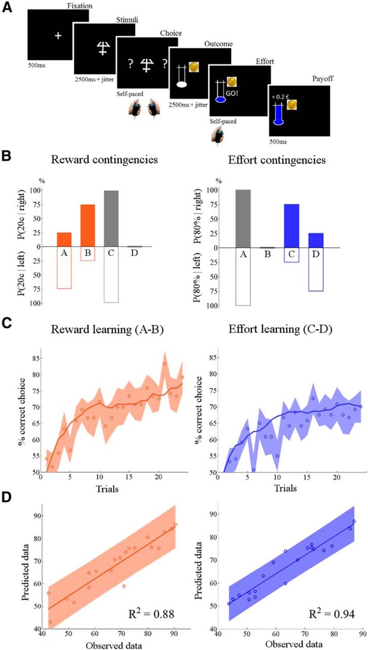
Behavioral task and results. A, Trial structure. Each trial started with a fixation cross followed by one of four abstract visual cues. The subject then had to make a choice by slightly squeezing the left or right hand grip. Each choice was associated with two outcomes: a monetary reward and a physical effort. Rewards were represented by a coin (10 or 20¢) that the subject received after exerting the required amount of effort, indicated by the height of the horizontal bar in the thermometer. The low and high bars corresponded respectively to 20% and 80% of a subject's maximal force. Effort could only start once the command GO! appeared on the screen. The subject had to squeeze the handgrip until the mercury reached the horizontal bar. In the illustrated example, the subject made a left-hand choice and produced an 80% force to win 20¢. The last screen informed the subject about the gain added to cumulative payoff. B, Probabilistic contingencies. There were four different contingency sets cued by four different symbols in the task. With cues A and B, reward probabilities (orange bars) differed between left and right (75%/25% and 25%/75%, respectively, chance of big reward), while effort probabilities (blue bars) were identical (100%/100% and 0%/0%, respectively, chance of big effort). The opposite was true for cues C and D: left and right options differed in effort probability (75%/25% and 25%/75%, respectively) but not in reward probability (100%/100% and 0%/0%, respectively). The illustration only applies to one task session. Contingencies were fully counterbalanced across the four sessions. C, Learning curves. Circles represent, trial by trial, the percentage of correct responses averaged across hands, sessions, and subjects for reward learning (left, cues A and B) and effort learning (right, cues C and D). Shaded intervals are intersubject SEM. Lines show the learning curves generated by the best computational model (QL with linear discount and different learning rates for reward and effort) identified by Bayesian model selection. D, Model fit. Scatter plots show intersubject correlations between estimated and observed responses for reward learning (left) and effort learning (right). Each dot represents one subject. Shaded areas indicate 95% confidence intervals on linear regression estimates.
To refine the comparison between reward and effort learning, we estimated 20 models (Table 1) that differed in the learning rule used to update the estimates of reward and effort attached to the different cues, and in the discounting function used to scale the positive effect of reward and the negative effect of effort on choices. Bayesian model selection over the families of models with different learning rules identified the QL model as giving the best account for both reward and effort learning compared with the IO or WSLS model (with xp = 0.97). Within the family of models that used QL for both reward and effort, those with distinct learning rates were selected as far more plausible (xp = 0.99). Direct comparison using a paired t test confirmed that posterior learning rates were higher for reward than for effort (mean ± SEM, 0.50 ± 0.04 vs 0.39 ± 05; t(1,19) = 2.91; p = 0.01). Comparison of the two families with different discounting functions revealed that linear discounting of reward by effort was preferable to hyperbolic discounting (xp = 0.99). When comparing all single models, the most plausible one was again the model using QL for both reward and effort, with distinct learning rates, and linear discounting (xp = 0.87). This model contains four free parameters (reward and effort learning rates, discount factor, and choice temperature).
Bayesian model comparison
To summarize, model comparison suggests that the most plausible computational mechanism underlying learning performance is the following. At the time of the outcome, both the reward and effort associated with the chosen option are updated in proportion to the reward and effort prediction errors, according to a Rescorla–Wagner rule. Then, at the time of cue onset, the net values of left and right options are estimated through linear discounting of the expected reward by the expected effort, and choice is made by selecting the higher net value with a probability given by the softmax function. The fact that the same mechanism was used for reward and effort learning suggests that the same brain system might learn the two dimensions. However, the fact that distinct learning rates were used rather hints that separate brain systems might be involved, even if they implemented the same computations.
To disentangle these hypotheses using fMRI data, it was important to check first that the winning computational model provided an equally good fit of reward and effort learning. Figure 1C illustrates the fit of choice data averaged across subjects, using the posterior parameter estimates obtained from group-level fixed-effect inversion (meaning that the same parameters were used for all subjects, as in the analysis of fMRI data). The intertrial correlations between predicted and observed choices were similar for reward and effort learning (R2 = 0.87 and 0.82, respectively; both p < 0.01). Figure 1D illustrates the correlations across subjects, between observed and predicted choices using individual parameters. Again correlations were similar for reward and effort learning (R2 = 0.88 and 0.94, respectively; both p < 0.01).
Neuroimaging
We first looked for brain regions tracking the reward and effort estimates through learning sessions. BOLD signal time series were regressed against the reward and effort expected from the chosen option, modeled at the time of cue onset (QR and QE in GLM1; see Materials and Methods). Table 2 provides a list of all significant activations, both at a liberal threshold of p < 0.001 uncorrected and at a stringent threshold of p < 0.05, FWE corrected at the cluster level. Focusing on the corrected threshold, we found that expected reward was positively encoded in the vmPFC (Fig. 2A). Activity in this region was not influenced by expected effort. More generally, we found no brain area showing any effect of expected effort in addition to positive correlation with expected reward, even at a very liberal threshold (p < 0.01, uncorrected). However, there were regions showing both negative correlation with expected reward and positive correlation with expected effort (Fig. 2B). These regions encompass the dACC with extension to the supplementary motor area, the right AI, the right posterior parietal cortex (PPC), and the dorsal occipital cortex. Similar clusters were found in the negative correlation with the net value modeled in a single regressor (Q = QR − γ × QE in GLM2; see Materials and Methods). There was no region showing increased activation in response to decreasing expected efforts, even at a liberal threshold (p < 0.01, uncorrected).
Brain activations
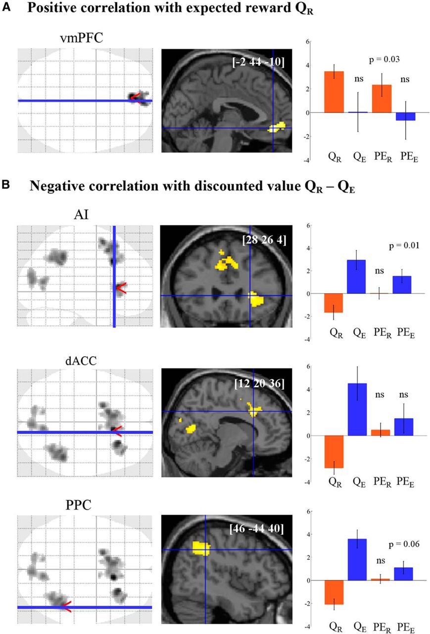
Neural underpinnings or effort and reward learning. A, B, Statistical parametric maps show brain regions where activity at cue onset significantly correlated with expected reward (A) and with the difference between expected effort and reward (B) in a random-effects group analysis (p < 0.05, FWE cluster corrected). Axial and sagittal slices were taken at global maxima of interest indicated by red pointers on glass brains, and were superimposed on structural scans. [x y z] coordinates of the maxima refer to the Montreal Neurological Institute space. Plots show regression estimates for reward (orange) and effort (blue) prediction and prediction errors in each ROI. No statistical test was performed on the β-estimates of predictions, as they served to identify the ROIs. p values were obtained using paired two-tailed t tests. Errors bars indicate intersubject SEM. ns, Nonsignificant.
Formal conjunction analyses were used to identify regions that simultaneously encoded reward and effort estimates (Nichols et al., 2005). The only conjunction that yielded significant activations was the negative correlation with expected reward coupled with the positive correlation with expected effort. In this conjunction, only the PPC survived the FWE-corrected clusterwise threshold. The right AI and the dACC clusters were observed at p < 0.001 (uncorrected). The other conjunctions confirmed that no brain region encoded the two dimensions with the same sign. There was no region showing positive encoding of net value (positive correlation with expected reward coupled with negative correlation with expected effort). Thus, our results bring evidence for partially distinguishable brain networks, with one region encoding expected rewards (vmPFC) and a set of other regions encoding negative net values (dACC, AI, PPC). This dissociation was also obtained when using the same learning rates for reward and effort. It was therefore driven by the difference in the content (reward vs effort) and not in the timing of learning.
We tested several variants of the regressors modeling expected values. First, we examined whether the brain encodes a differential signal (chosen − unchosen value in GLM3; see Materials and Methods) instead of just reflecting expectations. We obtained almost identical results to those of GLM1, with the vmPFC for expected reward and the same network (dACC, AI, PPC) for negative net value. However, these effects were driven by the chosen value, as the correlation with the unchosen value alone was not significant. Second, we tested whether the value signal could be spatially framed (with regressors for left and right values in GLM4; see Materials and Methods). We did not observe any lateralization effect, neither for expected reward nor for expected effort. Together, these results suggest that the clusters identified above encoded expected values (reward and effort level associated with the chosen option) and not decision or action values, which should be attached to the option side or the motor effector (left vs right).
To assess whether these regions were also implicated in updating reward and effort estimates, we tested the correlation with reward and effort prediction error signals at the moment of outcome display. Regression coefficients (β values) were extracted from all the clusters that survived the corrected threshold in the group-level analysis (Fig. 2). Note that the contrasts used to define the clusters of interest (correlations with expected reward and negative net value) were independent from the correlation with the prediction errors tested here.
Activity in the vmPFC was found to positively signal reward prediction errors (t(1,19) = 2.36, p = 0.03), but not effort predictions errors (t(1,19) = 0.40, p = 0.69). Conversely, activity in the right AI showed positive correlation with effort prediction errors (t(1,19) = 2.52, p = 0.01), but not with reward prediction errors (all p > 0.5). The same trend was observed in the PPC but did not reach significance (t(1,19) = 1.96, p = 0.06). There was no significant encoding of effort prediction errors within the dACC (t(1,19) = 1.13, p = 0.27).
Other regions were found to reflect prediction errors at the whole-brain level (Table 2), notably the ventral striatum, posterior cingulate cortex, occipital cortex, thalamus, and cerebellum for reward prediction errors, and the superior temporal gyrus, occipital cortex, and thalamus for effort prediction errors. In another GLM, we split the prediction error term with outcome (reward and effort) and prediction (expected reward and effort) in separate regressors. Only the outcome part was significantly encoded in our ROI, with reward in the vmPFC (t(1,19) = 4.13, p = 0.0006), and effort in the AI (t(1,19) = 2.72, p = 0.014), dACC (t(1,19) = 2.13, p = 0.04), and PPC (t(1,19) = 4.62, p = 0.0002). Thus, while our data suggest that reward and effort regions are sensitive to reward and effort outcomes (respectively), they remain inconclusive about whether these regions truly encode signed prediction errors.
Discussion
We explored the computational principles and neural mechanisms underlying simultaneous learning of reward and effort dimensions. In principle, the brain could have evolved a general learning mechanism applying the same process to update any choice dimension. Consistently, choice behavior suggested that the same computational process could equally account for reward maximization and effort minimization. However, neuroimaging data revealed that the brain systems underlying reward and effort learning might be partially dissociable.
The capacity of delta rules (also called Rescorla–Wagner rules) to account for learning behavior has been shown previously in a variety of domains, not only reward approach and punishment avoidance, but also the monitoring of perceptual features or social representations (Behrens et al., 2008; Preuschoff et al., 2008; Law and Gold, 2009; den Ouden et al., 2009; Zhu et al., 2012). These delta rules may represent a domain-general form of learning applicable to any choice dimension with stable or slowly drifting values (Nassar et al., 2010; Trimmer et al., 2012; Wilson et al., 2013). The present study extends this notion by showing that the same delta rule provides an equally good fit of reward and effort learning. We compared the delta rule to the ideal observation, which means counting the events and computing an exact frequency. The ideal observer thereby implements an adaptive learning rate, as it puts less weight on the new observation relative to previous ones. At the other extreme of the spectrum, we have the win-stay-lose-switch strategy, which takes only the last observation into consideration. The delta rule was identified as the most plausible model in the Bayesian selection, even if it was penalized for having an extra free parameter (the learning rate).
Another conclusion of the model selection is that subjects discounted linearly reward with effort. This may seem at odds with the literature on cost discounting showing the advantages of hyperbolic or quasi-hyperbolic models over simpler functions (Loewenstein and Prelec, 1992; Green et al., 1994; Prévost et al., 2010; Minamimoto et al., 2012; Hartmann et al., 2013). A key difference between the present task and standard delay and effort discounting paradigms is that the attributes of choice options (reward and effort levels) were not explicitly cued, but instead had to be learned by trial and error. However, the winning model in the Bayesian comparison had distinct learning rates for reward and effort. Note that the discount factor already explained the different weights that reward and effort had on choice. This scaling parameter was necessary as there was no reason to think a priori that the reward levels should be directly comparable to effort levels. The fact that, in addition to the discount factor, a good fit needed distinct learning rates, suggests that participants were faster to maximize reward than to minimize effort. Of course we do not imply that the reward learning system is intrinsically faster than the effort learning system. Here, subjects might have put a priority on getting the high reward, with less emphasis on avoiding high effort. It is likely that priorities could be otherwise in different environments, where for instance fatigue would be more constraining.
We nevertheless acknowledge that the model space explored in our comparison was rather limited. In particular, we did not test more complex architectures that would track higher-order dynamics (Hampton et al., 2006; Behrens et al., 2007; Mathys et al., 2011; Doll et al., 2012). This is because higher-order dynamics would not give any advantage in our environment, which had a null volatility. Also, the complexity of task structure, with four sets of contingencies linking the four cues to the four outcomes, makes the construction of explicit representations quite challenging. At debriefing, none of the subjects but one could report the key task feature, namely that only one dimension (reward or effort) differed between the choice options. This suggests that participants have built and updated both reward and effort estimates in all conditions (i.e., for every cue). Thus, we believe we have set a situation where reward and effort are learned using the same simple computations, which enables asking the question of whether in this case the same brain systems are engaged.
The primary objective of the neuroimaging data analysis was to identify the regions that track the expected reward and effort given the chosen option. These expectations are the quantities that are updated after the outcome, and thereby are the main correlates of learning. We did not observe any activity that would be correlated to reward and effort with the same sign, which validates the assumption that these two quantities are processed in an opponent fashion. The representation of expected reward was localized principally in the vmPFC, a brain region that has been classically implicated in positive valuation of choice options (Rangel et al., 2008; Haber and Knutson, 2010; Peters and Büchel, 2010; Levy and Glimcher, 2012; Bartra et al., 2013). This finding is also consistent with the observation that damage to the vmPFC impairs reward learning in humans and monkeys (Camille et al., 2011; Noonan et al., 2012; Rudebeck et al., 2013). Effort was absent from the expectations reflected in the vmPFC, which is in keeping with previous findings in nonlearning contexts that the vmPFC discounts rewards with delay or pain, but not with effort (Kable and Glimcher, 2007; Peters and Büchel, 2009; Talmi et al., 2009; Plassmann et al., 2010; Prévost et al., 2010). This might be linked to the idea that the vmPFC encodes value in the stimulus space, and not in the action space (Wunderlich et al., 2010). Also consistent with this idea is the absence of lateralization in reward representations associated with left and right responses, which was observed in a previous study (Palminteri et al., 2009) where the two options were associated with left and right cues on the computer screen. Other studies have shown lateralization of action value representations in motor-related areas but not in orbitofrontal regions (Gershman et al., 2009; Madlon-Kay et al., 2013).
A separate set of brain regions was found to represent expected effort, as well as the following negative reward: the anterior insula; the dorsal anterior cingulate cortex; and the posterior parietal cortex. These regions have already been implicated in the representation of not only effort but also negative choice value during nonlearning tasks (Bush et al., 2002; Samanez-Larkin et al., 2008; Croxson et al., 2009; Prévost et al., 2010; Hare et al., 2011; Burke et al., 2013; Kurniawan et al., 2013). The dissociation of vmPFC from dACC is reminiscent of the rodent studies reporting that after a cingulate (but not orbitofrontal) lesion physical cost is no longer integrated into the decision value (Walton et al., 2003; Roesch et al., 2006; Rudebeck et al., 2006), although this analogy should be taken with caution due to anatomical differences between species. As the net value expressed in this network was attached to the chosen option, and not to the difference between option values, it is unlikely to participate in the decision process. It might rather represent an anticipation of the outcomes that later serve to compute prediction errors.
The neural dissociation made for expectations at cue onset was also observed in relation to outcomes. Whereas the reward region (vmPFC) reflected reward prediction errors, the negative value network (at least AI) reflected effort prediction errors. This fits with a predictive coding account of brain architecture, in which regions that estimate a given dimension of the environment reflect both predictions and prediction errors (Rao and Ballard, 1999; Friston, 2005; Spratling, 2010). While all our ROIs were undoubtedly sensitive to outcomes, we found no clear evidence that they encoded signed prediction errors. It remains possible that they implement other computations integrating the outcomes, for instance unsigned prediction errors, as was previously observed in dACC single units (Bryden et al., 2011; Hayden et al., 2011; Klavir et al., 2013). In more dynamic environments, these signals might be used at a meta-cognitive level to regulate learning rate or choice temperature (Pearce and Hall, 1980; Doya, 2002; Khamassi et al., 2013). Also, the fact that neural activity in ROIs such as vmPFC and AI correlated with prediction errors does not imply that these regions compute prediction errors. While the reward prediction errors in the positive valuation system have been linked to dopamine release (Schultz et al., 1997; Frank et al., 2004; Pessiglione et al., 2006), the origin of effort prediction error signals is less clear. Animal studies have suggested that dopaminergic activity does not integrate effort cost, a pattern that we observed here in vmPFC activity (Walton et al., 2005; Gan et al., 2010; Pasquereau and Turner, 2013). Further studies are needed to examine whether dopamine or other neuromodulators might have an impact on effort prediction errors in humans.
More generally, our findings support the existence of multiple brain learning systems that have evolved to track different attributes of choice options, through similar computational mechanisms. Dissection of independent and joint nodes within positive and negative value systems may contribute to a better understanding of neuropsychiatric symptoms such as apathy, which in principle could arise from either insensitivity to potential rewards or overestimation of required efforts.
Footnotes
The study was funded by a Starting Grant from the European Research Council (ERC-BioMotiv). This work was also supported by the “Investissements d'Avenir” program (Grant ANR-10-IAIHU-06). V.S. received a PhD fellowship from the Ecole de Neurosciences de Paris, and S.P. received support from the Neuropôle de Recherche Francilien. We thank Maël Lebreton for his help in data acquisition; and Lionel Rigoux and Florent Meyniel for their help in data analysis.
The authors declare no competing financial interests.
- Correspondence should be addressed to Mathias Pessiglione, Institut du Cerveau et de la Moelle Épinière, Hôpital de la Pitié-Salpêtrière, 47 Boulevard de l'Hôpital, 75013 Paris, France. mathias.pessiglione{at}gmail.com


