

Abstract
The spatial topography of visual attention is a distinguishing and critical feature of many theoretical models of visuospatial attention. Previous fMRI-based measurements of the topography of attention have typically been too crude to adequately test the predictions of different competing models. This study demonstrates a new technique to make detailed measurements of the topography of visuospatial attention from single-voxel, fMRI time courses. Briefly, this technique involves first estimating a voxel's population receptive field (pRF) and then “drifting” attention through the pRF such that the modulation of the voxel's fMRI time course reflects the spatial topography of attention. The topography of the attentional field (AF) is then estimated using a time-course modeling procedure. Notably, we are able to make these measurements in many visual areas including smaller, higher order areas, thus enabling a more comprehensive comparison of attentional mechanisms throughout the full hierarchy of human visual cortex. Using this technique, we show that the AF scales with eccentricity and varies across visual areas. We also show that voxels in multiple visual areas exhibit suppressive attentional effects that are well modeled by an AF having an enhancing Gaussian center with a suppressive surround. These findings provide extensive, quantitative neurophysiological data for use in modeling the psychological effects of visuospatial attention.
Introduction
It has long been known from behavioral tests that visual attention can alter information processing in a spatially specific manner within the visual field (James, 1890; von Helmholtz, 1909; Wundt, 1924/1896; Eriksen and St James, 1986; Posner et al., 1980). These observations and the presence of retinotopic maps in visual cortex (Inouye, 1909; Holmes, 1918; Wandell and Winawer, 2011) led to the suggestion that visuospatial attention acts by modulating neuronal responses at retinotopically appropriate regions within cortical visual areas. Single-cell studies performed in monkeys supported this by showing that neurons exhibited increased firing rates when attention was directed to a spatial location within their receptive fields (RFs) (Motter, 1993; Treue and Maunsell, 1999). Neuroimaging studies performed in humans have provided further support by demonstrating that enhancement of cortical activity moves in register with shifts of visual attention (Tootell et al., 1998; Brefczynski and DeYoe, 1999; Gandhi et al., 1999; Silver et al., 2005).
The notion that the spatial distribution of attentional effects has a definable topography is central to many theoretical models of visual attention including the spotlight (Posner et al., 1980), zoom lens (Eriksen and Yeh, 1985), gradient (Downing and Pinker, 1985), and normalization (Reynolds and Heeger, 2009) models of attention. The fact that the topography of attention is a critical component of such models, and often a distinguishing feature among them, underscores the necessity of accurately measuring the spatial topography of attentional effects not only behaviorally but also neurophysiologically in terms of the patterns of cortical modulation.
Attentional field mapping was developed to estimate the topography of visual attention from patterns of cortical modulation (Brefczynski-Lewis et al., 2009; Datta and DeYoe, 2009). This technique works well in larger visual areas with well defined retinotopic maps (e.g., V1). However, it relies on reconstructing a pattern of activation using multiple voxels and is thus limited by the coarse voxel sampling of cortical space and the presence of local susceptibility artifacts. Both issues are exaggerated in higher order visual areas due to their smaller size (Puckett et al., 2010). Since different cortical visual areas are functionally specialized (Zeki et al., 1991; Maunsell, 1992; DeYoe and Van Essen, 1995; Haxby et al., 2001) and since attention influences processing in most, if not all, visual areas (Treue, 2001; DeYoe and Brefczynski, 2005; Li et al., 2008; Lauritzen et al., 2010; Bressler et al., 2013), a comprehensive neurophysiological model of attention must encompass the full hierarchy of cortical visual areas and their individual attentional effects.
Here, we developed a technique to measure the topography of visual attention using single voxels. In 2008, Dumoulin and Wandell showed that if a stimulus was swept across the population receptive field (pRF) of a voxel, the resulting fMRI time course reflected the combined spatial characteristics of the pRF and the stimulus. Through the use of modeling, it was possible to estimate the spatial profile of the pRF from the voxel's fMRI response (Dumoulin and Wandell, 2008). We report an analogous method to measure the topography of the attentional field (AF) from single-voxel fMRI responses.
Materials and Methods
Subjects.
Four male, right-handed subjects (ages 25–61) with normal or corrected-to-normal vision and no history of neurological or psychiatric diseases participated in the experiments. Experiments were conducted with the informed written consent of each observer and performed in accordance with procedures approved by the Institutional Review Board of the Medical College of Wisconsin.
Visual stimuli.
Visual stimulation was presented using a custom back-projection screen mounted on the MR head coil. A ViSaGe MKII visual stimulus generator by Cambridge Research was used in conjunction with MATLAB to drive a BrainLogics BLMRDP-A05 MR digital projector. The outer margin of the circular visual display extended to 20° eccentricity.
The multisegment array used for both attention and control conditions (Fig. 1A,B) consisted of a fixation marker superimposed on a center segment surrounded by five rings of segments centered at eccentricities 1, 2, 4, 8, and 16°. Each ring was scaled in size with eccentricity and divided into 12 segments of equal width. Only a fine gap separated segments producing a nearly contiguous array. Each segment contained a 7.5 Hz counterphase flickering square wave grating pattern, which changed orientation and/or color randomly every 2 s. The grating pattern scaled with eccentricity and consisted of horizontal or vertical bars that were either red and dark gray or green and dark gray. The array was displayed on a uniform gray background having a luminance of 173 cd/m2. A sensory localizer (Fig. 1C) was identical to the attention stimulus except that only a single segment at the target eccentricity (4° or 8°) along with the fixation segment was present throughout the run. The attention array and the stimulus target rotated with an 80 s period for five rotations per run.

Top, Experimental design and visual stimuli for the attention (A), control (B), and sensory conditions (C). Bottom, Expected sensory stimulation and attentional modulation at the pRF location during a single rotation of the stimulus.
Both retinotopy and HRF data were estimated using a black and white counterphase flickering (8 Hz) checkerboard pattern. The checks scaled in size with eccentricity, and the luminance of the black and white checks was 2.04 and 823 cd/m2, respectively. The checkerboard pattern was displayed on a uniform gray background having a luminance of 173 cd/m2. A marker consisting of a small dot at the center of the display surrounded by thin, black radial lines extending out to the edge of the display was present continuously to aid fixation. The retinotopic stimuli consisted of expanding rings and counterclockwise rotating wedges with a 40 s expansion/rotation period and five cycles per run. Ring and wedge size was scaled to produce a 25% duty cycle at single retinotopic locations. The HRF stimulus consisted of a circular checkerboard filling the display field and was presented for 3 s followed by the gray background for 29 s. This ON/OFF sequence was repeated five times per run.
Attention tasks.
During the primary attention task, subjects were instructed to constantly fixate the center marker of the stimulus display while covertly attending to a single cued segment at 4° or 8° eccentricity within the slowly rotating array of segments. At the beginning of each run, the cued segment was always at the 12:00 position to allow the subject to begin attentional tracking at that location. In addition, a small (one-half the segment width), gray “reminder” spot appeared for 1 s in the middle of the cued segment with a 20% random probability on any trial occurring at least 4 s after the last reminder appearance. This allowed the subject to verify that they were still attending to the correct segment. The brief duration and random presentation ensured that the spot itself it did not evoke a significant fMRI response. While attending to the cued segment, the subject was instructed to press a button whenever the segment orientation/color was either vertical/red or horizontal/green, which occurred randomly 50% of the time on average. This identical task was performed during the sensory and control conditions, but the subject attended only to the segment at fixation throughout the entire run. Thus attention and control conditions were identical in every respect except for the location of focal attention (periphery vs center). Behavioral button response data were used to ensure accurate task performance thus verifying that attention was directed to the cued target location.
Design rationale.
The strategy for the experiment, referred to as the attentional drift design (ADD), can be understood by contrasting two of the experimental conditions. (1) In attention runs (Fig. 1A), subjects attended to and tracked a single peripheral target within the multisegment array. (2) In sensory runs (Fig. 1C), only a single segment was presented in the periphery while subjects constantly attended a segment at fixation. In both conditions, the subject fixated the center of the array throughout the entire run. In the sensory condition, voxels having pRFs positioned along the trajectory of the cued target were activated when the isolated stimulus segment passed over each voxel's pRF. In the attention condition, these same voxels were constantly activated by the visual stimulus array but were phasically modulated when the focus of attention drifted across the pRF, thereby allowing the attention effects to be isolated. The sensory condition was used as a localizer to identify voxels with pRFs lying along the stimulus/attention track. Single-voxel time-course modeling was used to estimate the spatial topography of attentional effects elicited by the attention condition. Note that the attention condition was designed to estimate the spatial topography of covert, endogenous spatial visual attention. This was achieved by having the subject willfully attend (endogenous attention) to a target segment away from the center of gaze while maintaining fixation on a marker at the center of the display (covert). All segments of the stimulus array changed features randomly such that all segments were statistically indistinguishable over time unless selected by attention. Examination of fMRI time courses during the control condition (Fig. 1B) verified that the rotating segment array itself evoked no cyclic sensory response that was time locked to the rotational period of the stimulus.
The attentional task and multisegment array were designed to control and restrict the AF to a potentially minimum spatial size. To achieve this goal, each subject initially performed a separate crowding task in which a target and its properties were to be isolated from nearby distracters. The targets and distracters were iso-eccentric and equally spaced, gray circular patches that continuously changed luminance. The task was to identify the luminance of the target patch when prompted by an audible cue. To perform the task, attention must be deployed to the location of the target and act on that target while excluding or suppressing the flanking distracters. The center-to-center spacing of the target and distracters (number of patches) was adjusted to be at the critical limit below which the target luminance could not be reliably isolated from that of the flanking distracters (Intriligator and Cavanagh, 2001; Pelli, 2008). It is important to note that the targets used to determine critical spacing were different from those used in the fMRI study. However, the critical limit for crowding has been shown to be independent of the particular size, shape, and features of the target/distracters (Pelli and Tillman, 2008).
The use of a color/orientation feature conjunction task is a key aspect of the design since conjunction tasks are claimed to require attentional scrutiny of the target to enable accurate reporting (Treisman and Gelade, 1980). Although the universality of this claim has been questioned (Nakayama and Silverman, 1986; McLeod et al., 1988; Wolfe et al., 1989; Hegdé and Felleman, 1999), our personal experience was consistent with the claim. The use of the conjunction task also addresses a potential confound that might have arisen from feature-based attention. It has been shown that attention to a simple feature such as one color in an array of targets having different colors can induce modulatory effects at the locations of all targets sharing the attended color (Saenz et al., 2002, 2003). By using a conjunction task, no single color or orientation provides a common feature linking the attended target with any other target, thus potentially avoiding global feature-based attentional effects. This was reinforced by having subjects press the response button when the attended segment contained either of two of the four possible conjunction combinations (e.g., red/vertical or green/horizontal).
fMRI paradigm.
fMRI scans were acquired with an 8 s BEFORE period, which was discarded due to magnetization transients. All functional runs were repeated five times with the exception of retinotopy, which was repeated three to five times. The average of all repetitions was subjected to further analyses. After each functional run, the observer was asked for an alertness rating between 1 and 5 (1 being virtually asleep and 5 being awake and well focused on the task). This subjective measure was collected to assess each subject's state of alertness, which can impact the quality of the data and can be used as an independent exclusion criterion. No data were excluded from this study.
MRI acquisition parameters.
All MRI experiments were performed using a 3.0 T GE Excite MRI scanner. fMRI data were collected with a gradient-echo EPI pulse sequence having an effective TE of 30 ms, 2000 ms TR, 77 degree flip angle, 1 NEX, and acquisition matrices of 96 × 96. The FOV was 24 cm and 24 coronal slices with a slice thickness of 2.5 mm yielding a raw voxel size of 2.5 mm3. The data were Fourier interpolated to 1.875 × 1.875 × 2.5 mm. The acquisition volume extended anteriorly from the occipital pole to beyond the parieto-occipital sulcus. Sync pulses generated by the scanner triggered the onset of the visual stimuli. High-resolution, whole-brain anatomical Spoiled Gradient Recalled (SPGR) images were also collected during each MRI experiment. The SPGRs were collected using a TE of 3.9 ms, TR of 9.6 ms, 12 degree flip angle, and 256 × 224 acquisition matrix. The FOV was 24 cm, and 220 slices with a slice thickness of 1.0 mm were acquired yielding raw voxel sizes of 0.938 × 1.07 × 1.0 mm3. The SPGRs were Fourier interpolated to 0.938 × 0.938 × 1.0 mm3 and subsequently resampled to 1.0 mm3.
Analysis software.
fMRI data were analyzed using the AFNI/SUMA analysis package (precompiled binary Linux OpenMP 64 bit: May 22, 2012) (Cox, 1996; Saad et al., 2001). Caret v5.64 was used to create surface models from high-resolution SPGR images (Van Essen et al., 2001). All other analyses including the time-course modeling procedure were performed using MATLAB R2012b.
Preprocessing.
fMRI data preprocessing was performed in the following order: reconstruction, alignment and volume registration, averaging of time courses, and removal of BEFORE periods. Functional data were aligned with a skull-stripped anatomical SPGR (created using AFNI's 3dSkullStrip) and volume registration was performed using AFNI's align_epi_ anat.py script. This script was set up to transform the first functional dataset to match the anatomical SPGR and then transform all other functional datasets to be in alignment with the first EPI and the SPGR. This combines the alignment and volume registration into a single transformation matrix. The final interpolation was performed using a weighted sinc interpolation (wsinc5). ANFI's 3dMean was used to average the time courses for all the repetitions of each functional task separately. AFNI's 3dTcat was then used to remove the BEFORE periods.
Visual area mapping and ROIs.
A correlation analysis was performed on the phase-mapped retinotopy data using AFNI's Hilbert Delay plugin (Saad et al., 2001), and the results were displayed on cortical surface models using AFNI/SUMA. These retinotopic maps were used to identify and map cortical visual areas using criteria described by a number of labs (Sereno et al., 1995, 2001; DeYoe et al., 1996; Engel et al., 1997; Pitzalis et al., 2006, 2010; Hansen et al., 2007; Swisher et al., 2007; Wandell et al., 2007; Amano et al., 2009; Arcaro et al., 2009; Silver and Kastner, 2009; Wandell and Winawer, 2011). Retinotopy data collected in the same session as the attention data were used in conjunction with additional retinotopic datasets collected in separate sessions. Visual areas V1, V2, V3, V4, VO-1, VO-2, V3AB, IPS-0, IPS-1, IPS-2, IPS-3, LO-1, LO-2, TO-1, and TO-2 were identified for all subjects with the exception of IPS-3, which was only identified in three of four subjects. The arrangement of these visual areas is shown in Figure 2 for the left hemisphere of a single subject. On the left is a flat map representation of the cortex created by computationally cutting the 3D surface model on the right along the calcarine sulcus (Fig. 2, dashed line) and flattening the surface model until all surface mesh nodes were in the same 2D plane.

Visual areas and ROIs. Left, Flat map of the left hemisphere with visual areas and ROIs demarcated. Areas combined into a single ROI share the same ROI color. Right, Same hemisphere and ROIs but on an inflated surface. The top right is a ventral/medial view and the bottom right a dorsal/lateral view. This figure appears in Puckett et al., 2014.
Visual areas V1, V2, V3, and V4 served as individual ROIs. Ventral occipital regions VO-1 and VO-2 were combined into a single VO ROI. Likewise, areas V3A and V3B, intraparietal (IPS-1,2,3), lateral occipital (LO-1,2), and temporal occipital (TO-1,2) regions were combined into single V3AB, IPS, LO, and TO ROIs, respectively. The combined ROIs were created to increase the number of voxel samples in each ROI since these higher order visual areas typically have smaller surface areas and are often less populated with active voxels than lower order visual areas. To assign visual area labels to the volumetric data, we created a pair of cortical surface models by “shrinking” and “expanding” the original surface model along the surface normals by 0.5 mm. AFNI's 3dSurf2Vol was then used to transform the visual area ROI labels into the volumetric domain using this pair of surfaces. The grid space was defined to match the functional data and each voxel received only one ROI label (the most common value per voxel).
Activation maps.
Statistical parametric activation maps were constructed to investigate the cortical distribution of fMRI responses elicited by the sensory, attention, and control experimental conditions. Statistically significant responses were identified by correlating the empirical voxel time-course data with a reference waveform using AFNI's Hilbert Delay plugin, which yields the cross-correlation coefficient at the phase delay for which the correlation is maximum for each voxel. The reference waveform was a sine wave with five cycles and an 80 s period, matching the stimulus rotational period. Correlation coefficients were displayed on cortical surface models and thresholded at a false discovery rate (FDR)-corrected q value of 0.001. In making the activation maps, the time courses were spatially smoothed using a 3.5 mm spherical kernel before the delay analysis but were left unsmoothed for all other analyses.
Single-voxel time-course modeling.
The pRF and AF estimates were derived using the time-course modeling procedure outlined in Figure 3. This procedure involved combining known properties of the stimuli, tasks, and BOLD hemodynamics with estimates of either the pRF or the AF to generate a predicted fMRI response. The predicted response was then compared with the empirically measured response to generate an error signal that drove an iterative procedure to optimize the pRF or AF model to best account for the observed data. The empirically measured responses were detrended and converted to percentage signal change before the modeling procedure.
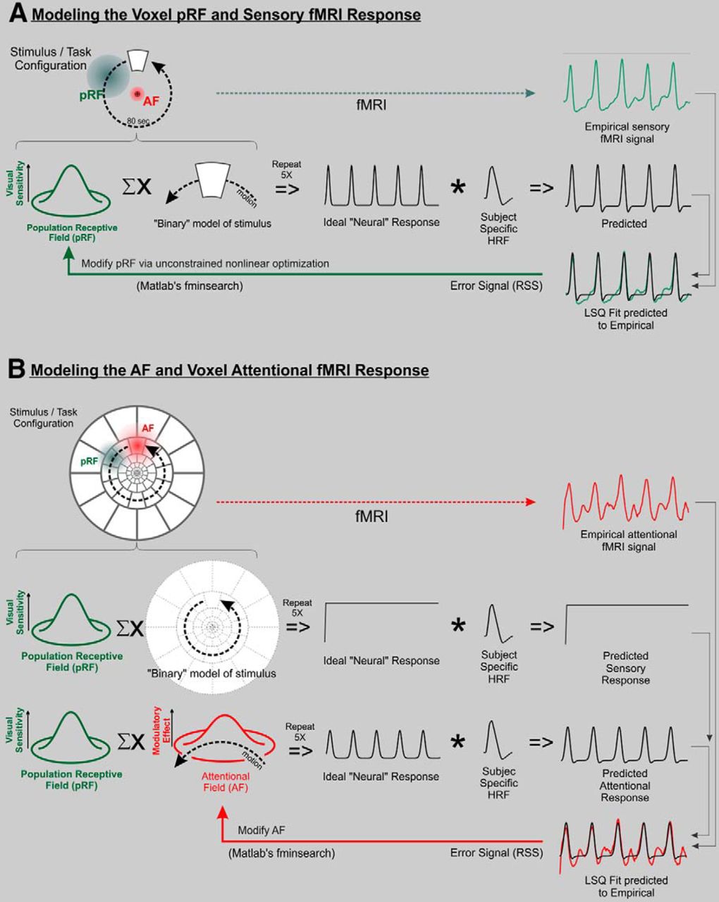
Schematic of single-voxel time-course modeling procedure for pRFs (A) and AFs (B). The procedures are based on the iterative optimization of either the pRF or AF to minimize the error between a computationally predicted response and an empirically sampled response. The combined ΣX symbol represents the spatial multiplication of the two patterns (either the pRF and stimulus or the pRF and AF) followed by integration over 2D space. This is repeated for each time point to yield the Ideal “Neural” Response. This Ideal “Neural” Response is then temporally convolved with a subject-specific HRF to generate the predicted fMRI response (see text for additional details on the modeling procedure).
The modeling procedure began with estimation of a voxel's pRF (Fig. 3A), which was modeled as a simple, 2D Gaussian distribution defined as follows:
 where (x0, y0) is the center position and σ is the standard deviation (SD) or spread of the distribution. The pRF was estimated using the fMRI response to the phase-encoded retinotopy stimuli acquired while the subject passively fixated the center of the display (note that any sensory stimulus can be used as long as its spatial distribution and motion is known; Fig. 3A illustrates the concept using the single target, sensory condition stimulus). An initial pRF estimate was multiplied with the spatial pattern of the stimulus and integrated over space to generate each successive time point of an Ideal “Neural” Response. A temporal convolution was then performed between the ideal response and the subject-specific HRF estimate (see below, Subject-specific HRF estimation) to generate a predicted fMRI response. An error signal was then computed as the residual sum of squared deviations (RSS) between the predicted response and the empirical response. The RSS error signal drove an iterative procedure that adjusted the location (x0, y0) and/or size (σ) of the pRF until an optimal fit between the predicted and empirical time courses was found. The expanding ring data were used to estimate the pRF eccentricity and the rotating wedge data were used to estimate the pRF angular position and size. The optimization procedure was performed in a two-pass, coarse-to-fine fashion and used an unconstrained nonlinear optimization algorithm (MATLAB's fminsearch algorithm). After each iteration of the optimization, an overall multiplicative scale factor and DC offset were used to obtain an optimal fit to the empirical time course (least-squared error best fit).
Once the pRF for a voxel had been estimated, a similar procedure (Fig. 3B) was performed to estimate the AF using the empirical fMRI time course evoked by the attention task. In this case, though, the AF itself was treated as a “virtual stimulus,” which moved across the pRF as dictated by the attention task. Since the stimulus array for the attention condition was comprised of nearly contiguous segments filling the display, the sensory response was modeled as an initial transient (at stimulus onset) followed by a sustained, unmodulated signal (Fig. 3B, Predicted Sensory Response). Concurrently, the response to the moving AF was modeled as a Gaussian (or Difference of Gaussians, DOG) spatial profile and “drifted” across the pRF using the known trajectory of the cued stimulus segment. At each point in time, the AF position was updated and the voxel's response amplitude was computed by multiplying the AF and pRF spatial profiles (at their current locations) and then spatially summing (integrating) the result. Repeating this calculation for each time increment yielded an Ideal “Neural” Response waveform (Fig. 3B) that was then temporally convolved with the subject-specific HRF to generate a Predicted Attentional Response. The amplitude of this predicted attentional response was adjusted to fit the empirically measured fMRI response using a least-squares fitting procedure. The RSS between the predicted and empirical signals was then used as an error signal to drive an iterative optimization procedure (MATLAB's fminsearch algorithm) that incrementally adjusted the AF model parameters to minimize the error between the predicted and empirical attention signals.
The AF was modeled twice, using a 2D Gaussian (Eq. 1) and DOG:
 where (x0, y0) is the center position of the DOG distribution, A is an amplitude scaling factor, σ1 is the SD of the first Gaussian, and σ2 is the SD of the second Gaussian. For the Gaussian model, the fitting procedure optimized the size and position of the AF, whereas for the DOG model the fitting procedure optimized these parameters as well as the size of the suppressive Gaussian and the relative amplitude of the two Gaussians.
To further elaborate, during the pRF modeling procedure (Fig. 3A) the spatial extent of the stimulus was known, the motion of the stimulus was known, and the spatial distribution of the pRF was unknown and thus was determined by the modeling procedure. In the AF modeling procedure (Fig. 3B) the spatial extent of the pRF is known (previously estimated; Fig. 3A), the motion of the AF is known, and the spatial distribution of the AF was unknown and thus determined by the modeling procedure. Unlike some previous studies (Womelsdorf et al., 2008; Klein et al., 2014), we assume that a voxel's total response reflects the combined effects of the sensory stimulation of a fixed pRF and its spatiotemporal modulation by the AF which, depending on the relative positions of the pRF and AF, can make it appear as if the pRF itself has changed (Moran and Desimone, 1985). In the account proposed here, the apparent pRF malleability is ascribed to the interaction of the pRF and AF rather than to the pRF itself. It is important to note that the method used here requires that a pRF be first estimated in a condition without attention, and then this estimate is used as the fixed pRF for estimating the AF. Although attention is still present, we measure the pRF using retinotopy acquired while the subject passively fixates the center of the display (no explicit attention condition) as a practical approximation of the fixed pRF.
Subject-specific HRF estimation.
Dumoulin and Wandell (2008) have emphasized that the BOLD HRF is “the most important non-neural influence on the pRF size estimate” when using a single-voxel time-course modeling approach. Moreover, HRFs have been shown to vary considerably across subjects (Kim et al., 1997; Aguirre et al., 1998; Handwerker et al., 2004). Consequently, HRFs were measured for each voxel using the response to a brief, large-field, flickering checkerboard as previously reported (Puckett et al., 2014). Subject-specific HRFs were then generated by averaging across all visual areas for each subject individually. These HRFs were then used as part of the time-course modeling procedures to estimate both the pRFs and AFs individually for each subject.
Suppressive surround index.
The suppressive surround index (SSI) was developed to help identify attention-related ADD responses better characterized by modeling the AF with a center surround distribution rather than a simple excitatory Gaussian. These voxels exhibit responses in which the peaks are flanked by regions of signal depression ostensibly caused by the presence of a suppressive surround associated with the AF. The SSI value quantifies the degree of this effect and is calculated by computing the Fourier magnitude spectrum of the response time course and then taking the ratio of the magnitudes of the second harmonic and fundament frequency components. The SSI tends toward zero for responses lacking regions of signal depression and increases as the surround effects become larger.
Voxel selection.
The pRFs were estimated for all voxels that were activated by both retinotopic stimuli and the single segment sensory localizer. The responses to each of these stimuli were subjected to a delay analysis using AFNI's Hilbert Delay plugin. Voxels with FDR-corrected, statistically significant correlation coefficients (q < = 0.001) were considered active. For the AF modeling procedure, only voxels with pRF centers between 1.5 and 6.5° or between 4 and 12° were used for the data collected at 4 and 8°, respectively (isolated based on their eccentricity estimates from the pRF modeling). This helped ensure that only voxels with pRFs that significantly intersected the AF trajectory were used to compute the AF. In addition, voxels with fMRI responses to the attention condition having low SNR (<0.5) and poor fits (correlation coefficient between the empirical fMRI response and the predicted response <0.4) were removed before further analyses.
Analysis of pRF size, AF size, AF surround size, and AF scatter.
The output parameters from the single-voxel time-course modeling procedures were used to estimate and quantitatively compare the relative sizes of the pRFs and AFs across the nine visual area ROIs. The sizes are reported in terms of the radius of the respective profiles. For Gaussian-modeled pRFs and AFs this corresponds to the half-width at half maximum. For the DOG-modeled AF, this corresponds to the half-width at the midpoint between the trough minimum and peak maximum. For the DOG-modeled AF, the surround size was estimated as the distance between the peak and the trough of the DOG profile. The parameters for all voxels in each ROI were averaged on an individual subject basis, and group analyses were performed on these averages. AF scatter was estimated by calculating the SD of the distribution of the AF angular position parameter.
AF model comparison metric.
The relative quality of the Gaussian and DOG AF models was assessed using Akaike's information criterion (AIC), which rewards a model based on goodness of fit but penalizes based on the number of estimated parameters (Akaike, 1974). AIC values were calculated for each model from single-voxel data using the following formula:
 where n is the number of data points in the voxel time course, RSS is the residual sum of squares from the modeling procedure, and p is the number of model parameters estimated (Burnham and Anderson, 2002). Importantly, there were two more parameters estimated when using the DOG model compared with the Gaussian (size of the second Gaussian and relative amplitude of the two Gaussians). AIC differences (ΔAIC) were then calculated for both models:
 where i denotes the model being assessed (Gaussian or DOG) and AICmin is the minimum AIC value within the set of models tested (in this case between the two models). The model estimated to best account for the data has AICi = AICmin and therefore ΔAICi = 0 (Burnham and Anderson, 2002).
Results
Subjects fixated a marker at the center of a rotating array of segments with constantly changing colors/orientations while covertly attending to and tracking a single target segment within the array (Fig. 1A). As a control, the subject alternately performed the same task but attended to a target segment behind the fixation marker (Fig. 1B). Finally, in a sensory condition, the subject attended to the center segment, but the previously attended peripheral segment was presented alone in the periphery (Fig. 1C). Statistical parametric activation maps and representative single-voxel time courses for each of these conditions are shown in Figure 4. Both the attention and sensory conditions elicited strong, retinotopically appropriate activation that was time locked to the rotational period of the stimulus array in each visual area ROI (Fig. 4A,C). Figure 4B shows that during the control condition when attention was directed to the demanding feature conjunction task at the fixation point, the stimulus array did not elicit a response modulated by the rotational period of the array, thus demonstrating that the signals in Figure 4A were related to attentional tracking of the target. Note that the onset of the stimulus array in Figure 4B did elicit an initial transient, but this was followed only by sustained activation without modulation timed to the array rotation. In the single target, sensory condition (Fig. 4C) attention was captured by the demanding task at fixation, away from the target. Therefore, the modulated response was due to the sensory effects of the isolated segment. In support of this interpretation, the behavioral response data (Table 1) show that all subjects performed the feature conjunction task well at the center segment during the single target condition and at the peripheral target location during the attention conditions. This verifies that subjects were consistently attending to the appropriate target in each condition, since feature conjunctions require attentional scrutiny to be reported accurately (Treisman and Gelade, 1980).

Stimulus/task (left) and cortical parametric flat maps (right) showing activation for attention (A), control (B), and sensory conditions (C). Dashed white line on cortical maps denotes 8° iso-eccentricity contour. Maps were FDR corrected and thresholded at q < 0.001. Raw data were smoothed with a 3.5 mm spherical kernel before correlation analysis. An example of a single-voxel response elicited by each condition is also shown from a voxel with a pRF lying along the target track. Data are from Subject 3. For visual area definitions see Figure 2.
Individual subject behavioral response data for feature conjunction task
Together, these results demonstrate how the task design permits isolation of attention-related modulation from sustained activation evoked by the stimulus array itself. In other words, from a sensory standpoint there is nothing unique about any particular segment in the array except when attention is directed to it. So in the attention condition (Fig. 4A), the phasic response must reflect the effects of attention.
Estimation of pRF and AF properties
We first estimated the pRFs using the single-voxel time-course modeling procedure (Fig. 3A). We were able to successfully model the sensory responses to both retinotopic stimuli (Fig. 5) in each visual area ROI. After obtaining the pRF estimates, we then successfully modeled attention signals (Fig. 3B) in each visual area for all subjects at 4° eccentricity. At 8° eccentricity we were able to model responses in all areas for each subject except for area V4 in a single subject and area LO in a different subject.

Subject 1 single-voxel responses (gray) and associated model fits (black) from the retinotopic stimuli across visual areas. Correlation coefficients (r) between responses and fits are also included. Left, Responses to rotating wedge stimulus. Right, Responses to expanding ring stimulus. The pRF was modeled by a Gaussian distribution.
Gaussian versus DOG AF models
Examples of single-voxel attention-related responses along with their model fits are shown in Figures 6 and 7. Inspection of the attention-related responses revealed that many voxels exhibited a response in which the signal peaks were flanked by regions of apparent signal depression (Fig. 6, areas V1, V2, and V3; Fig. 7, areas V1, V2, V3, V4, and V3AB). Such depressed sidebands can be taken into account by modeling the AF with a center-surround, DOG profile rather than a simple excitatory Gaussian. The DOG effectively incorporates a suppressive zone around the excitatory center region of the AF. This suppressive surround causes the signal to decrease as the AF first enters the voxel's pRF and again as it exits. As it moves further away from the pRF along the attention track, the signal begins to approach baseline when it is 180° away from the pRF. In addition to being able to qualitatively account for the depressed sidebands visible in the responses, the DOG model produces higher fit coefficients and lower AIC differences when fitting the responses with flanking regions of signal depression compared with the Gaussian model (Figs. 6, 7) suggesting that the DOG is a more appropriate AF model than the simple Gaussian.

Subject 1 single-voxel responses (gray) and associated model fits (black) from the attention condition of the ADD experiment performed at 8° eccentricity. Left, Gaussian model. Right, DOG model. AIC differences (ΔAIC) for each AF model and correlation coefficients between responses and fits (r) are also included. Responses were taken from the same voxels as in Fig. 5.

Subject 3 single-voxel responses (gray) and associated model fits (black) from the attention condition of the ADD experiment performed at 8° eccentricity. Left, Gaussian model. Right, DOG model. AIC differences (ΔAIC) for each AF model and correlation coefficients between responses and fits (r) are also included. Note: This subject lacked significant responses in area LO.
One potential concern is that sensory pRFs have been shown to exhibit DOG profiles in some visual areas (Zuiderbaan et al., 2012). This raises the question of whether the surround effects we have ascribed to the AF are actually a reflection of pRF suppressive surrounds. However, this type of response was distinct from those elicited by the single target sensory condition (Fig. 8) and retinotopic stimuli (Fig. 5). Close examination of the time courses of individual voxels to the attention condition (Fig. 8) clearly shows the presence of depressed “troughs” before and after the positive peak in the attention responses (particularly prominent for V2, V3, V4, and V3AB). Yet, this is not apparent in the single-segment sensory responses as would be expected if the pRF itself had a DOG sensitivity profile.

Single-voxel responses to both the attention and sensory conditions of the ADD experiment performed at 8° eccentricity for Subject 3. Responses were taken from the same voxels as in Fig. 7. Note the lack of secondary peaks in sensory responses.
An SSI was used to identify responses showing strong suppressive effects, and the group-averaged SSI values were plotted as a function of visual area to investigate the cortical distribution of these responses (Fig. 9). As shown in Figure 9, these responses are most prominent in lower order visual areas and become less prominent at higher levels of the visual hierarchy. As expected, this precisely corresponds with what is seen in the single-voxel time courses, particularly those in Figure 7.

Group-average SSIs associated with the DOG AF model fits across visual areas. Error bars represent ± SEM.
The lack of flanking regions of signal depression in the attention responses of higher order areas does not necessarily preclude the AF from having a suppressive surround in those areas. Instead the observed results may be a consequence of the experimental design and the relative sizes of the pRFs and AFs across the cortical hierarchy. In visual areas with large AFs, a voxel's pRF may never completely escape the suppressive effects of attention except when the positive peak of the AF crosses it. Thus, the seemingly disparate attentional effects across visual areas may simply reflect quantitative differences arising from the interplay of pRF and AF sizes across the visual hierarchy rather than result from fundamental differences in the neurophysiology of attention across visual areas. To investigate this possibility we computed group-averaged estimates of the size of the AF suppressive surround and plotted them across visual areas (Fig. 10, right). Comparing Figure 10 with Figure 9 shows that the group-averaged AF surround sizes were negatively correlated with the SSI at both 4 and 8° eccentricities across visual areas (r = −0.85, −0.95, respectively). This lends support to the notion that as the suppressive surrounds becomes larger the presence of flanking regions of signal depression in the responses to the ADD experiment diminish, presumably due to the suppressive surrounds being too large to sufficiently exit the pRF thereby preventing the response from returning to baseline. In addition, lower AIC differences were associated with the DOG model compared with the Gaussian model for each time course fit in Figures 6 and 7 suggesting that the DOG is a more appropriate AF model than the Gaussian, even when there is no clear flanking region of signal depression.

Comparison of group-averaged pRF and AF sizes across visual areas for both AF models (left, Gaussian; right, DOG) and both eccentricities. See schematics (top) for size definitions: for the Gaussian AF the size is the radius of the center peak at half maximum (Rc), for the DOG AF the size is the radius of the center peak at half maximum (Rc), and the AF surround size is the radius from the center of the peak to the minimum of the suppressive trough (Rs). For all pRFs the size is the radius of the center peak at half maximum (Rc). Black dashed lines across the bar graphs represent the full width of the attended target (W).
It is important to note that the experiment reported here was designed to explicitly measure the spatial extent of the AF in the circumferential direction along the track of the attended target. We modeled the AF as a symmetrical distribution using this measurement, but this may not be the case. Contrasting the cortical activation maps between the attention (Fig. 4A) and sensory (Fig. 4C) conditions reveals attentional activation extending beyond the range of eccentricities activated by the single target. The attentional activation, while strongest at the target eccentricity, extends inward across more foveal locations suggesting that the AF may have an asymmetric distribution across visual field eccentricity consistent with previous reports (Brefczynski-Lewis et al., 2009; Datta and DeYoe, 2009; Simola et al., 2009) and with behavioral evidence (Downing and Pinker, 1985). To investigate this issue in more detail, the attentional drift design described here can be extended by drifting the attended target inward/outward to explore AF topography along the radial dimension as well.
AF versus pRF size
For both Gaussian and DOG AF models we computed and compared the group-averaged AF sizes with the pRF sizes across the visual area ROIs (Fig. 10). These measurements were also used to illustrate the sizes of the pRFs and AFs relative to the stimulus array/target at both eccentricities (Fig. 11). Inspection of the pRF sizes reveals that the pRFs scale in size across eccentricity and vary across visual area as expected. The absolute sizes of the pRFs are in close correspondence with those previously reported for lower visual areas (V1, V2, and V3) but appear smaller in higher areas such as V4 and LO (Dumoulin and Wandell, 2008; Harvey and Dumoulin, 2011). Like the pRFs, we also found that the AFs scale in size with eccentricity and vary across visual areas (Figs. 10, 11).
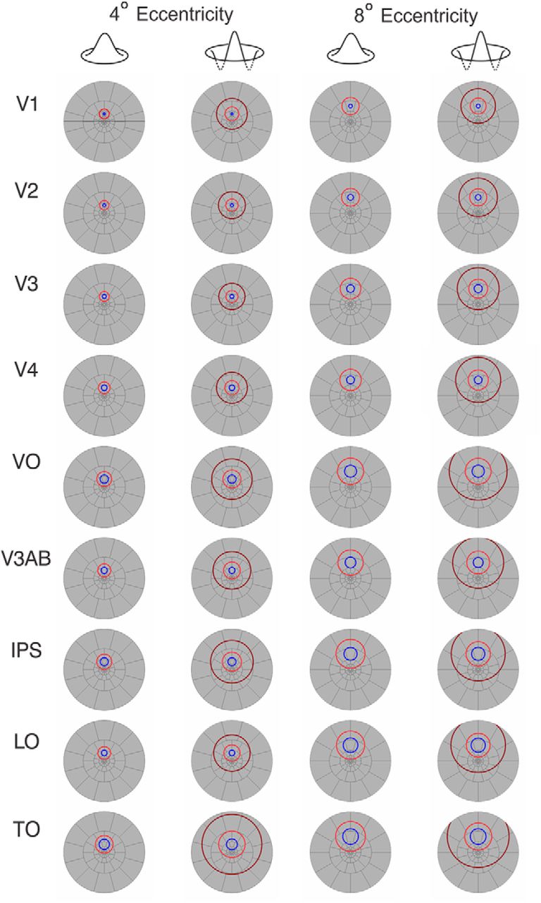
Illustrative comparison of stimulus size to group-averaged pRF and AF sizes across visual areas for both AF models and both eccentricities. Blue line, pRF size; bright red line, AF size; dark red line, AF suppressive surround size.
It is important to stress that the AF measurements obtained in the experiment reported here were constrained by the segment spacing of the stimulus array, which was intentionally adjusted to be at the perceptual “crowding limit” (Intriligator and Cavanagh, 2001). While it is not clear whether this limit is set by the size of the attentional field or other factors (Intriligator and Cavanagh, 2001; Pelli and Tillman, 2008), it is nevertheless arguable that under these conditions, the focus of attention must be well controlled to include the attended target while excluding neighboring distracter information. In other words, correct reporting of the target features likely depends on the target spacing being large enough to avoid “crowding” but also on having the attentional field small enough to exclude distracters. Indeed, the sizes of the AFs measured here were in close correspondence with the sizes of the attended targets, particularly in lower order visual areas (Figs. 10, 11). However, since crowding effects are known to scale with eccentricity, the spacing of the segments must also scale with eccentricity, and to maintain stimulus continuity (avoiding blank areas between segments), they must also scale in size. Therefore, the stimulus design unavoidably confounds target size, spacing, and eccentricity. So, it remains unclear which factor (or factors) ultimately set the AF size. Future experiments could explore the ability of the AF to adjust in size and topography under more varied task conditions. This could include expansion of the field to include multiple neighboring segments or to assume a more irregular shape as has been explored previously using behavioral methods (Gobell et al., 2004). It could also be used to explore the topography of the attentional field under conditions requiring attention to multiple targets separated by distractors (McMains and Somers, 2004; Morawetz et al., 2007).
AF scatter
As part of the modeling procedure, we allowed the AF angular position to be optimized, thereby enabling the AF to be offset from the center of the attended target. Indeed, the quantitative analysis showed that the fMRI responses were better fit by allowing this offset. Theoretically, one might have anticipated that there could be a consistent offset if the voluntary shifting of the AF was lagging behind the target array rotation. However, the distribution of the AF offsets was symmetric with approximately equivalent numbers of both leading and lagging offsets (Fig. 12). While such an offset scatter might seem peculiar, it is important to point out that to perform the task accurately subjects only need to attentionally isolate a portion of the target since the color/orientation pattern extends throughout its width.

Histograms of attentional field scatter for both AF models (left, Gaussian; right, DOG) and both eccentricities. Mean (x̄) and SD (σ) of the distributions are also included.
Discussion
This study demonstrates a new, fMRI-based technique to quantitatively measure the topography of spatial attention from single brain voxels using a time-course modeling procedure. The results show that when subjects attend to single targets within a crowded array, retinotopically appropriate attentional modulation of neuronal activity occurs throughout cortical visual areas: V1, V2, V3, V4, VO-1,2, V3AB, IPS-0,1,2,3, LO-1,2, and TO-1,2. The spatial extent of the attentional field scales with eccentricity for targets at 4° and 8°. Under our test conditions, the attentional field typically features a suppressive surround that is not a reflection of the structure of the sensory receptive field. Use of these data in conjunction with existing and future neurophysiological models of attention should help elucidate the operation of attention within each visual area and clarify how the individual effects separately and collectively account for the perceptual features of spatial attention.
The ADD method
The attentional drift design reported here provides a way to use single-voxel time-course modeling to quantitatively measure the cortical effects of attention in human subjects. This approach avoids or minimizes many of the limitations associated with a previous method in which we attempted to reconstruct the attentional field topography from multiple voxels recorded simultaneously within each cortical area (Puckett et al., 2010). Such limitations included susceptibility artifacts, coarse voxel sampling, and uncontrolled variations in response magnitude from voxel to voxel. These limitations were exaggerated in higher order visual areas composed of few voxels and hampered efforts to make detailed measurements of the topography of attention in later stage visual areas. By avoiding these limitations, detailed measurements of attentional field topography were obtained throughout the cortical hierarchy of visual areas. Moreover, this method can reveal complex topographical features of the AF, such as a suppressive surround, thereby making it particularly well suited for exploring and modeling the interactions among visual stimuli, sensory receptive fields, attentional fields, and behavioral task requirements.
Klein et al. (2014) recently published a similar method to estimate the size of the AF from single-voxel responses throughout visual cortex. Their method, however, relies on indirectly estimating the size of the AF from attention-induced changes in the “pRF preferred positions,” whereas we were able to measure the AF more directly by drifting the AF though the pRF under constant sensory stimulation. This difference in methodology is accompanied by an important conceptual difference. It is our position that attention does not actually alter a neuron's RF size or location. Rather, apparent RF/pRF changes, such as those reported previously (Womelsdorf et al., 2008; de Haas et al., 2014; Klein et al., 2014), reflect the combined interaction of the sensory stimulus, a fixed RF/pRF, and the attentional modulation (as modeled by the AF). Note that in the seminal article by Moran and Desimone (1985) on the effects of attention on single neuron responses, they carefully stated that it was “almost as if the receptive field had contracted around the attended stimulus.” Though others acknowledge this potential reservation, it nevertheless has become popular to describe the attentional effects as altering the RF/pRF itself.
Attentional fields
Topography of attentional effects
The notion that the phenomenological effects of attention are spatially distributed as an extended topography has been a consistent theme going back at least as far as James (1890), von Helmholtz (1909), and Wundt (1924/1896). In more recent times, detailed knowledge of multiple hierarchically organized visual areas (Felleman and Van Essen, 1991) and the ubiquity of attentional effects throughout visual cortex (Kastner et al., 1998; Tootell et al., 1998; Brefczynski and DeYoe, 1999; Brefczynski-Lewis et al., 2009) have begun to make it clear that the phenomenal effects of attention, including its perceptual topography, likely arise from the aggregate operation of multiple neurophysiological representations of the “window” of attention. For this reason, it is clear that no theory of visual attention will be complete unless it accounts for the working of attention in each visual area. Yet, detailed empirical data specifying the precise topography of each of these neuronal attentional fields has been lacking, especially in humans. Accordingly, it is not surprising that there have been relatively few theoretical models that have incorporated such multiple, hierarchical AFs into a comprehensive, mechanistic account of how attention operates within the brain. Notable exceptions have been some of the hierarchical concepts associated with the Feature Integration theory (Treisman and Gelade, 1980), the Neural Theory of Visual Attention (Bundesen et al., 2005), and the Selective Tuning model (Tsotsos, 2011). The data and models of the AFs described here should help remedy this situation and stimulate further development along these lines.
Suppressive effects
We demonstrated attention-related time-course responses from a number of visual areas that provide clear evidence that the AF has flanking suppressive effects that we have modeled here as a suppressive surround. Suppressive effects are consistent with many previous behavioral and neurophysiological studies of attention (Lee et al., 1999; Müller and Kleinschmidt, 2004; Müller et al., 2005; Silver et al., 2007; Sylvester et al., 2008; Boehler et al., 2009; Boynton, 2009; Reynolds and Heeger, 2009; Carrasco, 2011; Tsotsos, 2011). However, the data and model presented here are primarily intended to be descriptive rather than represent a strong statement concerning which of several neural mechanisms might be responsible for these suppressive effects. For instance, biased competition models of attention largely ascribe suppressive effects to lateral interactions among the sensory representations of locally competing stimuli (Desimone and Duncan, 1995; Desimone, 1998). In such models, attention simply enhances or “disinhibits” the response of the attended target allowing it to win the local competition and suppress nearby unattended distractors (Desimone, 1998). The attention-related fMRI responses we report here could be consistent with such a scenario. Another potential interpretation is that the effects that we have here described as suppressive, meaning simply a reduced signal, might reflect a spatial normalization mechanism akin to that described previously (Reynolds and Heeger, 2009; Lee and Maunsell, 2009). Lacking more definitive data at this time, we have provisionally ascribed the suppressive effects we observed empirically to the operation of a DOG attentional field topography that is relatively simple to model and accounts for our data. Future work will be needed to clarify the true nature of the underlying neural mechanism and whether the suppressive effects are part of the modulatory signals that constitute the neuronal representation of the AF or arise from interactions between the attention signals and the cortical circuitry upon which they operate.
AF scatter
One unexpected result of the AF modeling was that offsets between the AF and the center of the attended target were required to model the time-course data most accurately. These parameters represent voxelwise offsets between the centers of the AF and the attended target. The population distribution of these offsets (Fig. 12) was symmetric in both directions, “leading” and “lagging” the target position. This symmetry argues against a behavioral “lag” in keeping the focus of attention updated with the target motion, which was quite slow to begin with. We propose that the distribution of AF angular offsets may represent the spatial scatter associated with attempting to maintain attention on a single target within the array, a concept akin to the scatter produced by microsaccades during eye gaze fixation but on a slower timescale. We speculate that the offset for an individual voxel represents an average of the random moment-to-moment variation in the location of the attentional focus for the 25 times that the AF passed over the pRF (5 cycles per scan × 5 scans). For the majority of voxels, the offset was <30 degrees of rotation, which is equivalent to the segment-to-segment spacing in the target array. One might wonder if subjects often “lost track” of the cued target and unknowingly shifted attention to one of its neighbors. However, the use of brief “reminder” cues (see Materials and Methods) helped to minimize this possibility and such shifts would have been easily identified in the button performance records as a failure to correctly report the target features. In fact, performance was uniformly high and as good as when constantly attending to the center target (Table 1). Other possible contributions could be random variations in the hemodynamic response of individual voxels and errors in the estimation of pRF locations.
Implications for models of attention
The spatial topography of attention is a distinguishing feature in a variety of theoretical models of visuospatial attention (Posner et al., 1980; Downing and Pinker, 1985; Eriksen and St James, 1986; Sperling and Weichselgartner, 1995; Dosher et al., 2004; Boehler et al., 2009; Reynolds and Heeger, 2009). The attentional drift task design and AF modeling technique reported here provides a source of data to be used in constraining and testing such models. Of particular interest in this respect is the normalization model of visual attention described previously (Reynolds and Heeger, 2009). This model suggests that seemingly distinct modulatory effects attributed to attention such as contrast-gain versus response-gain (Williford and Maunsell, 2006; Lee and Maunsell, 2010) can be unified under a single computational framework in which the sensory pRF and the AF are independently modeled (along with a divisive normalization field). The critical factors that determine what type of modulation occurs are the spatial extent of the distribution of attentional effects, the pRF, and the attended stimulus. By providing empirical measurements of both the pRF and AF characteristics, the attentional drift paradigm described here provides important data for testing such models and, ultimately, creating a comprehensive neurophysiological account of the perceptual effects of visuospatial attention.
Footnotes
This research was supported by National Institutes of Health Grants R01EB000843 to E.A.D. and R01EB007827 to J. Hyde. We thank Jed Mathis and Yan Ma for technical contributions and Andy Salzwedel for helpful discussions.
The authors declare no competing financial interests.
- Correspondence should be addressed to Alexander M. Puckett, University of Wollongong–School of Psychology, Northfields Avenue, Wollongong, NSW 2522, Australia. pucketta{at}alumni.msoe.edu


