
Abstract
In nonhuman primates (NHPs), secondary visual cortex (V2) is composed of repeating columnar stripes, which are evident in histological variations of cytochrome oxidase (CO) levels. Distinctive “thin” and “thick” stripes of dark CO staining reportedly respond selectively to stimulus variations in color and binocular disparity, respectively. Here, we first tested whether similar color-selective or disparity-selective stripes exist in human V2. If so, available evidence predicts that such stripes should (1) radiate “outward” from the V1–V2 border, (2) interdigitate, (3) differ from each other in both thickness and length, (4) be spaced ∼3.5–4 mm apart (center-to-center), and, perhaps, (5) have segregated functional connections. Second, we tested whether analogous segregated columns exist in a “next-higher” tier area, V3. To answer these questions, we used high-resolution fMRI (1 × 1 × 1 mm3) at high field (7 T), presenting color-selective or disparity-selective stimuli, plus extensive signal averaging across multiple scan sessions and cortical surface-based analysis. All hypotheses were confirmed. V2 stripes and V3 columns were reliably localized in all subjects. The two stripe/column types were largely interdigitated (e.g., nonoverlapping) in both V2 and V3. Color-selective stripes differed from disparity-selective stripes in both width (thickness) and length. Analysis of resting-state functional connections (eyes closed) showed a stronger correlation between functionally alike (compared with functionally unlike) stripes/columns in V2 and V3. These results revealed a fine-scale segregation of color-selective or disparity-selective streams within human areas V2 and V3. Together with prior evidence from NHPs, this suggests that two parallel processing streams extend from visual subcortical regions through V1, V2, and V3.
SIGNIFICANCE STATEMENT In current textbooks and reviews, diagrams of cortical visual processing highlight two distinct neural-processing streams within the first and second cortical areas in monkeys. Two major streams consist of segregated cortical columns that are selectively activated by either color or ocular interactions. Because such cortical columns are so small, they were not revealed previously by conventional imaging techniques in humans. Here we demonstrate that such segregated columnar systems exist in humans. We find that, in humans, color versus binocular disparity columns extend one full area further, into the third visual area. Our approach can be extended to reveal and study additional types of columns in human cortex, perhaps including columns underlying more cognitive functions.
- high-resolution fMRI
- stereoscopic depth
- streams
- stripes
- visual features
Introduction
In visual cortex of nonhuman primates (NHPs), different stimulus features are processed in correspondingly different “streams,” organized partly in functionally segregated columns. Analysis of such cortical columns reveals the basic “functional tasks executed by any given area” (Mountcastle, 1997). Such streams are especially prominent in “stripe”-shaped columns within area V2 (i.e., the earliest stage of extrastriate visual cortex). However, it is unknown whether a comparable columnar organization exists in humans.
V2 stripes
In NHPs, V2 stripes radiate perpendicularly from the V1–V2 border in the cortical map (Fig. 1; Livingstone and Hubel, 1982; Tootell et al., 1983). These V2 stripes are columns in the broadest sense, because they express a regular and repeating variation in function, spanning most or all of the cortical layers, throughout V2.

Histological tissue section showing varying levels (darker = higher) of the metabolic enzyme CO, in flattened visual cortex in the right hemisphere of a monkey (Saimiri sciureus). The discrete darkly stained region on the left is V1. Immediately anterior (to the right) is area V2, including layers 4 and 5. The darkly stained CO stripes in V2 are subdivided into thin (thin red triangles) and thick (wider green triangles). The thin stripes extend contiguously to the V1–V2 border; the thick stripes terminate slightly shy of the V1–V2 border. Scale bar, 2 mm. Figure adapted from Tootell et al., 1983.
V2 stripes are typically defined based on distinctive histological variations in cytochrome oxidase (CO) activity. Repeating units are composed of a “thin” dark (high CO) stripe, flanked by two “pale” (low CO) stripes, plus a “thick” dark stripe (Livingstone and Hubel, 1982; Tootell et al., 1983). In NHPs, the thin stripes show high sensitivity to variations in stimulus color, relative to luminance (Tootell et al., 1983, 2004; Hubel and Livingstone, 1985; 1987; Roe and Ts'o, 1995; Xiao et al., 2003). In contrast, thick stripes show selectivity for a quite different visual feature, binocular disparity (Hubel and Livingstone, 1987; Peterhans and von der Heydt, 1993; Chen et al., 2008).
Homologous stripes may exist in human V2, based on histological staining for CO (Tootell and Taylor, 1995; Adams et al., 2007), myelin (Tootell and Taylor, 1995), or CAT-301 (Hockfield et al., 1990). However, such histological observations are quite limited.
It has been speculated that the columnar segregation of color versus disparity processing in macaque V2 is related to an analogous segregation of color and disparity processing in human perception (Livingstone and Hubel, 1987; Cavanagh and Leclerc, 1989). Although this remains an intriguing possibility, such functional properties cannot be concluded directly from the available evidence, based on either the postmortem histological studies in humans or neurophysiological studies in anesthetized NHPs. Accordingly, one goal of the present study was to test for color-selective or disparity-selective stripes in awake human V2, using high-resolution fMRI.
Related columns in area V3?
In humans and macaques, area V3 is located immediately anterior to V2. In macaques, V3 receives direct input from both V1 and V2 (Felleman and Van Essen, 1991), two areas in which cortical columns are well known. Despite this, little is known about the possible existence (and nature) of columns in V3, in any primate species.
Unfortunately, it is challenging to resolve the columnar organization in V3 based on experiments in NHPs. For instance, V3 in humans differs retinotopically from V3 in different species of NHP. In macaques, neurobiological experiments can be challenging because V3 is quite thin in the cortical map and is buried within deep sulci (Felleman and Van Essen, 1991).
In contrast, the surface area of V3 is greatly expanded in the human cortical map, compared with macaque (Sereno et al., 1995; Tootell et al., 1997). In humans, V3 is approximately as large as V2 (Sereno et al., 1995; Tootell et al., 1997), which implies that V3 plays a significant processing role in human visual cortical processing. In any event, the large size of human V3, coupled with the ability to visualize human columns with fMRI, offers an invaluable opportunity to test whether the elaborately segregated columnar organization in V2 extends further into an immediately higher level, V3. Thus, a second goal of this study was to test for color- versus disparity-selective columns in V3.
Materials and Methods
Participants
Eight human subjects (five females; age range, 24–35 years) participated in this study. All subjects had normal or corrected-to-normal visual acuity and radiologically normal brains, without history of neuropsychological disorder. All experimental procedures conformed to National Institutes of Health (NIH) guidelines and were conducted according to Massachusetts General Hospital protocols. Written informed consent was obtained from all subjects before the experiments.
General procedures
Each subject was scanned multiple times (over different days) in a high-field scanner (7 T whole-body system, Siemens Healthcare) to localize color-selective stripes/columns (two sessions) and to study their functional connections (one session). Six of eight subjects (three females) also participated in a second experiment, which localized disparity-selective stripes/columns and tested for ocular interactions (two to three additional sessions). The sequence of experiments was counterbalanced between the subjects. In addition, all eight subjects were scanned in a 3 T scanner (Tim Trio, Siemens Healthcare) in one separate session for structural and retinotopic mapping (one session).
Visual stimuli
Stimuli were presented via an LCD projector (1024 × 768 pixel resolution, 60 Hz refresh rate) onto a rear-projection screen, viewed through a mirror mounted on the receive coil array. Matlab 2013a (MathWorks) and the Psychophysics Toolbox (Brainard, 1997; Pelli, 1997) were used to control stimulus presentation.
During all experiments (except for resting-state scans), stimuli were presented in a blocked-design procedure. Subjects were required to fixate a small (0.1° × 0.1°) central fixation spot. To control their level of attention during the scans, subjects were required to report changes in the color of the fixation spot by pressing a key on a keypad (i.e., an unrelated, “dummy” attention task).
Experiment 1: color experiment.
Sinusoidal gratings (20° × 20° visual angle) were presented that varied in either color or achromatic luminance, presented in separate blocks. The color-varying gratings varied along an axis between the red and blue values of maximal purity for this display. For each subject, colors were adjusted to be equal in luminance across the range of eccentricities stimulated, according to each subject's color perception (see below). The spatial frequency of all gratings was low (0.2 cycle/°), to tap the relatively higher sensitivity to color (relative to luminance) at that spatial scale (van der Horst and Bouman, 1969; Granger and Heurtley, 1973) and to minimize linear chromatic aberration (i.e., luminance artifacts) at color borders.
During the scans, in different blocks, grating stimuli were presented at different orientations (either 0°, 45°, 90° or 135°), drifting in orthogonal directions (reversed every 6 s) at 4°/s. Each run started and finished with a short block (18 s) of uniform gray of equal mean luminance. Remaining blocks in each run included nine stimulus presentation blocks (24 s/block). Each subject participated in 12 runs/session, during which 1008 functional volumes were collected (see Imaging subsection below).
Luminance adjustment.
It is well known that the isoluminance ratio of color-varying stimuli varies with stimulus eccentricity (Mullen, 1985; Livingstone and Hubel, 1987; Bilodeau and Faubert, 1997). Therefore, for each subject, we adjusted the red/blue luminance ratio at three different eccentricity ranges (0–2°, 2–5°, and 5–10°) based on flicker photometry (Ives, 1907; Bone and Landrum, 2004). More specifically, immediately before the functional scans (inside the scanner), the subject viewed a spatially uniform blue (Fig. 2A) in temporal counterphase with gray, at 30 Hz. The luminance of the spatially uniform blue was set to the maximum (RGB: 0, 0, 255). We used blue in this comparison because it was the limiting (lowest) luminance among our color stimuli. Subjects increased and decreased the luminance of the gray image relative to the reference blue to minimize the perceived flicker (i.e., optimizing perceived fusion) by using two keys on a keypad. This process was repeated four times for each eccentricity. The sequence of presentation was pseudo-randomized to avoid multiple adjustment of the same eccentricity consecutively. Subsequently, the measured luminance (intensity) values were averaged independently for each eccentricity (Fig. 2B). Based on these measured gray luminance values, we repeated this process to find the isoluminance values for red, across the same eccentricities. This time, subjects had to minimize the perceived flicker (i.e., increased perceptual fusion) when gray values were presented (flickered) against red (Fig. 2C).
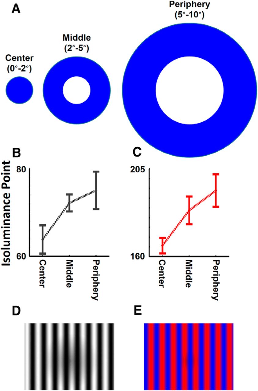
A, A sample of stimuli used for luminance adjustment across central (0–2°), middle (2–5°), and peripheral (5–10°) eccentricities. B, C, The measured level of luminance for gray (B) and red (C) colors that match the luminance of maximum blue values in the scanner display. D, E, Samples of achromatic (D) and chromatic (red/blue; E) stimuli. Error bars indicate 1 SEM.
Figure 2, B and C, respectively, show the measured luminance values of gray and red for the eight subjects who participated in Experiment 1. Each subject was scanned twice, and these values were measured independently in each session. Consistent with previous reports (Mullen, 1985; Livingstone and Hubel, 1987; Bilodeau and Faubert, 1997), we found a significant effect of eccentricity on the measured luminance of gray (F(2,30) = 3.88, p = 0.03) and red (F(2,30) = 17.07, p < 10−4).
The luminance values of red (measured across different eccentricities) were used to generate red/blue gratings. More specifically, while the blue intensity remained the same across the red/blue gratings, we adjusted the luminance of each red pixel according to its eccentricity, and a logarithmic function was fit to each subjects' own measured luminance values. Similarly, the luminance values for gray were also used to calculate the white point in the achromatic grating stimuli at different eccentricities. In this achromatic control stimulus, the luminance of the “black” nadir of the sinusoidal stripes was set to zero, and the luminance white pixels varied with eccentricity based on a logarithmic function fit to the subjects own measured luminance values. Samples of these red-blue grating stimuli and their achromatic control stimuli are shown in Figure 2D–E.
Experiment 2: disparity experiment.
Disparity-varying stimuli were sparse (5%) random dot stereograms (RDSs) based on red or green dots (0.09° × 0.09°) presented against a black background, extending 20° × 20° in the visual field. Subjects viewed the stimulus through custom anaglyph spectacles using Kodak Wratten filters No. 25 (red) and 44A (cyan). Two RDSs (each either red or green) were overlaid and fused within all experiment blocks. In one condition, stimuli formed a stereoscopic percept of a regular array of cuboids that varied sinusoidally in depth (±0.22°), with independent phase, similar to a stimulus described earlier (Tsao et al., 2003; Neri et al., 2004; Bridge and Parker, 2007; Minini et al., 2010). In the control condition, the fused percept formed a frontoparallel plane intersecting the fixation target (i.e., zero depth at that point). For a subset of subjects in this experiment (n = 4), we also presented analogous stimuli monocularly to either their left or right eye within separate blocks. These stimuli were perceived as moving dots at zero depth.
Each experimental run began and ended with 12 s of uniform gray (“blank”), and included eight stimulus blocks (24 s/block). Each subject participated in 12 runs/session, during which 864 functional volumes were collected.
Retinotopy mapping.
Details of retinotopic mapping have been reported previously (Nasr et al., 2011). Briefly, stimuli were colorful images of scenes and face mosaics, which were presented within retinotopically limited apertures, against a gray background. The retinotopic apertures included horizontal and vertical meridian wedges (radius, 10°; polar angle, 30°).
To reconfirm the V1/V2/V3 borders, in three subjects (Subjects 1, 2, and 5), we also used phase-encoded, contrast-reversing (1 Hz) checkerboards within continuously rotating rays or continuously expanding/contracting ring stimuli for retinotopy mapping. Details of this procedure were described previously (Sereno et al., 1995).
Imaging
7 T sessions.
Experiments 1–2 were conducted in a 7 T Siemens whole-body scanner equipped with SC72 body gradients (maximum gradient strength, 70 mT/m; maximum slew rate, 200 T/m/s) using a custom-built 32-channel helmet receive coil array and a birdcage volume transmit coil (Keil et al., 2010). Voxel dimensions were nominally 1.0 mm, isotropic, except as noted below. Single-shot gradient-echo EPI was used to acquire functional images with the following protocol parameter values: TR, 3000 ms; TE, 28 ms; flip angle, 78°; matrix, 192 × 192; band width (BW), 1184 Hz/pix; echo-spacing, 1 ms; 7/8 phase partial Fourier; FOV, 192 × 192 mm; 44 oblique-coronal slices; and acceleration factor r = 4 with GRAPPA reconstruction and FLEET-ACS data (Polimeni et al., 2015) with 10° flip angle. The field of view included occipital cortical areas V1, V2, V3, and the posterior parts of V4v and V4d.
For one subject, we also acquired functional images with higher resolution (0.8 mm, isotropic) with the following protocol parameter values: TR, 4000 ms; TE, 28 ms; flip angle, 78°; matrix, 192 × 192; BW, 1184 Hz/pix; echo-spacing, 1 ms; 7/8 phase partial Fourier; FOV, 153.6 × 153.6 mm; 54 oblique-coronal slices; and acceleration factor r = 4 with GRAPPA reconstruction and FLEET-ACS data with 10° flip angle.
During the resting-state scans, fMRI brain activity fluctuations were measured using a similar 1.0 mm isotropic EPI protocol but with a TR of 4000 ms, a flip angle of 85°, and 59 oblique-coronal slices. Here again, the field of view included areas V1, V2, V3, and the posterior parts of V4v and V4d.
Our voxel size estimation might be affected by pulsatility artifacts plus the draining vein effect of the underlying vasculature. We tried to minimize the latter impact of blurring due to the large vessels by differential stimulation paradigms (also see Yacoub et al., 2008), and also by sampling far from the pial surface (Polimeni et al., 2010; also see below). With regard to the former (pulsatility artifacts), previous studies (Enzmann and Pelc, 1992; Poncelet et al., 1992) have estimated this effect to produce ∼90 μm of tissue displacement in the occipital lobe of humans, in vivo, under normal physiological conditions. Therefore, it should not have a major impact on our measurements.
3 T sessions.
Retinotopy mapping was conducted using a 3 T Siemens scanner (Tim Trio) and the vendor-supplied 32-channel receive coil array. Functional data were acquired using single-shot gradient-echo EPI with nominally 3.0 mm isotropic voxels using the following protocol parameters: TR, 2000 ms; TE, 30 ms; flip angle, 90°; matrix, 64 × 64; BW, 2298 Hz/pix; echo-spacing, 0.5 ms; no partial Fourier; FOV, 192 × 192 mm; 33 axial slices covering the entire brain; and no acceleration.
Structural (anatomical) data were acquired using a 3D T1-weighted MPRAGE sequence with protocol parameter values: TR, 2530 ms; TE, 3.39 ms; TI, 1100 ms; flip angle, 7°; BW, 200 Hz/pix; echo spacing, 8.2 ms; voxel size, 1.0 × 1.0 × 1.33 mm; FOV, 256 × 256 × 170 mm.
General data analysis
Functional and anatomical MRI data were preprocessed and analyzed using FreeSurfer and FS-FAST [version 5.3 (http://surfer.nmr.mgh.harvard.edu/); Fischl, 2012]. For each subject, inflated and flattened cortical surfaces were reconstructed based on the high-resolution anatomical data (Dale et al., 1999; Fischl et al., 1999, 2002).
All functional images were corrected for motion artifacts. Three tesla functional data were spatially smoothed (Gaussian filtered with a 5 mm FWHM). However, no spatial smoothing was applied to the main imaging data acquired at 7 T (i.e., 0 mm FWHM). For each subject, functional data from each run were rigidly aligned (6 df) relative to his/her own structural scan using rigid Boundary-Based Registration (Greve and Fischl, 2009). This procedure enabled us to average data collected for each subject across multiple scan sessions.
A standard hemodynamic model based on a gamma function was fit to the fMRI signal to estimate the amplitude of the BOLD response. For each individual subject, the average BOLD response maps were calculated for each condition (Friston et al., 1999). Finally, voxelwise statistical tests were conducted by computing contrasts based on a univariate general linear model, and the resultant significance maps were projected onto the subject's anatomical volumes and reconstructed cortical surfaces.
Specific data analysis and tests for 7 T data.
To test for a columnar organization, we subdivided and compared fMRI activity from three cortical depths, as described previously (Polimeni et al., 2010). Briefly, for each subject the gray matter–white matter (deep) interface and the gray matter superficial (pial) surface were generated from their own high-resolution structural scans (see above) using FreeSurfer (Dale et al., 1999; Fischl et al., 1999, 2002). In addition to these two surfaces, an intermediate “mid-gray” surface was also generated at 50% of the depth of the local gray matter (Dale et al., 1999). To measure the fMRI activity in each surface, percentage fMRI signal change calculated for each functional voxel intersecting a surface was projected onto the corresponding vertices of the surface mesh.
Except as noted, all cortical activity maps (and tests) were based on the activity sampled from the deepest cortical depth, near the interface between gray matter and white matter. Based on the cortical thickness of each area, and the fact that fMRI responses are negligible in the white matter, fMRI data from the deep cortical layer were presumably dominated by activity in cytoarchitectonic layer 6 and, to a lesser extent, layer 5.
Consistency across sessions.
To quantify the consistency between selectivity maps acquired across different scan sessions, we measured the fMRI signal change evoked by the contrast of interest across the first two scan sessions of each experiment, for each vertex within the V2 and V3 regions of interest. Subsequently, we tested for a significant correlation between the selective activity evoked across the two sessions.
It could be argued that the potential correlation between sessions is complicated by the nonindependence of activity in adjacent vertices. Thus, we also used a stricter test, as follows: for each subject, we randomly selected 10% of vertices, and measured the level of correlation between their activities across the two sessions. This corresponding correlation coefficient was compared relative to the chance level, which was defined as the level of correlation between the two sessions after randomly misaligning (i.e., spatially “shuffling”) the vertices in one region (i.e., either V2 or V3) relative to the other. We repeated this test 10,000 times for each subject and reported the probability of finding a correlation coefficient that was less than the correlation coefficient of misaligned vertices (i.e., the null hypothesis).
Columnar organization.
To test whether the BOLD maps support a columnar organization in areas V2 and V3, we measured the fMRI signal change evoked by the contrast of interest across cortical layers, for each vertex across the visually activated representation in each of these two areas. To increase the contrast-to-noise ratio (CNR), we used activity averaged across multiple scan sessions in this analysis. Specifically, we tested for a significant correlation between the selective activity evoked within deep and superficial surfaces. Given the voxel size used in this study (1 mm3) and the cortical thickness in our areas of interest (V2, 1.87 ± 0.14 mm; V3, 2.08 ± 0.18 mm), only a negligible number of voxels could contribute simultaneously to activity measured in deep and superficial surfaces. As a control, we also measured the level of correlation between activity measured within the following: (1) each vertex of the deep surface; and (2) a randomly selected vertex in the same (deep) surface that was located 2–3 mm apart from the target vertex along the folded cortical surface. Then, we compared the two correlation values, for each subject separately using Fisher's method for comparing correlation coefficients.
Distance relative to V1–V2 Border.
For all vertices within V2, we measured the shortest distance relative to the V1–V2 border along the folded cortical surface mesh, using the Dijkstra algorithm for calculating shortest-path distances (as implemented in the FreeSurfer tool “mris_pmake”). Since the width of V2 varies slightly between subjects, we normalized these distance values to the width of V2. The resultant values ranged from 0 (adjacent to V1–V2 border) to 1 (farthest from the V1–V2 border) in all subjects.
Functional connectivity analysis
Except for the seeding of specific columnar ROIs, details of the functional connectivity analysis are similar to those reported previously (Nasr et al., 2014). After preprocessing (see above), for each subject we removed sources of variance of noninterest, including the following: all motion parameters measured during the motion correction procedure; the global signal; the mean signal from the portion of ventricles that were included in the acquired EPI slices; and the mean signal from a region within the deep cerebral white matter. Then, we extracted the mean BOLD signal time course for each of the regions of interest (ROIs; see below; i.e., V2/V3 color and disparity stripes) to use as seeds in a seed-based connectivity analysis. The correlation coefficient was computed for each of these time course seeds against the preprocessed resting-state time course data, from every voxel from the opposite hemisphere. As in the analysis of stimulus-driven 7 T data, for this resting-state analysis the sampling was restricted to voxels intersecting the deep cortical surface.
Region of interest analysis.
Borders of ROIs, including V1, V2, and V3, were defined for each subject based on her/his own retinotopy mapping results that were collected during separate scan sessions, using an independent set of stimuli (see above). Borders of V2/V3 stripes/columns, used in the functional connectivity analysis, were further defined based on the results of Experiments 1–2. Sites that showed selectivity for both color and disparity were excluded from the ROIs. To improve sensitivity, in all analyses, data from the left and right hemispheres were averaged.
Results
Scanning was performed in a whole-body human 7 T scanner, using a nominal fMRI voxel size of 1 × 1 × 1 mm3 (see Materials and Methods). Each subject was scanned on multiple sessions on different days, and the resultant data were averaged across sessions. This multisession approach increased the contrast-to-noise ratio in the combined data, and provided a reliability check across the two sessions. To minimize contributions from the pial veins, BOLD activity was sampled selectively from the lower cortical depths, near the boundary between white matter and gray matter. No spatial smoothing was applied in the analysis of functional activity.
Color-selective stripes in V2
First, we tested for the existence of color-selective stripes in human V2 (see Materials and Methods). Figure 3, A and B, shows the resultant maps of color-selective stripes/columns from one hemisphere, visualized on inflated and flattened cortical surface representations, respectively. Figures 4 and 5 show similar stripes/columns in all eight subjects.

FMRI evidence for color-selective stripes acquired at 7 T in the right hemisphere of Subject 1. Regions with significantly increased higher color selectivity are shown in red through yellow, respectively. A, The “inflated” cortical surface viewed from a posterior viewpoint. B, The same data in a fully “flattened” cortical surface. Patchy stripes (e.g., white triangles in A) radiate “outward” from (approximately perpendicular to) the border between V1 and V2, which is consistent with the topography of thin stripes in the CO patterns in V2 of NHPs (Fig. 1). As predicted, analogous stripes are absent in peripheral V1. Stripes and/or columns of color-selective activity are also evident in area V3, and (to a lesser extent) anterior to V3. Solid and dashed black lines indicate the borders of V2 with V1 and V3 areas (respectively), based on independent retinotopy mapping scans in this subject. Dotted black lines indicate the border between stimulated versus nonstimulated portions of V1. B, Bottom right, The black arrowhead indicates the color-selective region “VO/V8′. Scale bar, 1 cm.

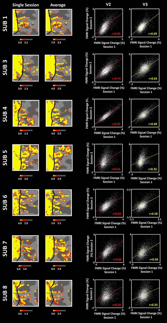
Consistency of the activity maps across scan sessions in one subject (Subject 2). A–C, Maps of color-selective activity (as in Fig. 3), acquired independently in two sessions (A, B), plus the average of those two sessions (C). All maps show strong similarities among the activity recorded during the first, second, and averaged activity. The averaged map is statistically stronger than either of the two component images, as reflected in the higher thresholds in the right panel (see activity scale bars). Scale bar, 5 mm. D, E, The correlation of BOLD values (color vs luminance) between the two sessions (p > 10−3). Each white dot represents activity in one vertex within either the left or right hemisphere, in the first vs second scan sessions, throughout the activated representation of V2 (D) and V3 (E).

Consistency across sessions in all seven remaining subjects. Each row shows data from one subject. Maps from a given cortical location are shown for one individual and group averaged scan sessions (first and second columns, respectively). The third and fourth columns show between-session correlation plots in V2 and V3, respectively. In all subjects, the level of correlation between activities recorded in the two independent sessions was highly significant (p > 10−3). Other details are as in Figure 4.
In V2, patchy stripes were generally consistent with the predicted topography of thin stripes in humans. First, the long axis of the stripes was aligned approximately perpendicular to the V1–V2 border. Second, the spacing between adjacent color-selective stripes averaged 7.22 ± 0.77 mm (center-to-center, measured along the folded cortical surface mesh, sampled in all 16 hemispheres). As predicted (Tootell and Taylor, 1995), this spacing was approximately twice that found in NHPs. Third, such stripes were not found in V1, at representations peripheral to the retinotopic limit of stimulus-driven activity (Fig. 3B). Instead, V1 showed a generally higher response to color, presumably reflecting strong and spatially undifferentiated activity in 4Cb (Tootell et al., 1988b), plus lower color-biased activity to this stimulus in layers 2 and 3.
Color-selective columns in V3
Comparison of the above maps to the retinotopic maps revealed additional color-selective sites, some located within the stimulus-activated retinotopic representation in V3 (Fig. 3B). Often, these V3 sites took the form of isolated columns, rather than elongated stripes. Some V2 stripes appeared to extend confluently into V3 color-selective columns or stripes. However, such across-border confluence may be coincidental.
Consistency across sessions
Our experiments combined data from two independent scan sessions. To validate this approach, we compared the two single-session maps to the combined map in each subject, testing for the following: (1) an expected increase in CNR in the combined maps; and (2) consistency (reliability) across the two sessions. Figure 4 illustrates this comparison in one hemisphere. The two single-session fMRI maps were quite similar to each other (Fig. 4A,B). Moreover, the combined map supported a higher CNR compared with either of the single-session maps, as reflected in the higher significance values in Figure 4C.
To measure this relationship more systematically, we measured the correlation between the percentage signal change of the BOLD signal to the color-versus-luminance stimulus contrast, across the two scan sessions, at each cortical surface mesh vertex, measured independently in V2 and V3 (Fig. 4D,E). In each area, the correlation coefficient was quite high in both V2 (r = 0.73) and V3 (r = 0.62), and well above the level of chance (p < 10−3; see Materials and Methods). Figure 5 shows analogous data from all remaining (n = 7) subjects. In all eight subjects, the correlation coefficient exceeded r > 0.33 (p < 10−3). These results confirm high consistency in our activity maps.
Variation with cortical depth/layers
To the extent that our fMRI results reflect classic cortical columns, our maps should be similar to each other across different cortical depths/layers. An analogous consistency of maps across depths/layers was demonstrated using deoxyglucose labeling of ocular dominance columns (ODCs) in V1 (Tootell et al., 1988a).
However, a second factor complicates this prediction here: it is known that large draining pial veins also contribute to measured BOLD responses (Polimeni et al., 2010). Presumably, such a pial contribution would blur and displace measured responses away from the neuronal activity, thus causing errors in the BOLD maps measured near the pial surface. However, additional data suggest that the pial vein contribution is significantly lower (if not zero) in the deeper cortical depths (e.g., layers 5 and 6; Polimeni et al., 2010), where our BOLD responses were measured (see Materials and Methods).
Both of these influences were evident in our data (Fig. 6). Maps from the deep cortical depths showed quite regular and periodic spatial patterns, which is consistent with the topography predicted for color-selective thin stripes in human V2. Maps centered in the middle depths were quite similar to those maps in deeper cortex, which is consistent with a radial (columnar) component across lower and middle layers. Given the size of the voxels used here (1.0 mm, isotropic) and the average cortical thickness (see Materials and Methods), this similarity also likely reflects a contribution of common voxels spanning the deep and middle cortical layers.

Effect of depth variation in color-selective stripes/columns in V2/V3 of Subject 3. A–C, Color-selective activity in the superficial, middle, and deep cortical layers (see Materials and Methods), respectively. Generally, maps from the lower layers are similar to those in the middle layers, which is consistent with radially extending fMRI activity. However, maps from superficial layers (A) include large blotches, presumably arising from draining veins. Despite these large blotches, a few stripes/columns can be seen in these superficial maps, which correspond topographically to those in the middle and lower depths/layers (cyan arrowhead). Other details are as in Figure 3. The four graphs in D and E show the correlation of color-selective activity sampled across deep vs superficial layers of V2 and V3. The bottom two graphs show the analogous analysis along an orthogonal axis, sampled within a common (deep) depth/layer. Sampling length was equivalent in the across-column vs within-column analyses. The correlation was significantly higher between activities sampled within columns compared with across columns in V2 (z = 24.98) and V3 (z = 28.88) areas, suggesting a strong columnar component in our BOLD maps.
In contrast, maps from superficial depths (including layers 1 and 2) were dominated by larger scale blotches, consistent with an artifactual spatial blurring (and/or displacement) caused by the pial vasculature (Fig. 6A–C). Despite this presumptive pial contribution, a few apparent color-selective stripes also exceeded the statistical threshold in the more superficial layers, which matched the location of color-selective stripes in deeper layers—apparently reflecting nearby BOLD responses within a cortical column near the cortical surface. Importantly, only a negligible number of voxels could contribute to the deep and superficial (pial) cortical activity maps.
Thus, despite the potential confound of pial vessel contamination in the upper layers, a columnar component might still be evident in a more quantitative analysis of BOLD activity evoked by the color-versus-luminance stimuli. To test this possibility, we compared the correlation between the measured percentage of signal change of the BOLD responses at the two depth extremes (e.g., in our upper vs lower layers). In all subjects, this correlation was significant, supporting a radial (columnar) component. In a control analysis, we also measured the correlation between nearby vertices in the tangential direction (with a distance equivalent to the cortical thickness at those locations) within the deep layers (see Materials and Methods). This comparison confirmed a significantly higher correlation between vertices along the radial direction, compared with the correlation between vertices along the tangential direction, in all subjects (Figs. 6D,E, 7). Similar results were found in data from single sessions (data not shown here).

Analogous analyses of columnar organization (as described in Fig. 6) from the remaining seven subjects. Again, the data show a stronger correlation between activities sampled within columns compared with across columns in V2 (z > 9.17) and V3 (z > 8.32). This supports a columnar organization in all subjects.
Thus, overall, our evidence suggests that V2/V3 color-selective BOLD activity is columnar in three dimensions, despite an additional influence due to the layout of the large-diameter vessels overlying the cortical surface (see Discussion).
Disparity-selective stripes/columns
Next, we tested for stripes or columns that responded selectively to disparity-based stimuli in V2 and V3 (n = 6; see Materials and Methods). All subjects confirmed that the stereoscopic cuboids were robust and clearly distinguishable from the control stimulus.
This stimulus contrast produced stripes of higher disparity-selective activity, which is consistent with the predicted topography of thick stripes in human V2 (Fig. 8A). Disparity-selective columns were also found in V3. Consistent with previous fMRI studies in humans (Tsao et al., 2003; Bridge and Parker, 2007; Minini et al., 2010), activity was slightly higher throughout V1 in the disparity condition. However, no consistent topographical variations were found in V1 based on disparity.

Activity maps produced by two types of ocular interaction. A, Disparity-selective activity in Subject 1, to facilitate comparisons with Figure 3B. The disparity-varying stimulus produced clear stripes/columns within areas V2 and V3, compared with zero disparity stimuli. B, Well known pattern of ocular dominance columns evoked by binocular vs monocular stimuli in the same subject. This map showed systematically spaced stripes largely confined to area V1. Scale bar, 1 cm.
In V2, additional properties in the disparity-selective stripes were similar to those found for the color-selective stripes. For instance, the spacing between adjacent disparity-selective stripes averaged 7.22 ± 0.85 mm (center to center along the folded cortical surface; sampled in all 12 hemispheres). Similarly, intersession reliability was high for the disparity maps (Fig. 9).

Consistency across sessions for the disparity-selective stimulus contrast, for all six subjects tested, in areas V2 (left) and V3 (right). Here again, all subjects showed a correlation between activities recorded in the two independent sessions that was highly significant (p > 10−3). Other details are as in Figure 5.
Ocular dominance
As control conditions, we also presented RDSs monocularly to either left or right eyes, independently in different blocks, in four of the six main subjects. As expected, subtractive comparisons of these two conditions produced a pattern of ODCs throughout the stimulus-activated representation of the visual field (Fig. 8B). Beyond V1, additional regions of monocular bias were not consistently observed.
To measure the distance between ODC columns more precisely, for one subject (Subject 1), we mapped ODCs using higher-resolution scans based on voxels of 0.8 × 0.8 × 0.8 mm (see Materials and Methods), averaged across three different scan sessions. Figure 10 shows the map of ODCs in this subject based on voxels of 0.8 × 0.8 × 0.8 mm (Fig. 10A,B), voxels of 1.0 × 1.0 × 1.0 mm (Fig. 10C), along with ODCs measured in two other subjects based on voxels of 1.0 × 1.0 × 1.0 mm (Fig. 10D,E). According to this measurement (in Subject 1), ODCs are located ∼2.49 ± 0.63 mm (center to center of common eye input) from each other. This distance is similar to that reported previously in human ODCs based on fMRI (Cheng et al., 2001; Yacoub et al., 2007).

A, Map of ODCs within one hemifield of Subject 1 based on a voxel size of 0.8 mm, isotropic. B, C, Enlarged ODCs within a V1 subfield (A, yellow square) acquired using voxels of 0.8 and 1.0 mm (isotropic) during independent scan sessions. The overall pattern of ODCs remained similar across the two spatial resolutions. D, E, ODCs in two other subjects (3 and 6) acquired using voxels of 1.0 mm isotropic, as in C.
The true spatial sampling is expected to be somewhat larger in the phase-encoding direction due to T2 * blurring and partial Fourier effects (see Materials and Methods). However, because of the folded nature of the cortex relative to the phase-encoding direction, plus the irregular pattern of ODC stripes within V1 demonstrated with anatomical imaging, we do not expect that this blur contributed any substantial bias in the measurements of ODC stripe width.
We also quantitatively measured the consistency between activity maps acquired across different scan sessions, as has been done above for color-selective (Fig. 5) and disparity-selective (Fig. 9) stripes. In all four subjects for which ODC maps were available, we found a significant (p < 10−4) correlation between activity measured in V1 vertices across the two scan sessions (Fig. 11).

The consistency between ODC maps acquired in different scan sessions based on 1.0 mm (isotropic) voxels. Each panel shows the correlation between BOLD values (left vs right eye stimulation) between the two sessions (p > 10−3).
Obligate binocularity
Some studies in anesthetized NHPs have reported more generalized response increases to binocular stimuli in V2 thick stripes, regardless of the specific disparity (Roe and Ts'o, 1995; Chen et al., 2008). Such general responses have been termed “obligate binocular.”
Accordingly, we tested for obligate binocularity based on fMRI in awake humans. Using the data described above (n = 4), we compared responses to RDSs presented either (1) binocularly or (2) monocularly. Stimuli were otherwise equated (i.e., both lacked local disparity variations; the stereoscopic cuboids). In contrast to the results in Figure 8A, the binocular versus monocular stimulus comparison tested here did not produce selectively higher activity within the stereoscopically activated stripes/columns in V2 or V3. That is, we found no obligate binocularity in behaving humans.
Interdigitation of color and disparity stripes
In NHPs, the V2 thin stripes are centered midway between the thick stripes. Thus, these two CO dark stripe types are effectively interdigitated with each other, across intervening pale stripes. Here, we tested for an analogous interdigitation of color-selective versus disparity-selective stripes in human V2.
Simple activity overlays showed a strong tendency for interdigitation of color-selective versus disparity-selective patterns (Fig. 12), which is consistent with the thin stripe versus thick stripe model in V2 of NHPs. Analogously in V3, these overlays also suggested that color versus disparity columns are mutually segregated.

Evidence for an interdigitation of color-selective vs disparity-selective stripes/columns in V2/V3. Each row shows data from different subjects (Subjects 1, 2, and 5, from top to bottom). The leftmost panels show the color-selective maps. The middle panels show the disparity-selective maps, from the corresponding cortical locations. The disparity stripes/columns are outlined in black. The right panels show the overlay of color stripes (yellow-red activity map) and the disparity stripes/columns (black outlines). A strong tendency for nonoverlap is evident. The borders between V1, V2, and V3 are color coded as in the top left panel.
It could be argued that this evidence was complicated by the choice of threshold levels. All things being equal, higher activity thresholds should produce less overlap, compared with lower-activity thresholds. To address this concern, we first measured the extent of overlap between color-selective and stereo-selective stripes across a wide range of thresholds (−log(p) = 2–10). More specifically, at each threshold level, we measured the number of vertices that showed a color-selective and disparity-selective response, relative to the total number of vertices that showed either a color-selective or disparity-selective response. These measurements were conducted separately for V2 and V3. As a control, we also measured the extent of overlap when the organization of vertices in one map was randomly misaligned (i.e., spatially shuffled). Measurements were made from all six subjects in whom both color and disparity stripes were localized.
At all thresholds, the results showed more overlap when the patterns were misaligned compared with aligned, in both V2 and V3 (Fig. 13). In both areas, the application of a two-factor repeated-measures ANOVA (“threshold level” and “alignment”) yielded a significant effect of threshold level (F(16,80) > 20.53, p < 10−3), alignment (F(1,5) > 52.24, p < 10−3) and also a significant interaction between the two effects (F(16,80) > 5.52, p < 10−3). Thus, both the color and disparity stripes were systematically the least overlapped (e.g., interdigitated) in their native alignment (i.e., before spatial shuffling).

Overlap in the color-selective or disparity-selective maps, with variations in threshold and alignment, within V2 (left) and V3 (right). In both panels, the percentage of overlap (i.e., the number of vertices that show selectivity for color and disparity relative to the overall number of selective vertices) is shown for multiple threshold levels (in half-logarithmic steps), when the two maps were either precisely aligned (yellow) or topographically shuffled (cyan). Data were combined from all six subjects who participated in both Experiments 1 and 2. In both V2 and V3, the amount of overlap was significantly lower when maps were aligned rather than shuffled. Error bars indicate 1 SEM.
It might be argued that these results were potentially due to a strong bias for either color or disparity selectivity in V2/V3. Thus, we tested whether the number of color-selective and disparity-selective vertices differed significantly from each other, in each of these areas. Separate applications of two-factor repeated-measures ANOVA (“threshold level” and “selectivity-type”) to the number of selective vertices in V2 and V3 indicated that, while the number of color-selective and disparity-selective vertices in these areas varied significantly with the threshold level (F(16,80) > 59.22, p < 10−3), these numbers were essentially equal (F(1,5) < 0.58, p > 0.48) and the interaction between the two factors remained insignificant (F(16,80) < 0.54, p > 0.91). Thus, the decreased overlap between color and disparity stripes in these areas did not simply reflect a strong bias for either color or disparity selectivity.
This interdigitation suggests that the level of color-selective activity in V2/V3 stripes/patches might be negatively correlated with the level of disparity-selective response in these regions. Figure 14 shows the level of correlation between color-selective and disparity-selective activity, within V2 and V3 stripes/patches, measured across different selectivity levels. Measurements were made in those V2 and V3 vertices that showed a significant selectivity for either color or disparity stronger than −log(p) > 4(up to 10); this approach for defining color-selective and disparity-selective vertices avoided sampling from regions that were either nonresponsive (e.g., pale stripes) or overlapped (arising from either technical or biological factors). Results of this analysis showed the following: (1) in V2/V3 stripes/patches, there is a negative correlation between the level of color-selective and disparity-selective activity levels; and (2) in both areas, this correlation was significantly stronger (i.e., more negative) in vertices that showed higher selectivity for either color or disparity (F(12,60) > 7.75, p < 10−6).

Level of correlation between color-selective and disparity-selective vertices within V2 (left) and V3 (right). In both areas, the level of correlation was significantly (p < 0.05) stronger (more negative) than the chance level (i.e., r = 0). Error bars indicate 1 SEM.
Stripe width in human V2
Based on the eponymous width differences in the CO-based stripe in NHPs (Fig. 1), we next asked whether the color-biased fMRI stripes found in human V2 were measurably thinner, relative to (thicker) activity stripes driven by disparity. Observations appeared to support that idea (Figs. 3B, 8A). However, width measurements in the fMRI-defined stripes may covary with the chosen threshold level.
Therefore, we conducted an additional analysis. The thickness of color-selective and disparity-selective stripes was defined as the distance relative to the center of the stripe at which the fMRI signals lost half of their selectivity. Measurements were made in rows of V2 vertices aligned parallel with the V1–V2 border, across a systematically varied range of distances from that border, in all 12 hemispheres. We found that this “half-selectivity” point for color-selective stripes was located 2.42 ± 0.60 mm (mean ± SD) from the center of these stripes. In contrast, the half-selectivity point for disparity-selective stripes was located significantly further (paired-sample t test, t(11) = 2.55, p = 0.03) from the center of disparity-selective stripes (3.21 ± 1.03 mm). These results suggest that the color-selective stripes are indeed thinner, relative to disparity-selective stripes.
Stripe length in human V2
In the axis perpendicular to the above measurements, a different topographical feature also distinguishes these two CO-based stripe types in NHPs. Specifically, thin stripes extend contiguously to the V1–V2 border, without a gap. In contrast, thick stripes terminate short of the V1–V2 border (Fig. 1; Tootell et al., 1983). Accordingly, we hypothesized that the color-selective stripes in our fMRI maps might extend to the V1–V2 border, and the disparity-selective stripes would terminate short of that border. Again, observations generally supported this conclusion (Fig. 3B, 8A).
To test further for such a gap, we first measured the distance from the V1–V2 border for all vertices in V2 that showed either a significant color-selective or disparity-selective response (p < 0.05). Then, we tested whether the frequency of color-selective and disparity-selective vertices varied with distance relative to the V1–V2 border. Because the width of V2 varied across subjects, “distance” values were normalized relative to the width of V2 (see Materials and Methods).
The results were consistent with our hypothesis, in both the single and group-averaged data (Fig. 15). Color-selective vertices were detected frequently near the V1/V2 border, without an obvious discontinuity near that border. In contrast, we found a significantly lower percentage of disparity-selective vertices near the V1/V2 border, compared with the center of V2.

Evidence consistent with a topographic gap between V1 and fMRI-defined thick (but not thin) stripes. The figure shows the percentage of color-selective (top) and disparity-selective (bottom) vertices, across the normalized width of V2, relative to the V1/V2 border. The left panels show these data in Subject 5. The right panels show the group-averaged data from all six subjects. In all panels, the selectivity percentage was measured at the same threshold level (p = 10−2) for color and disparity maps. Fewer disparity-selective vertices were found near the V1/V2 borders relative to the color-selective vertices. This finding is consistent with CO-defined differences in thick vs thin stripes, respectively (e.g., Fig. 1).
Prior histological observations (Fig. 1) also suggest a mirror-symmetric decrease in CO staining located between the thick stripes and the anterior border between V2 and V3. Consistent with this hypothesis, Figure 15 shows that the distribution of disparity-selective vertices decreased near the border of V2 with V3.
Application of a two-factor repeated-measures ANOVA [stripe type (color vs disparity) versus distance from the V1–V2 border (0 vs 0.1 vs … vs 1)] showed a significant interaction between the effects of stripe type and distance (F(19,95) = 6.92, p = 0.01), supporting the notion that the frequency distribution of color-selective and disparity-selective vertices differed significantly from each other. Since it could be argued that (at least) part of this effect is due to uncertainty in location of those vertices adjacent to V1–V2 and V2–V3 borders, we repeated our tests after the exclusion of vertices whose distance relative to V2 borders was <5% of the V2 width. Results of this test still showed a significant stripe type × distance interaction (F(18,75) = 4.25, p < 10−5), suggesting that the frequency distribution of color-selective and disparity-selective vertices differed from each other regardless of uncertainty in the definition of V2 borders. Alternative interpretations of these data are also possible (see Discussion).
Functional connections
In all of the above tests, the fMRI variations were stimulus driven. To the extent that these results reflect two distinct functional networks, correlations in activity might be manifested even without visual stimuli, in measurements of resting-state functional connections.
To test this possibility, we acquired additional fMRI data in independent scan sessions. BOLD fluctuations were measured during the resting state with eyes closed, without any explicit task (see Materials and Methods). As seeds, we used the color-selective or disparity-selective V2 stripes and V3 columns, localized in each subject in Experiments 1–2. Correlations were measured between BOLD fluctuations in seeded areas relative to (1) functionally alike and (2) functionally unlike stripes/columns, in the opposite hemisphere, independently in both V2 and V3.
As shown in Figure 16, we found a higher correlation between spontaneous fluctuations of functionally alike (rather than unlike) stripes or columns in V2 and V3. The application of a three-factor repeated-measures ANOVA [“seeded stripes/columns” (color vs disparity) and “sampled stripes/columns” (color vs disparity), and “visual area” (V2 vs V3)] showed a significant interaction between the effects of seeded stripes/columns and sampled stripe/columns (F(1,5) = 7.66, p = 0.03), without significant interaction between the effect of area and the other two factors (F(1,5) = 1.58, p = 0.26).

Level of functional connection, measured during the resting state, between functionally alike and unlike stripes/columns in V2/V3 (left/right panels, respectively). Each panel shows the level of correlation between activity within color-selective and disparity-selective stripes/columns in V2/V3 after seeding color-selective (red) and disparity-selective (yellow) stripes/columns in the opposite hemisphere. These results suggest a relatively stronger functional connection between functionally alike rather than unlike stripes/columns in V2/V3.
Discussion
Area V2
In V2, relatively high color-selective responses have been localized to CO thin stripes based on invasive techniques in anesthetized (Hubel and Livingstone, 1987; Tootell et al., 1988a; Levitt et al., 1994b; Xiao et al., 2003; Lu and Roe, 2008) and awake (Tootell et al., 2004) macaque monkeys. Disparity-selective responses have been reported in CO thick stripes in relatively fewer studies of anesthetized (Hubel and Livingstone, 1987; Roe and Ts'o, 1995; Chen et al., 2008) and awake (Peterhans and von der Heydt, 1993) macaques.
Here we demonstrated functionally similar V2 stripes in awake humans, during stabilized attention. To the extent that our fMRI-based stripes in human V2 match expectations from prior results in NHPs, this result also validates our fMRI procedures for mapping columnar systems in V3.
On the other hand, we also found that several aspects of the human V2 stripes (e.g., lack of obligate binocularity) differed from those reported earlier in macaques. To the extent that the macaque visual system is regarded as a model for that in humans, such differences are important to define.
V2 stripes topography
Especially in some NHP species, the two thin and thick stripes differ quite markedly from each other, in both length and width (Fig. 1). Thus, we hypothesized that our functionally defined color-selective or disparity-selective stripes in V2 would show similar topographic differences. In contrast, it has been reported that CO-based differences in stripe width are not easily distinguished from each other in either humans (Adams et al., 2007) or macaques (Hubel and Livingstone, 1987; Levitt et al., 1994a; Shipp and Zeki, 2002).
Despite the latter reports based on CO, our fMRI data confirmed that color-selective versus disparity-selective stripes are indeed thinner and thicker, respectively. Moreover, the disparity stripes may also be shorter than the color stripes (Fig. 15). Specifically, disparity stripe topography was consistent with the hypothesis of a distinctive gap relative to the V1–V2 border, whereas analogous data from the color stripes extended contiguously to the V1–V2 border. With less certainty, our data supported CO evidence for an analogous gap between thick stripes with the V2–V3 border; if confirmed, this suggests that the shorter thick stripes are centered within V2. It may be important that such complementary differences in thickness and length will serve to minimize (or equate) the surface area in these two stripe types. The data in Figure 15 could also be interpreted to indicate progressive “thinning” of stripe width nearer the V1–V2 border, rather than (or in addition to) a “gap.”
In any event, our experimental approach may have emphasized these distinguishing topographic features. In NHPs, the topography of the CO-defined V2 stripes (including both the gap and the width differences) are most prominent in the middle and lower cortical layers (Tootell et al., 1983; Tootell and Hamilton, 1989; i.e., the layers from which our fMRI data were sampled).
Columns within V2 stripes
Relative to CO-defined stripes in some NHP species, the fMRI-labeled human stripes were arguably irregular or “patchy.” If confirmed, such a finding could reflect a straightforward species difference between humans and some NHPs. This interpretation is consistent with some (Tootell and Taylor, 1995) of the histological observations in humans. On the other hand, extreme patchiness has been noted in some thin stripes in CO patterns from macaque (Tootell and Hamilton, 1989; Sincich and Horton, 2002). Also, it is possible that fMRI activity reveals more patchiness compared with CO-based measurements, because these two measurements reflect quite different biological processes. In any event, the functional distinctions between these two different stripe types appear to be robust and evolutionarily conserved across tested catarrhine primates.
Area V3
Intriguingly, we also found functionally similar color-selective or disparity-selective patches in the “next” tier of information processing, area V3. Previously, little was known about possible functional columnar organizations in V3, despite a few intriguing observations in macaque monkeys. For instance, small CO-labeled patches/stripes were observed in cortically unfolded tissue, located in or near V3 (Lyon and Kaas, 2001; Sincich et al., 2003; Tootell et al., 2004). At least one of those high-CO patches/stripes showed color selectivity based on deoxyglucose (Tootell et al., 2004). Electrophysiological evidence also suggested disparity-selective columns in V3 (Adams and Zeki, 2001).
Functional connections
One could imagine that parallel (segregated) neuroanatomical connections might exist to support the functional segregation of color-selective or disparity-selective stripes/columns in V2 and V3. Our analysis of functional connectivity supports this idea (Fig. 16). It is tempting to associate these functional connections in humans to the more definitive tracer-based segregations known in different V2 stripes in NHPs (Hubel and Livingstone, 1987; Felleman and Van Essen, 1991; Sincich and Horton, 2002). Specifically, the double dissociation in our functional connections (color to color, disparity to disparity, with less cross-correlation) is consistent with this possibility of segregated connections in human V2 and V3.
However, variations in correlation between BOLD fluctuations during the resting state reflect multiple factors, some unrelated to neuroanatomical connections per se (Honey et al., 2009; Adachi et al., 2012).
Mapping columns using BOLD
A specific component of the cortical vasculature may have enhanced the columnar component in our results. Moderately small (20–150 μm) “diving” vessels extend radially throughout cortex (Duvernoy et al., 1983). Such vessels are sufficiently radial that they have been used as fiducial landmarks to align adjacent tangential sections in histological material (Livingstone and Hubel, 1984). Given the influence of local intracortical vascular anatomy on high-resolution fMRI data, and the potential for a coupling of the BOLD signal across depths from diving vessels, these vessels may have contributed to the radial (columnar) component in our maps.
On the other hand, the presence of such radial vessels cannot fully explain the functionally interdigitated stripes and columns observed here. The radial vessels are far scarcer, compared with the dense plexus of nonradial vessels extending throughout the gray matter. Nevertheless, these diving vessels are packed densely enough so that many of them “irrigate” each V2/V3 stripe/column. That is, our fMRI-based “columns” do not simply reflect BOLD spread from a single radial vessel located at the center of each column, analogous to a model suggested (Zheng et al., 1991; Harel et al., 2010), then largely refuted (Keller et al., 2011), in the smaller V1 blob–interblob organization. Additional studies in V1 also suggest that the organization of cortical columns is independent from the organization of these radial veins (Adams et al., 2015).
Previous columnar mapping studies in human fMRI
Several high-field fMRI studies have tested for ODCs in human V1 (Menon et al., 1997; Cheng et al., 2001; Yacoub et al., 2008), partly because ODCs furnish a well understood biological benchmark for imaging. Given these prior studies of columns in V1, it is somewhat surprising how little is known about the columnar organization of human extrastriate cortex based on fMRI, with a couple of exceptions. One notable exception (Goncalves et al., 2015) used a sophisticated fMRI approach, including averaging across sessions and sampling from middle cortical layers, to show increased clustering of disparity responses in and/or near area V3A. Another study (Zimmermann et al., 2011) reported evidence for axis of motion “features” in or near area MT/V5. However, neither study attributed their fine-scale activity variations to columns per se.
Pale stripes in V2
We did not test the functional properties of CO-based pale stripes, partly because the functional properties of the pale stripes remain somewhat undefined in NHPs. In any event, pale stripes are not reported to respond differentially to color or disparity. Thus, possible responses in pale stripes did not complicate the current results.
Conclusion
Architecturally, the organization of columns has numerous practical advantages for cortical information processing. Common functional properties can be preserved across layers, and interconnected via short radial processes. Longer intercortical connections can be sorted in different layers along each column.
Therefore, it is unsurprising that columns comprise a fundamental building block in many cortical areas, especially in visual cortex of NHPs. Speculatively, many additional types of columns may exist in human cortex, perhaps including higher-tier cortex. Such hypothetical sets of columns could remain undiscovered so far, partly due to technical limitations including spatial resolution. More subtly, such hypothetical columns could remain undiscovered because the underlying functional dichotomy was not deliberately tapped in a given experiment. For instance, the earliest studies of monkey V1 responses using circularly shaped stimuli did not (and could not) reveal orientation sensitivity in single units or in orientation columns (Hubel, 1982).
Activity in columns reveals fundamental properties of underlying neural activity, in a way that is less evident in fMRI signals measured across larger areas/regions. For instance, in previous measurements based on conventional fMRI, areas V2 or V3 did not show appreciable selectivity for either color (Hadjikhani et al., 1998; Liu and Wandell, 2005; Wade et al., 2008) or disparity (Tsao et al., 2003; Neri et al., 2004). Such results contrast with the results here, which showed strong color and disparity selectivity at the column level. Future column-level insights may clarify underlying single-neuron properties, which are often impossible to measure in humans.
Footnotes
- Received September 18, 2015.
- Revision received December 7, 2015.
- Accepted December 21, 2015.
This study was supported by Massachusetts General Hospital Executive Committee on Research (ECOR) fund Grant 2015A051305 to S.N. and R.B.H.T. Crucial support was also provided by the Martinos Center for Biomedical Imaging and National Institutes of Health (Grant 5P41-EB-015896-17), and by the help and cooperation of all of our subjects. We thank Dr. Douglas Greve for help in data analysis, Dr. Boris Keil for technical support, and Cesar Echavarria for help in making stimuli.
The authors declare no competing financial interests.
This is an Open Access article distributed under the terms of the Creative Commons Attribution License Creative Commons Attribution 4.0 International, which permits unrestricted use, distribution and reproduction in any medium provided that the original work is properly attributed.
- Correspondence should be addressed to Shahin Nasr, Athinoula A. Martinos Center for Biomedical Imaging, Massachusetts General Hospital, Charlestown, MA 02129. shahin{at}nmr.mgh.harvard.edu
- Copyright © 2016 Nasr et al.
This article is freely available online through the J Neurosci Author Open Choice option.