

Abstract
In the 1960s, Evarts first recorded the activity of single neurons in motor cortex of behaving monkeys (Evarts, 1968). In the 50 years since, great effort has been devoted to understanding how single neuron activity relates to movement. Yet these single neurons exist within a vast network, the nature of which has been largely inaccessible. With advances in recording technologies, algorithms, and computational power, the ability to study these networks is increasing exponentially. Recent experimental results suggest that the dynamical properties of these networks are critical to movement planning and execution. Here we discuss this dynamical systems perspective and how it is reshaping our understanding of the motor cortices. Following an overview of key studies in motor cortex, we discuss techniques to uncover the “latent factors” underlying observed neural population activity. Finally, we discuss efforts to use these factors to improve the performance of brain–machine interfaces, promising to make these findings broadly relevant to neuroengineering as well as systems neuroscience.
- motor control
- motor cortex
- dynamical systems
- brain-machine interfaces
- neural population dynamics
- machine learning
Introduction
Our knowledge of the motor cortices (MC) is rapidly evolving. Traditional models of motor cortical activity held that the firing rates of individual neurons “represent” externally measurable movement covariates, such as hand or joint kinematics, forces, or muscle activity. Much effort in related studies was devoted to finding the “correct” coordinate system. However, the increased ability to record from many neurons simultaneously has revealed many features of population activity that are difficult to reconcile with a purely representational viewpoint. First, much of the observed, high-dimensional activity of neural populations in MC can be explained as a combination of a modest number of “latent factors”; abstract, time-varying patterns that cannot be observed directly, but represent the correlated activity of the neural population. Second, during movements, these factors appear to evolve in time by obeying consistent dynamic rules, much like the lawful dynamics that govern physical systems. Through this lens, the complex, often-puzzling responses of individual neurons are naturally explained as minor elements in a coordinated underlying dynamical system. These findings have provided a new framework for evaluating neural activity during many of the functions that are ascribed to MC, such as motor preparation and execution, motor learning, bimanual control, and the production of muscle activity.
Beyond its application to the motor cortices, the dynamical systems framework and related computational methods may have broad applicability throughout the brain. Over the past decade, the ability to record from large populations of neurons has increased exponentially (Stevenson and Kording, 2011; Sofroniew et al., 2016, Jun et al., 2017; Stringer et al., 2018). These data collection tools promise to further transform our understanding of the brain, but only if we can process and interpret the coming wave of massive datasets. Trying to interpret the “tuning” of 10,000 neurons is not only onerous but a missed opportunity; much of the brain's computation is inaccessible from the activity of individual neurons, but is instead instantiated via population-level dynamics. Fortunately, modeling neural populations as low-dimensional dynamical systems is providing new insights in many cortical areas, including areas that mediate cognitive processes such as decision-making (Mante et al., 2013; Raposo et al., 2014; Carnevale et al., 2015), interval timing (Remington et al., 2018), and navigation (Harvey et al., 2012; Morcos and Harvey, 2016). This has deep implications for systems neuroscience: moving forward, the central thrust in understanding how brain areas perform computations and mediate behaviors may be through uncovering their population structure and underlying dynamics. MC is a critical model for studying these phenomena, as its activity appears strongly governed by internal dynamics, yet is well related to observable behavior. These characteristics make MC an excellent “proving ground” for tools that may be useful in a wide variety of brain areas.
Furthermore, our increasing knowledge of latent factors and dynamics in MC creates new opportunities to harness cortical activity to build high-performance and robust brain–machine interfaces (BMIs) to restore mobility to people with paralysis. BMIs aim to restore function by directly interfacing with the brain and reading out neural activity related to a person's movement intent. To date, the vast majority of BMIs that use MC activity have been based on a representational viewpoint, with the assumption that individual neurons represent external movement covariates. Incorporating knowledge of the latent structure and dynamics of MC population activity potentially offers the means to develop BMIs whose performance and long-term stability are greatly improved.
Our review is divided to cover three broad areas: (1) an overview of the dynamical systems view of MC, including key studies that have tested its applicability and demonstrated new insight into the structure of population activity in MC; (2) current techniques to uncover latent structure and dynamics from the activity of neural populations; and (3) recent efforts to use latent factors and dynamics to improve BMI performance.
The dynamical systems view and evidence in motor cortex
Early work to understand the relationship between MC activity and movements drew inspiration from studies in sensory areas, such as the experiments of Hubel and Wiesel (1959) in visual cortex. In those experiments, the response of a neuron was modeled as a function of carefully controlled features of the presented stimuli (Hubel and Wiesel, 1959). Similarly, studies in MC revealed that the responses of individual neurons (e.g., spike counts over hundreds of milliseconds) could be reasonably well modeled as a function of kinetic or kinematic movement parameters (Evarts, 1968; Georgopoulos et al., 1982; Schwartz et al., 1988). A complication of the motor domain is that these movement covariates could only be studied by training animals to produce highly stereotypic movements, replete with many correlations across limb segments and measurement systems. Over the next decades, a long-simmering debate that had originated perhaps with Hughlings Jackson over which parameters of movement were represented (Jackson, 1873; Phillips, 1975) was given new fuel. Anatomical considerations argue for a strong, direct link between primary motor cortex and muscle activity (Landgren et al., 1962; Jankowska et al., 1975; Cheney and Fetz, 1985), supported by many studies which found that neural activity covaries with muscle activation and kinetics (Evarts, 1968; Hepp-Reymond et al., 1999; Gribble and Scott, 2002; Holdefer and Miller, 2002). Yet correlates of higher-level parameters such as endpoint position (Riehle and Requin, 1989), velocity (Georgopoulos et al., 1982), speed (Churchland et al., 2006a), and curvature (Hocherman and Wise, 1991) could all be found as well. As this list became longer, some began to notice that these representations could also break down quite badly (Fu et al., 1995; Churchland and Shenoy, 2007b), and that such correlations could be spurious (Mussa-Ivaldi, 1988). This led many to wonder whether viewing MC as a representational system is appropriate (Fetz, 1992; Scott, 2008; Churchland et al., 2010).
Rather than asking which parameters constitute the output of MC, one might instead view the system from a generative perspective: how does MC generate its output? From this perspective, MC is seen as a computational engine whose activity translates high-level movement intention into the complex patterns of muscle activity required to execute a movement (Todorov and Jordan, 2002; Scott, 2004; Shenoy et al., 2013). If so, how might this computation be performed?
For decades, theoreticians have posited that brain areas may perform computation through network-level phenomena in which information is distributed across the activity of many neurons, and processed via lawful dynamics that dictate how the activity of a neural population evolves over time (for review, see Yuste, 2015). We formalize this dynamical view in Fig. 1A. We assume that at a given time point t, the activity of a population of D neurons can be captured by a vector of spike counts n(t) = [n1(t), n2(t), … nD(t)]. The neural population acts as a coordinated unit, with a K-dimensional internal “state” x(t) = [x1(t), x2(t), … xK(t)]. In many brain areas, x(t) has been observed to be much lower-dimensional than the total number of observed neurons (i.e., K ≪ D; Fig. 1B; Cunningham and Yu, 2014). This dimensionality is likely somewhat constrained due to the recurrent connectivity of the network, which restricts the possible patterns of coactivation that may occur (for review, see Gallego et al., 2017a). A notable consideration, however, is that the observed dimensionality is often lower than might be expected due to network constraints alone; this particularly low dimensionality may be further induced by the simplicity of common behavioral paradigms (Gao and Ganguli, 2015; Gao et al., 2017).

Intuition for latent factors and dynamical systems. A, n(t) is a vector representing observed spiking activity. Each element of the vector captures the number of spikes a given neuron emits within a short time window around time t. n(t) can typically be captured by the neural state variable x(t), an abstract, lower-dimensional representation that captures the state of the network. Dynamics are the rules that govern how the state updates in time. For a completely autonomous dynamical system without noise, if the dynamics f(x) are known, then the upcoming states are completely predictable based on an initial state x(0). B, In a simple three-neuron example, the ensemble's activity at each point in time traces out a trajectory in a 3-D state space, where each axis represents the activity of a given neuron. Not all possible patterns of activity are observed, rather, activity is confined to a 2-D plane within the 3-D space. The axes of this plane represent the neural state dimensions. Adapted from Cunningham and Yu, 2014. C, Conceptual low-dimensional dynamical system: a 1-D pendulum. A pendulum released from point p1 or p2 traces out different positions and velocities over time, and the state of the system can be captured by two state variables (position and velocity). D, The evolution of the system over time follows a fixed set of dynamic rules, i.e., the pendulum's equations of motion. Knowing the pendulum's initial state [x(0), filled circles] and the dynamical rules that govern its evolution [f(x), gray vector flow-field] is sufficient to predict the system's state at all future time points.
The dynamical systems view posits an additional constraint: the evolution of the population's activity in time is largely determined by internal rules (dynamics). In the limit of an autonomous dynamical system (i.e., a system that operates independently of any external factors), and without noise, the system's evolution follows the equation ẋ = f(x); that is, its future state changes are completely dependent upon (and predicted by) the current state. A conceptual example of a low-dimensional system with simple rotational dynamics (a 1-D pendulum), and its related dynamical flow-field, is presented in Figure 1, C and D. We note that MC clearly cannot be autonomous. It must receive and process inputs, such as sensory information, to produce responsive behaviors. However, as discussed below, the model of an autonomous dynamical system is reasonable for MC activity during the execution of well prepared movements. During behaviors that are unprepared, or where unpredictable events necessitate corrections (such as responding to task perturbations), MC activity may be well modeled as an input-driven dynamical system, analogous to a pendulum started from particular initial conditions, and subject to external perturbations (Pandarinath et al., 2018).
The dynamical systems framework makes testable predictions about the nature of MC activity. First, it predicts that the initial conditions of the system, such as those observed during movement preparation, largely determine the subsequent evolution of activity. Second, the activity of neurons in MC should relate not only to the inputs and outputs of the system, but also to the computations being performed. Finally, distinct computations may be appropriated into different, non-overlapping neural dimensions. Here, we explore experimental evidence related to each of these predictions.
Early studies exploring the dynamical systems hypothesis in MC examined whether preparatory activity served as an “initial condition” for the subsequent dynamics. In tasks with delay periods, where a subject has knowledge of the movement condition before execution, neural activity in MC approaches distinct “preparatory states” for distinct movements (Tanji and Evarts, 1976). In a dynamical system, initial conditions determine subsequent activity patterns, so the same dynamical “rules” can give rise to different activity patterns and behaviors if the initial condition is different. Similarly, in MC, an altered preparatory state relates to altered movement execution. If neural preparatory activity is not in the right state at the time of the go cue, either due to natural fluctuations (Churchland et al., 2006b; Afshar et al., 2011; Michaels et al., 2015, 2018), subthreshold microstimulation during the delay period (Churchland and Shenoy, 2007a), or a change in the location of the target (Ames et al., 2014), the reaction time is delayed compared with well prepared trials. This suggests that, if motor preparation is incorrect, subjects do not move until their preparation has been corrected. Furthermore, motor adaptation to a visuomotor rotation (Vyas et al., 2018), visuomotor scaling (Stavisky et al., 2017a), or a curl field (Perich and Miller, 2017; Perich et al., 2017) has been shown to modify the motor preparatory state. These modifications correspond to altered execution trajectories, and the associated changes in preparation states and execution trajectories transfer from covert settings (BMI tasks without movement) to overt movements (normal reaching movements; Vyas et al., 2018).
Additional work has tested whether dynamical system models continue to predict observed neural activity during the transition from preparation to movement. A simple model in which preparatory activity seeds the initial condition for rotational dynamics during movement generation fits neural activity well in nonhuman primates (Fig. 2A; Churchland et al., 2012; Elsayed et al., 2016; Michaels et al., 2016; Pandarinath et al., 2018) and humans (Pandarinath et al., 2015, 2018). Furthermore, recurrent neural networks trained to generate muscle activity after receiving preparatory input display dynamics similar to those recorded in MC (Hennequin et al., 2014; Sussillo et al., 2015; Kaufman et al., 2016), suggesting that a dynamical system that uses preparatory activity as the initial condition for subsequent movement dynamics may be a natural strategy for generating muscle activity during reaching.

Overview of results supporting the dynamical systems view of motor cortex. A, The neural state achieved during the delay period (green-red dots) predicts the subsequent trajectory of movement activity (green-red lines). Each dot/line is a single reach condition, recorded from a 108-condition task (inset). Adapted from Churchland et al., 2012. B, In dynamical systems, places where neighboring points in state space have very different dynamics are indications of “tangling”. Such regions would be highly sensitive to noise; small perturbations yield very different trajectories. C, Conceptual example illustrating tangling. Imagine a system that needs to produce two sine waves, one of which has double the frequency and is phase-shifted 1/4 of a cycle relative to the other. If it contains these sine waves with no additional dimensions, activity would trace out a figure 8, with a point of “high tangling” in the center. By adding in a third dimension, the system can move from a high tangling to a “low tangling” configuration, using the third dimension to separate the tangled points. Adapted from Russo et al., 2018. D, Although EMG often displays highly-tangled points (x-axis), MC's neural activity maintains low tangling (y-axis). E, Illustration of muscle-potent/muscle-null concept. Imagine a muscle that is driven with a strength equal to the sum of the firing rates of two units. If the units change in such a way that one unit's firing rate decreases as the other increases, then the overall drive to the muscle will remain the same (muscle-null). If, on the other hand, the neurons increase or decrease together, then the drive to the muscle will change (muscle-potent). In this way, neural activity can change in the muscle-null space while avoiding causing a direct change in the command to the muscles. Adapted from Kaufman et al., 2014. F, Neural activity in MC occupies a different set of dimensions during motor preparation than during movement. Red, Neural activity across different reach conditions in “preparatory” dimensions; green, neural activity across different reach conditions in “movement” dimensions. Adapted from Elsayed et al., 2016.
Another important prediction of the dynamical systems model is that not all of the activity in MC must directly relate to task parameters or muscle activity, but may instead relate to internal processes that subserve the current computation. For example, the switch from movement preparation to movement generation is accompanied by a substantial change in dynamics (Kaufman et al., 2014; Elsayed et al., 2016). Recent work has posited that this change is accomplished by a large, condition-invariant translation in state-space, which triggers the activation of movement-generation dynamics. Indeed, this condition-invariant signal is not only present at the switch from preparation to generation, but is also the largest aspect of the motor cortical response (Kaufman et al., 2016). Furthermore, during movement generation itself, the dominant patterns of neural activity may also play a role in supporting neural dynamics, rather than directly encoding the output. One challenge for a dynamical system results when the flow-field is highly “tangled”: when there are points in the space in which very similar states lead to very different future behavior. If two nearby points lead to different paths, then small amounts of noise in the system can lead to dramatic differences in the evolution of the neural state (Fig. 2B). A robust dynamical system, therefore, must ensure that the tangling is low, potentially by adding in additional dimensions of activity whose job is to “pull apart” points of high tangling (Fig. 2C). In MC, although some components of neural activity resemble muscle-like signals during movement generation, the largest patterns of neural activity during movement generation appear to function to reduce tangling (Fig. 2D; Russo et al., 2018). Thus, within MC, evidence has been found that some signals primarily support and drive dynamics, rather than directly encoding input or output.
Finally, the dynamical systems framework predicts that to perform different computations, neural activity may use different dimensions (Mante et al., 2013). Although this need not be a property of every possible dynamical system, using different dimensions for different functions allows a system to better maintain independence between its different roles. It has long been observed that many neurons are active both during movement preparation and movement generation. How then does preparatory activity avoid causing movement? Traditional views held that preparatory activity lies below a movement-generation threshold (Tanji and Evarts, 1976; Erlhagen and Schöner, 2002) or is under the influence of a gate (Bullock and Grossberg, 1988; Cisek, 2006). However, subthreshold activation fails to explain why preferred directions are minimally correlated between preparation and movement (Churchland et al., 2010; Kaufman et al., 2010), and there is little evidence for gating within MC, as inhibitory neurons in MC are not preferentially activated during motor preparation (Kaufman et al., 2013). The dynamical systems model, by contrast, makes a different prediction: that unwanted movements can be avoided by avoiding specific neural dimensions. Some dimensions, termed “output-potent”, correspond to activation patterns that are output to the muscles, whereas others, termed “output-null”, do not (Fig. 2D; Kaufman et al., 2014). In MC, different dimensions are activated during movement preparation and generation (Fig. 2E; Elsayed et al., 2016). Furthermore, the dimensions that best correlate with muscle activity are preferentially active during movement generation, suggesting that output-potent dimensions are selectively avoided during preparation (Kaufman et al., 2014). Similarly, distinct dimensions may be explored during cortically-dependent movement versus non-cortically-dependent movement (Miri et al., 2017), and sensory feedback initially enters MC in different dimensions from those of the muscle-potent activity (Stavisky et al., 2017b).
This division of different functions into different neural dimensions is not limited to muscle-related activity. In BMIs, where output-potent dimensions can be specified explicitly, activity that is informative about experimentally induced perturbations is initially orthogonal to the corresponding corrective responses (Stavisky et al., 2017b). During long-term BMI use, activity in output-potent dimensions is more stable than output-null dimensions (Flint et al., 2016). Neural activity also tends to occupy different dimensions for different movement categories: for example, pedaling in a forward versus reverse direction (Russo et al., 2018), isometric force production versus limb movement (Gallego et al., 2017b), or moving with the contralateral versus ipsilateral arm (Ames and Churchland, 2018). Using different neural dimensions for different functions may give the MC flexibility to generate activity patterns that support a wide variety of functions without interfering with one another (Perich et al., 2017).
Methods for estimating and evaluating motor cortical dynamics
As detailed above, much of the activity of MC neurons is naturally explained as a reflection of a low-dimensional dynamical system. Studying such dynamic processes requires techniques that can infer latent structure and its dynamics from observed, high-dimensional data. Related techniques have been applied to a wide variety of model systems and brain areas over the last two decades (for review, see Cunningham and Yu, 2014). However, MC holds particular value for testing these techniques, as its activity is closely tied to observable behavior (e.g., movement conditions, arm or hand kinematics, reaction times), which provides a key reference for validating the inferred state estimates. In this section, we review common techniques for estimating latent state and dynamics that have been applied in MC. We first present a general framework for discussion. Next, we review techniques that are applied to time points independently (i.e., do not explicitly model neural dynamics). Finally, we review techniques that do explicitly model neural dynamics, thereby resulting in better latent state estimates.
Techniques for latent state estimation typically view spiking activity as being “generated” by an underlying state x(t) (Fig. 3A). A common assumption is that for any given trial, the observed high-dimensional spike counts n(t) reflect a noisy sample from each neuron's underlying firing rate distribution r(t), a distribution that is itself derived from the latent state x(t). For motor cortical data, the distinction between observations n(t) and underlying rates r(t) captures the empirical observation that the spiking of any given neuron across multiple repeats (trials) of the same movement is highly variable.

Applications of latent state and dynamics estimation methods to MC ensemble activity. A, Generative model of observed neural activity. Population spiking activity is assumed to reflect an underlying latent state x(t) whose temporal evolution follows consistent rules (dynamics). Firing rates for each neuron r(t) are derived from x(t), and observed spikes n(t) reflect a noisy sample from r(t). B, dPCA applied to trial-averaged MC activity during a delayed reaching task separates condition-invariant and condition-variant dimensions. Each bar shows the total variance captured by each dimension, with red portions denoting condition-invariant fraction, and blue portions denoting condition-variant fraction. Traces show projection onto first dimension found by dPCA. Each trace corresponds to a single condition (inset, kinematic trajectories with corresponding colors). Adapted from Kaufman et al., 2016. C, GPFA reveals single-trial state space trajectories during a delayed reaching task. Gray traces represent individual trials. Ellipses indicate across-trial variability of the neural state at reach target onset (red shading), go cue (green shading), and movement onset (blue shading). Adapted from Yu et al., 2009. D, SLDS enables segmentation of individual trials by their dynamics. Each horizontal trace represents a single trial for the first state dimension found by the SLDS. Trace coloring represents time periods with distinct (discrete) dynamics for each trial, recognized in an unsupervised fashion. Switching between dynamic states reliably follow target onset and precede movement onset, with time lags that are correlated with reaction time. Adapted from Petreska et al., 2011.
A standard approach to de-noising n(t) and approximating r(t) is trial-averaging. Trial-averaging assumes all trials of a given movement condition are identical, and reduces single-trial noise in the estimate of r(t) by averaging n(t) across repeated trials. r(t) is often further de-noised by convolving it with a smoothing kernel. A common approach to estimate the lower dimensional x(t) is to perform principal component analysis (PCA). Performing PCA on r(t) rather than n(t) is preferred; if performed on n(t), PCA often results in poor latent factor estimation, because it simply maximizes the variance captured by the low-dimensional space, without separating variance that is shared among neurons from variance that is independent across neurons (for review, see Yu et al., 2009). When performed on r(t), PCA is typically accompanied by firing rate normalization, so that neurons with high rates (and thus higher variability) do not dominate the dimensionality reduction. Further, PCA can be extended by integrating some supervision into the dimensionality reduction step, e.g., by integrating information about task conditions to identify dimensions that capture neural variability related to particular task variables, using de-mixed PCA (dPCA; Fig. 3B; Kobak et al., 2014; Kaufman et al., 2016; Gallego et al., 2017b). The strategy of trial-averaging followed by PCA has led to several insights into latent structure and dynamics in MC (Churchland et al., 2012; Ames et al., 2014; Kaufman et al., 2014; Pandarinath et al., 2015; Elsayed et al., 2016; Kaufman et al., 2016; Gallego et al., 2017b; Russo et al., 2018).
However, circumventing the need to average over trials is critical for elucidating inherently single-trial phenomena, such as the trial-to-trial variability of real movements (and their corresponding error corrections), non-repeated behaviors such as natural movements, random target tasks, and tasks involving learning. Likewise, studying “internal” processes that vary substantially across trials and have limited behavioral correlates, such as decision-making, vacillation, and internal state estimates (Golub et al., 2015; Kaufman et al., 2015), is also impossible with trial-averaged data. Factor analysis (FA; Everitt, 1984) is often favored for analyzing single-trial phenomena (Santhanam et al., 2009; Sadtler et al., 2014; Golub et al., 2015, 2018; Athalye et al., 2017). A key assumption of FA is that activity that is correlated across neurons represents “signal” [comprising the latent factors x(t)], and activity that is not correlated across neurons represents “noise”. This assumption matches the graphical model in Figure 3A. A recent, complementary approach to capturing trial-dependent variability in n(t) without corrupting the latent factors is to integrate information regarding trial ordering into the dimensionality reduction step, and introduce a set of “trial factors” that accommodate variability across trials, as in tensor components analysis (TCA; Williams et al., 2018).
A key limitation of the above techniques (PCA, FA) is that they treat neighboring time points as though they are independent. However, as discussed, a core assumption of the dynamical systems framework is that time points are intimately related, and in particular, previous states are predictive of future states. Therefore, methods that simultaneously infer latent states and dynamics should provide more accurate state estimation by leveraging the interdependencies of data points that are close in time. Two well developed families of models are Gaussian process-based approaches (Fig. 3C; Yu et al., 2009; Lakshmanan et al., 2015; Zhao and Park, 2017; Duncker and Sahani, 2018) and linear dynamical systems (LDS)-based approaches (Macke et al., 2011; Buesing et al., 2012; Gao et al., 2015, 2016; Kao et al., 2015, 2017; Aghagolzadeh and Truccolo, 2016). Gaussian Process approaches assume that the latent state x(t) is composed of factors that vary smoothly and independently in time, with each factor having its own characteristic time constant. In comparison, LDS-based approaches assume that the latent state at a given time point is a linear function of the previous state (i.e., ẋ = Ax), which incorporates linear interactions between latent dimensions. One issue with the LDS approach is that the matrix A is time-invariant, yet must capture the dynamics at all time points. In MC, this is potentially problematic, because activity during different behavioral phases (e.g., preparation and movement) is governed by very different dynamics (Kaufman et al., 2014, 2016; Elsayed et al., 2016). A promising approach to address this challenge is switching LDS (SLDS), which assumes that at any given time point, the system's evolution obeys one of a discrete set of possible dynamics, each of which must be learned (Fig. 3D; Petreska et al., 2011; Linderman et al., 2017; Wei et al., 2018).
An alternative approach to uncovering single-trial population dynamics uses recurrent neural networks (RNNs). Known as latent factor analysis via dynamical systems (LFADS; Sussillo et al., 2016a; Pandarinath et al., 2018), the approach trains an RNN as a generative model of the observed spiking activity. RNNs are powerful nonlinear function approximators, capable of modeling complex, highly nonlinear dynamics through adjustment of their recurrent connectivity (Fig. 4A). LFADS uses a sequential autoencoder (SAE) framework (Fig. 4B), allowing the potentially nonlinear dynamics to be learned from noisy, single-trial neural population activity using stochastic gradient descent. This allows LFADS to accurately infer dynamics on a single-trial, moment-to-moment basis (Fig. 4C). A critical confirmation that these dynamics are accurate and meaningful is that they lead to dramatic improvements in the ability to predict behavior. As shown (Fig. 4D), the LFADS-inferred latent representations were considerably more informative about subjects' reaching movements than was the population activity that was directly observed. These findings reinforce that population states, rather than the activity of individual neurons, may be a key factor in understanding how brain areas mediate behaviors, and further, that SAEs provide a powerful new avenue toward linking the activity of neural populations to the behaviors they mediate.
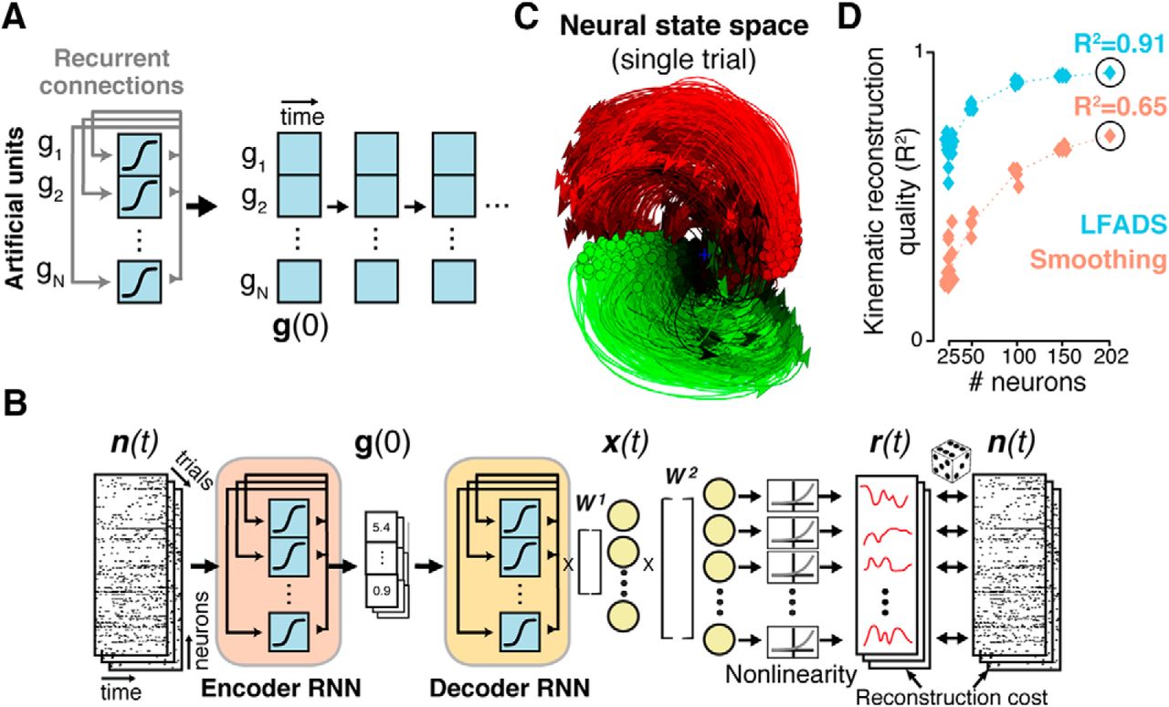
LFADS uses recurrent neural networks to infer precise estimates of single-trial population dynamics. A, A recurrent neural network (simplified) is a set of artificial neurons that implements a nonlinear dynamical system, with dynamics set by adjusting the weights of its recurrent connections. Conceptually, the RNN can be “unrolled” in time, where future states of the RNN are completely predicted based in an initial state g(0) and its learned recurrent connectivity (compare Fig. 3A). B, The SAE framework consists of an encoding network and decoding network. The encoder (RNN) compresses single-trial observed activity n(t) into a trial code g(0), which sets the initial state of the decoder RNN. The decoder attempts to re-create n(t) based only on g(0). To do so, the decoder must model the ensemble's dynamics using its recurrent connectivity. The output of the decoder is x(t), the latent factors, and r(t), the de-noised firing rates. C, The de-noised single-trial estimates produced by LFADS uncover known dynamic features (such as rotations; Fig. 2A) on single trials. D, Decoding the LFADS-de-noised rates using simple optimal linear estimation leads to vastly improved predictions of behavioral variables (hand velocities) over Gaussian smoothing, even with limited numbers of neurons. Adapted from Pandarinath et al., 2018.
Leveraging latent factors and dynamics for BMIs
BMIs aim to help compensate for lost motor function by directly decoding movement intent from neuron spiking activity to control external devices or restore movement (Taylor et al., 2002; Carmena et al., 2003; Hochberg et al., 2006, 2012; Ethier et al., 2012; Collinger et al., 2013; Sadtler et al., 2014; Gilja et al., 2015; Ajiboye et al., 2017; Pandarinath et al., 2017). BMIs have largely decoded neural activity into movement through a representational viewpoint: each neuron represents a reach direction and if the neuron fires, it votes for movement in that direction (Georgopoulos et al., 1982; Taylor et al., 2002; Gilja et al., 2012; Hochberg et al., 2012; Collinger et al., 2013). Efforts to decode EMG activity have been essentially similar, though in a higher-dimensional, more abstract space (Pohlmeyer et al., 2007; Ethier et al., 2012). However, as previously discussed, this representational model has important limitations in describing MC activity. In this section, we review recent studies that have asked whether representational assumptions also limit BMI performance, and if so, whether performance and robustness can be increased by incorporating MC latent factors and dynamics.
Using latent factors and dynamics to increase BMI performance
The dynamical systems view holds that movement-related variables (such as kinematics or EMG activity) are not the only factors that influence the activity of MC neurons. However, BMI decoders based on the standard representational model do not take other factors into account when relating observed activity to movement intention. Recent work introduced a decoding architecture (graphically represented in Fig. 5A) that incorporates latent factors and their dynamics (modeled as a simple linear dynamical system; Kao et al., 2015; Aghagolzadeh and Truccolo, 2016). One advantage of this architecture is that modeling latent factors can account for the multiple, diverse influences on observed neural activity to better uncover movement-related variables. A second advantage is that latent factors may be more easily de-noised than the observed high-dimensional activity, resulting in higher BMI performance. Briefly, the dynamical systems view assumes that the temporal evolution of MC states is largely predictable. If so, deviations from this prediction may primarily correspond to noise. To de-noise, MC dynamics can be used to adjust the latent factors so that they are more consistent with the dynamic predictions (Fig. 5B). In closed-loop BMI experiments, decoding the dynamically de-noised latent factors significantly increased performance over previous approaches (Fig. 5C), including previous representational decoders that de-noise activity by (1) smoothing using an experimenter-chosen filter (optimal linear estimator; Velliste et al., 2008; Collinger et al., 2013), (2) incorporating prior knowledge about kinematic smoothness (kinematic Kalman filter; Wu et al., 2003; Kim et al., 2008; Gilja et al., 2012, 2015; Hochberg et al., 2012), and (3) learning filtering parameters via least-squares regression (Wiener filter; Carmena et al., 2003; Hochberg et al., 2006).

Improving BMI performance and longevity by leveraging neural dynamics. A, Graphical model of decoder with dynamical smoothing. B, Illustration of smoothing latent state estimates using neural dynamics. The instantaneous estimate of the latent state (blue) is augmented by a dynamical prior (gray flow-field) to produce a smoother, de-noised estimate (orange). C, Smoothing using neural dynamics results in better closed-loop BMI performance than other approaches. Performance is achieved information bitrate. Adapted from Kao et al., 2015. D, Example of low-dimensional signals that can be used to augment intracortical BMIs. PCA applied to neural activity around the time of target selection identifies a putative “error signal”, allowing real-time detection and correction of user errors in a typing BMI. Adapted from Even-Chen et al., 2017. E, Remembering dynamics from earlier recording conditions can extend performance as neurons are lost. Performance measure is (off-line) mean velocity correlation. F, Comparison of closed-loop performance when 110 channels are “lost” shows a >3× improvement achieved by remembering dynamics. FIT-KF, state-of-the-art kinematic Kalman filter (Fan et al., 2014). Adapted from Kao et al., 2017. G, Dynamic neural stitching with LFADS. A single model was trained on 44 recording sessions. Each session used a 24-channel recording probe. Left, Recording locations in MC. Right, Single-trial reaches from an example session. Arc. Sp., arcuate spur; PCd, precentral dimple; CS, central sulcus. H, Neural state space trajectories inferred by LFADS. Each trace of a given color is from a separate recording session (44 traces per condition). Inferred trajectories are consistent across 5 months. jPC1 and jPC2 are the first two components identified by jPCA (Churchland et al., 2012). I, Using LFADS to align 5 months of data (“Stitched”) significantly improves decoding versus other tested methods. Adapted from Pandarinath et al., 2018. ***Significant improvement in median R2; P < 10−8, Wilcoxon signed-rank test.
BMI performance may also be increased through the use of non-movement signals that become apparent by examining latent factors. Recently, Even-Chen et al. (2017) exploited this idea to identify factors that reflect errors made during BMI control. The motivation for this work is that errors inevitably happen when controlling a BMI; however, instead of the user having to correct an error explicitly, it is possible to detect (or predict) its occurrence and automatically correct it (or prevent it). They applied PCA to identify an error-related signal in MC and found dimensions where projected neural data reflected task errors (example latent factors observed during errors are shown in Fig. 5D). In real-time experiments with monkeys, these latent factors were decoded to both prevent and autocorrect errors, improving BMI performance.
Using dynamics and latent factors to increase BMI longevity
Ideally, a BMI's performance would be maintained indefinitely. However, neural recording conditions frequently change across days, and even within-day in pilot clinical trials, e.g., due to neuron death or electrode movement and failure (Barrese et al., 2013; Perge et al., 2013; Sussillo et al., 2016b; Downey et al., 2018), which can lead to decoding instability. Current approaches to solve this problem include decoding more stable neural signals (e.g., threshold crossings and local field potentials; Flint et al., 2013; Nuyujukian et al., 2014; Gilja et al., 2015; Stavisky et al., 2015), gradually updating decoder parameters using a weighted sliding average (Orsborn et al., 2012; Dangi et al., 2013), automated decoder recalibration by updating “tuning” estimates daily (Bishop et al., 2014), continuous recalibration by retrospectively inferring the user's intention among a set of fixed targets (Jarosiewicz et al., 2015), and training robust neural network decoders on a diversity of conditions using large data volumes (Sussillo et al., 2016b).
A separate class of approaches aims to exploit the underlying neural latent space, which, as a property of the neural population, should have a stable relationship with the user's intention that is independent of the specific neurons observed at any moment (Gao and Ganguli, 2015; Dyer et al., 2017; Gallego et al., 2017b; Kao et al., 2017; Pandarinath et al., 2018). However, it is challenging to relate the observed neurons from a given recording condition to the underlying latent space. Recent studies using supervised alignment strategies have demonstrated the potential of latent dynamics to maintain BMI performance. Kao et al. (2017) exploited historical information about population dynamics (Fig. 5E,F), finding that even under severe neuron loss, aligning the remaining neurons to previously learned dynamics could partially rescue closed-loop performance, effectively extending BMI lifetime. Alternatively, Pandarinath et al. (2018) trained a single LFADS model using data from 44 independently recorded neural populations spanning many millimeters of MC and 5 months of recording sessions (Fig. 5G,H). They then used a single linear decoder to map these latent dynamics onto kinematics (Fig. 5I). This work demonstrated that, in the absence of learning, a single, consistent dynamical model describes neural population activity across long time periods and large cortical areas, and yields improved off-line decoding performance for any given recording session than was otherwise possible.
Some settings lack data for supervised alignment, i.e., directly linking neural activity from new recording conditions to motor intent may be challenging (settings without structured behaviors, or where intent is less clear on a moment-by-moment basis). In these settings, unsupervised techniques may be useful for aligning data. Recently, Dyer et al. (2017) introduced a semi-supervised approach called distribution alignment decoding (DAD; Fig. 6A–C). This approach aims to map neural data from a new recording condition (new data) onto a previously recorded low-dimensional movement distribution. To do this, DAD first reduces the dimensionality of the neural data (using PCA or a nonlinear manifold learning technique), and then searches for an affine transformation to match the low-dimensional neural data to movements, by minimizing the Kullback–Leibler (KL)-divergence between the two datasets (Fig. 6B). Their results demonstrate that DAD can achieve similar performance to that of a supervised decoder that has access to corresponding measurements of neural state and movement, if the underlying data distribution contains asymmetries that facilitate alignment (Fig. 6C). Although a powerful approach for aligning neural and movement data, DAD solves a non-convex optimization problem with many local minima (Fig. 6B) by using a brute force search. To improve alignment and avoid having to first perform dimensionality reduction, neural network architectures such as generative adversarial networks (GANs; Goodfellow et al., 2014; Molano-Mazon et al., 2018) provide a potential method to learn nonlinear mappings from one distribution to another (Fig. 6D). By leveraging the fact that low-dimensional representations of neural activity are consistent across days and even subjects, distribution alignment methods like DAD or GANs provide a strategy for decoding movements without labeled training data from new recording conditions.

Distribution alignment methods for stabilizing movement decoders across days and subjects. A, Data dimensionality is first reduced, and then low-dimensional projections are aligned onto a previously recorded movement distribution. B, KL-divergence provides a robust metric for alignment (displayed as a function of the angle used to rotate the data). Many local minima exist (points 1, 2, 3, 4), which makes alignment difficult. C, Prediction accuracy of 2-D kinematics for distribution alignment decoding and supervised methods. Left, Accuracy of DAD using movements from Subject M (DAD-M), from Subject C (DAD-C), and using movements from both Subjects M and C (DAD-MC). Right, Standard L2-regularized supervised decoder (Sup) and a combined decoder (Sup-DAD), which averages the results of the supervised and DAD decoders. All results are compared with an Oracle decoder (far right), which provides an upper bound for the best linear decoding performance for this task. Adapted from Dyer et al., 2017. D, A schematic of a generative adversarial network strategy for distribution alignment across multiple days: generator network (left) receives new data and learns a transformation of the data to match the prior (from a previous day).
Conclusions
The increasing ability to monitor large numbers of neurons simultaneously will present new opportunities to study neural activity at the population level. Mounting evidence shows that this provides a qualitatively different window into the nervous system from that of single-neuron recordings, and that population-level dynamics likely underlie neural population activity across a wide range of systems. Here we reviewed recent evidence that such dynamics shape activity and drive behavior in MC, outlined key methods for inferring latent factors and dynamics that have been applied to MC activity, and showed how uncovering latent factors and dynamics can yield higher-performing and more robust BMIs. Continuing advances in recording technologies, algorithms, and computational power will enable studies of dynamics that were not previously possible, and further, may open new avenues for neural prostheses to address a wide variety of disorders of the nervous system.
Footnotes
This work was supported by a Burroughs Wellcome Fund Collaborative Research Travel Grant (C.P.) and NIH NINDS R01NS053603 (L.E.M.).We thank Steven Chase, Chandramouli Chandrasekaran, Juan Gallego, Matthew Kaufman, Daniel O'Shea, David Sussillo, Sergey Stavisky, Xulu Sun, Eric Trautmann, Jessica Verhein, Saurabh Vyas, Megan Wang, and Byron Yu for their feedback on the paper.
The authors declare no competing financial interests.
- Correspondence should be addressed to Chethan Pandarinath, Emory University, 101 Woodruff Circle Northeast, Atlanta, GA 30322-0001. chethan{at}gatech.edu


