Models of grid cell spatial firing published 2005–2011
- Department of Psychology, Center for Memory and Brain, Boston University, Boston, MA, USA
Since the discovery of grid cells in rat entorhinal cortex, many models of their hexagonally arrayed spatial firing fields have been suggested. We review the models and organize them according to the mechanisms they use to encode position, update the positional code, read it out in the spatial grid pattern, and learn any patterned synaptic connections needed. We mention biological implementations of the models, but focus on the models on Marr’s algorithmic level, where they are not things to individually prove or disprove, but rather are a valuable collection of metaphors of the grid cell system for guiding research that are all likely true to some degree, with each simply emphasizing different aspects of the system. For the convenience of interested researchers, MATLAB implementations of the discussed grid cell models are provided at ModelDB accession 144006 or http://people.bu.edu/zilli/gridmodels.html.
1. Introduction
The puzzling grid cell has become a popular topic in neuroscience due to its simultaneously simple behavioral firing correlate (the animal’s position) and complex spatial activity (a nearly regular hexagonal arrangement of spatial fields; Figure 1).
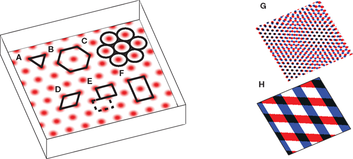
Figure 1. The grid cell spatial pattern. Different descriptions of the grid suggest different underlying mechanisms. The simplest descriptions as (A) an equilateral triangular tessellation or (B) a hexagonal grid suggest no obvious mechanism. (C) The pattern can be thought of as inactivity-surrounded place fields packed as closely as possible, which leads to Kropff and Treves (2008). Alternatively, the regularity of the pattern suggests that perhaps only a small segment, e.g., (D) a rhombus (skewed rectangle) or a rectangle large enough for (E) only one or (F) two or more appropriately spaced fields, is represented and when the animal walks off the segment it re-enters from the other side. If a rectangle containing only one field is used, it must be twisted so that walking off the bottom on the left brings the animal to the top on the right (the top edge is shifted by half its width, see dashed rectangle), while walking off the left or right sides wraps around normally. The grid can also be thought of as the overlap or interference between other spatial patterns, such as (G) smaller scale grids or (H) sinusoid-like gratings, not unlike a Fourier decomposition of the grid, and this produces the temporal interference models when generalized to the temporal domain. Note that in all figures spatial plots are shown in perspective to distinguish them from 2D plots of neural activities or synaptic weights.
From their spatial-coordinate–like appearance, persistence in darkness, head direction preference (in a subset of grid cells), and anatomical position in the medial temporal lobe (Hafting et al., 2005; Sargolini et al., 2006), all accounts of the hexagonal firing pattern assume grid cell firing is a function of the animal’s internal sense of its position. Most models specifically assume the grid cells are performing or reflecting path integration: the process of continuously updating an estimate of position with each movement made (McNaughton et al., 1996; Redish, 1999; Etienne and Jeffery, 2004). The current models of the hexagonal field arrangement therefore all start with path integration and then translate the path integrated information into the grid pattern through additional trickery (e.g., modifying the path integration mechanism to produce a hexagonal grid as a side effect or path integrating along directions in 60° or 120° increments and combining the separate integrated positions into a hexagonal pattern).
Existing grid cell models use a variety of different mechanisms, but similarities among models have led to a rough classification scheme (Burgess et al., 2007; Burgess, 2008; Giocomo and Hasselmo, 2008; Jeewajee et al., 2008; Kropff and Treves, 2008; Moser and Moser, 2008; Welinder et al., 2008; Burak and Fiete, 2009; Zilli et al., 2009; Milford et al., 2010; Zilli and Hasselmo, 2010; Giocomo et al., 2011; Yartsev et al., 2011; Mhatre et al., 2012) into the groups of continuous attractor network (CAN) models or of interference models, with some suggesting the true mechanism may involve both (Burgess, 2008; Hasselmo, 2008; Jeewajee et al., 2008). This terminology is somewhat misleading, though. For example, a number of models (Blair et al., 2007, 2008; Welday et al., 2011; Mhatre et al., 2012) use both CANs as well as the mechanism of interference (and see Discussion). The models can be better understood and compared when considered in terms of their subcomponents:
• How is the positional information encoded and maintained?
• How is the positional information updated when the animal moves?
• How is the encoded information read out as a hexagonal spatial pattern?
• How do any structured synaptic connections in the model self-organize?
As an example, Burgess et al. (2007) encoded positional information as the phase difference between oscillators, updated that position by modulating the oscillator frequencies, and used temporal interference to read that code out into the grid pattern. In these terms the space of models described in the literature becomes much clearer. For example, CANs are mechanisms for encoding and maintaining positional information, whereas interference is a read-out mechanism, so strictly the two are independent properties of a model.
Information-processing tasks (e.g., path integration) can be understood on multiple levels, three of which were emphasized by Marr (1982). On the highest level, tasks can be characterized by their goal (e.g., accumulate spatial displacements). A system can also be characterized by the way it represents the relevant data (e.g., phase differences, population activity patterns, etc.) and the algorithm that transforms the data (e.g., frequency modulation). Finally, a system has an implementation, mapping the representation and algorithm to physical systems. Tables 1 and 2 summarize the models with respect to the subcomponents above on the algorithmic and implementational levels, respectively. Though not all models fit perfectly into this system nor do all publications attempt to examine each of these aspects, this approach allows a useful overview of the field.
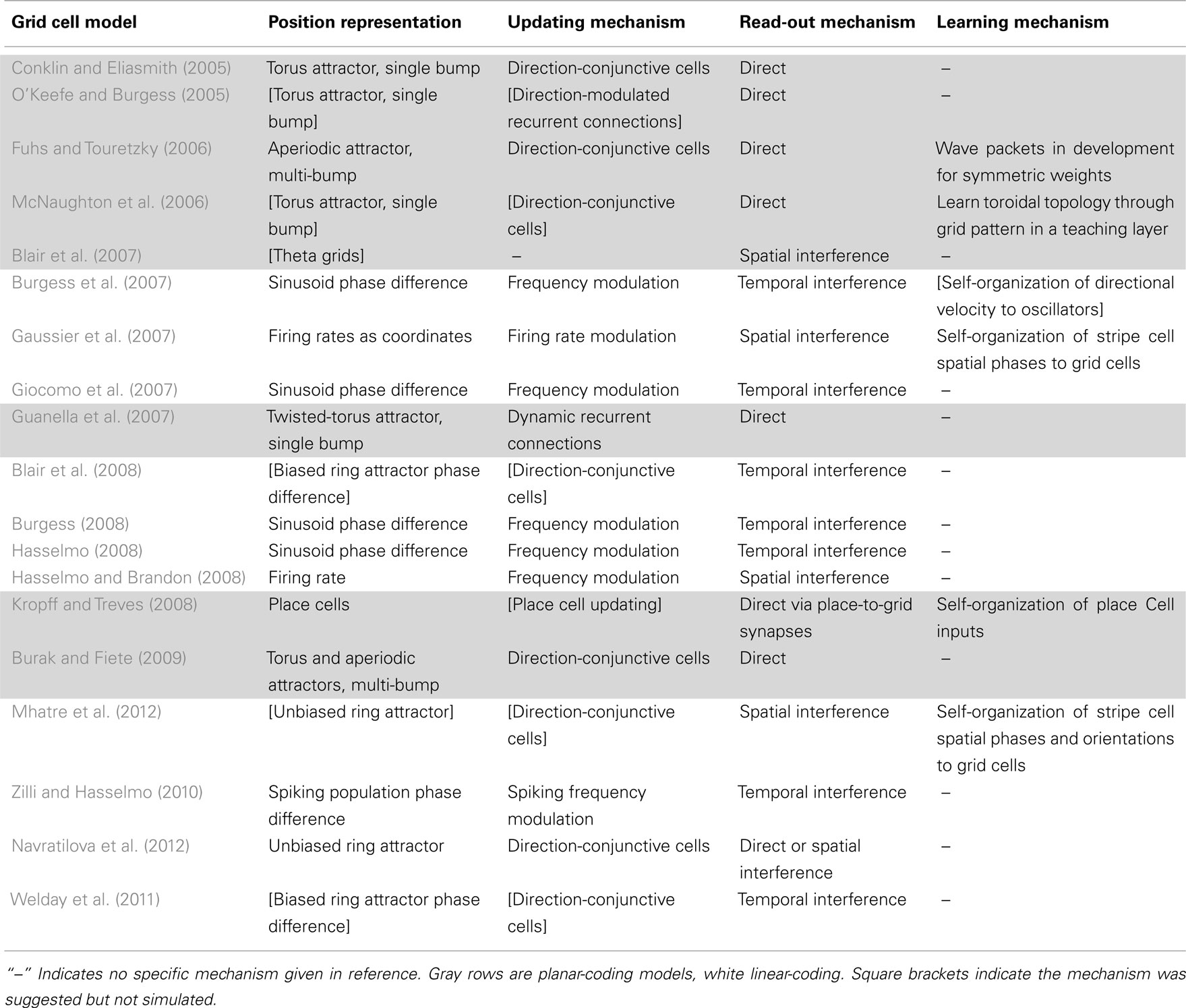
Table 1. The models on Marr’s algorithmic level.
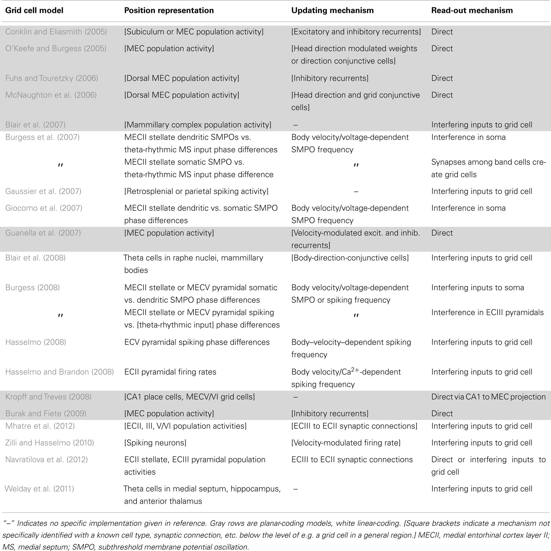
Table 2. The models’ biological implementations, though somewhat arbitrary, allow for concrete experimental predictions.
Below we discuss current approaches to the above questions before discussing each of the individual models. We hope our tight focus on model mechanisms complements other recent reviews (e.g., Welinder et al., 2008; Giocomo et al., 2011) that considered wider ranges of grid cell topics. For the convenience of interested researchers, we have also implemented in MATLAB most of the models of grid cells we are aware of and have shared them as a collection at ModelDB accession 144006 or http://people.bu.edu/zilli/gridmodels.html
2. Results
2.1. Encoding Positions
The starting point of all path integration models is a mechanism that allows neurons to represent and maintain a spatial position. These mechanisms can be divided into those that independently represent 1D positions and recombine them to form the 2D grid (linear-coding: Burgess et al., 2007; Gaussier et al., 2007; Giocomo et al., 2007; Blair et al., 2008; Burgess, 2008; Hasselmo, 2008; Hasselmo and Brandon, 2008; Zilli and Hasselmo, 2010; Welday et al., 2011; Mhatre et al., 2012) and those that directly represent 2D positions (planar-coding: Conklin and Eliasmith, 2005; O’Keefe and Burgess, 2005; Fuhs and Touretzky, 2006; McNaughton et al., 2006; Blair et al., 2007; Guanella et al., 2007; Kropff and Treves, 2008; Burak and Fiete, 2009; Navratilova et al., 2012). So far these suffice since grid cells seem to ignore height in simple 3D environments (Hayman et al., 2011).
2.1.1. Linear-coding
We first examine ways 1D positions can be encoded.
Perhaps the most obvious way of encoding a linear position is as a coordinate in a single cell’s firing rate. This mechanism was used by Gaussier et al. (2007) and Hasselmo and Brandon (2008), where respective scaling factors α or β Hz/cm translated distance moved along a cell’s preferred direction into a change in its firing rate. An advantage to directly storing distances from the starting position is that the return vector to the starting position can be easily calculated (e.g., Burgess et al., 1993; Touretzky et al., 1993; Hasselmo and Brandon, 2008), but since coordinates can be arbitrarily large (or negative) while cells can only fire over a limited frequency range, most models represent position less explicitly.
On linear tracks, grid cells have fairly regular field spacing (Brun et al., 2008). The fields seem to repeat endlessly so the animal’s 1D location can be encoded as a single number that gives its position relative to the nearest field (Figure 2A, top). Such a position is conveniently described in circular terms as a phase (an angle) in radians or degrees. A number of mechanisms for storing a phase have been used in grid cell models.
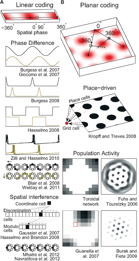
Figure 2. Spatial position codes. (A) Linear-coding models. Top. A linear track environment with three grid fields. Positions can be identified as a spatial phase between 0° in the center of one field and 360° (0°) at neighboring fields. One-quarter of the distance between the field centers, 90°, is indicated. Some models (Burgess et al., 2007; Giocomo et al., 2007; Blair et al., 2008; Burgess, 2008; Hasselmo, 2008; Zilli and Hasselmo, 2010; Welday et al., 2011) store the 90° linear position as a 90° phase difference between two oscillators. An unbiased (stationary) ring attractor (Mhatre et al., 2012; Navratilova et al., 2012) can also directly store the 90° phase as a bump of activity centered on cells in the ring at a corresponding angle. Instead of encoding position as a phase, the animal’s actual position or coordinate could be stored as the firing rate of a single cell (Gaussier et al., 2007). Hasselmo and Brandon (2008) described one model using only coordinate cells and another using only modulo cells. (B) Top. A square environment with many grid fields. Linear-coding models can encode 2D positions as two spatial phases, now measured between rows of grids, not neighboring grid fields (so only alternate 0° points are field centers). For example, a position at 0° along one direction and 90° along the other is indicated. Alternatively, place cells can represent 2D positions (Kropff and Treves, 2008) or a 2D position can be represented by the relative position of a fixed activity pattern on a sheet of cells (Fuhs and Touretzky, 2006; Guanella et al., 2007; Burak and Fiete, 2009). Early toroidal models, however, would produce a rectangular rather than a hexagonal grid. In continuous attractor network models each circle (Blair et al., 2008; Mhatre et al., 2012; Navratilova et al., 2012) or pixel (Fuhs and Touretzky, 2006; Guanella et al., 2007; Burak and Fiete, 2009) represents one cell and darker colors indicate higher activities. Red squares on the right indicate one cell that might produce the grid fields shown in the spatial environment.
A ring attractor is a CAN of neurons arranged in a circle, like the hours on an analog clock (illustrated in Figure 2A). In a simple ring attractor, any cell (e.g., 6 o’clock) strongly excites nearby cells (e.g., 4, 5, 7, and 8 o’clock) and weakly excites or even inhibits distant cells (e.g., 12 o’clock). When a small group of nearby cells is active (e.g., 6 and 7 o’clock) we call it a bump of activity. The cells mutually excite each other to continue firing while inhibiting the rest of the cells and so can store any phase value indefinitely by maintaining a bump of activity on the ring at that phase. We call this an unbiased ring attractor. Though our example used only one bump of activity, a larger network could easily support multiple bumps spaced out over the cells (see below and Figure 2B).
If the strongest output from each cell were systematically shifted in one direction, we could call it a biased ring attractor, cyclic attractor (Eliasmith, 2005), or ring oscillator (Blair et al., 2008). The bias causes the bump of activity to rotate around the ring at a fixed frequency that depends on the size of the network and the distance the peak output is shifted (Zhang, 1996). This asymmetry in the synaptic connections turns the network into an oscillator and so precludes storing a phase as a fixed bump of activity. Instead, a pair of biased ring attractors with identical frequencies can be used to store a phase in the difference between the phases of the rings (Blair et al., 2008). As the bumps move in the same direction and speed, the networks can maintain the phase difference indefinitely (Figure 2).
This mechanism of storing a phase with a pair of identical oscillators works with any oscillator imaginable (Figure 2A) as long as the oscillator can precisely and indefinitely maintain a specified frequency. Some early grid models (Burgess et al., 2007; Giocomo et al., 2007) interpreted the model oscillations as narrow-band oscillations in a cell’s membrane potential or in the local field potential (LFP; e.g., theta rhythm), though they were modeled abstractly as sinusoids. Other approaches manipulated the sinusoids to treat them as a rough approximation of repeating single spikes or burst of spikes (Burgess, 2008; Hasselmo, 2008). Unfortunately, data suggest biological oscillators like these are highly irregular (Welinder et al., 2008; Zilli et al., 2009; Dodson et al., 2011) and so unsuited for use in these models. One solution to this problem used synchronized networks of coupled, noisy, spiking neurons, which produce much more regular oscillations on the population level (Zilli and Hasselmo, 2010).
Using any of these mechanisms, a linear position can be represented neurally, but these mechanisms cannot represent a 2D position, which requires storing at least two values. Instead, to represent 2D positions, two or more independent linear-coding mechanisms can be used to encode linear position along two different directions (Figure 2B, top), requiring a read-out stage as described below.
An alternative is provided by planar-coding models.
2.1.2. Planar-coding
The planar-coding models represent the 2D position directly within one population of cells.
The simplest way of encoding a 2D position is through a Cartesian coordinate (x, y). A natural neural code for specific (x, y) positions is provided by the place cell: a cell that is nearly silent in all locations except in its place field, a small region of the environment where it fires at an elevated rate (O’Keefe, 1976; Skaggs et al., 1996). Place cells are used as the position code in Kropff and Treves (2008), the only non-path-integrating model of grid cells (though place cells could be driven by path integration).
Since grid cells themselves appear to code 2D positions, Blair et al. (2007) used high–spatial-frequency grid cells (Figure 1H) to encode and maintain 2D positional information. While they reported interesting results, using grid cells to produce grid cells somewhat lacks in explanatory power.
Just as 1D positions are identified with respect to the nearest two grid fields, 2D positions only need to be encoded in terms of position within, e.g., a rhombus whose corners are four adjacent fields (Figure 1D). So by analogy with an unbiased ring attractor in the linear-coding case, a 2D position can be encoded as a bump on a rectangular sheet of cells (Zhang, 1996; Samsonovich and McNaughton, 1997; Conklin and Eliasmith, 2005; O’Keefe and Burgess, 2005; McNaughton et al., 2006; Guanella et al., 2007; Figure 2B, right). Just as the ring attractor is essentially a string of cells with the ends connected to each other, the bump on the 2D sheet must be allowed to move off one edge of the sheet and reappear on the opposite edge.
A 2D sheet with opposite edges connected in this manner is called a torus. Such a network will generally produce rectangular, not hexagonal patterns. One solution (Guanella et al., 2007) that produces a hexagonal pattern is to twist the torus in such a way that the edges wrap around normally in one direction (e.g., left/right), but when a bump moves past, e.g., the top edge, it reappears on the bottom edge shifted by half the width of the torus (see Figures 1E and 2B, bottom). Strictly, though, this twist is not necessary and a normal torus can produce the hexagonal pattern if the velocity inputs are skewed (see below and our online model code for an example).
Rather than encoding position with a single bump of activity, a sheet of cells can maintain multiple bumps of activity, Figure 2B, arrayed hexagonally on the sheet of cells like each grid cell’s fields in space (Fuhs and Touretzky, 2006; Burak and Fiete, 2009). A cell’s adjacent fields occur not because a bump of activity wraps around one edge and returns to the cell, but rather because while the first bump moves off behind the cell, another bump comes from ahead. Bumps moving off one edge simply disappear while new bumps are created at the opposite edge. For this reason, a multi-bump CAN can produce the hexagonally arrayed fields without the need for synaptic connections wrapping around the edges. This is called an aperiodic network.
A multi-bump 2D CAN can also produce a hexagonal grid on an untwisted torus (a periodic network). In that case the bump spacing must be consistent with the size of the torus (Burak and Fiete, 2009).
2.2. Updating
With the above mechanisms a position can be represented and maintained, but the key to path integration is updating that representation of position as an animal moves from one place to another. In all models except (Kropff and Treves, 2008), changes in position are provided as a body velocity signal. Guanella et al. (2007) uses the 2D velocity signal directly, but the other models first pre-process 2D velocity into 1D directional velocity signals. The directional velocity vφ(t) along a preferred direction φ is defined as vφ(t) = s(t)cos(d(t) − φ), where s(t) and d(t) are the animal’s speed and direction at time t. Linear-coding models usually use two to six of these directional velocity inputs with preferred directions at increments of 60° or 120°, while planar-coding models generally assume four inputs at 90° increments (but would work with as few as three at 120° or up to a continuous distribution of all directions). Clear directional body velocity signals have not yet been found (but see Welday et al., 2011), but an analogous representation of reaching movements has been reported (Kalaska et al., 1983; van Hemmen and Schwartz, 2008).
Each mechanism for representing position has a corresponding updating mechanism. For example, since position is the integral of velocity, a cell that maintains a position in its firing rate can update its encoded position by perfectly integrating its velocity input.
If two oscillators encode a phase difference (e.g., oscillator A is 90° ahead of oscillator B), the phase difference can be modified by momentarily changing the frequency of either or both oscillators. Generally oscillator A is an active oscillator whose frequency can change and oscillator B is a baseline oscillator whose frequency never changes. An oscillator’s frequency w is the rate of change of its phase φ, or dφ/dt = w, so, given two oscillators, the derivative of the encoded position (their phase difference) is the difference in their frequencies: d(φ1 − φ2)/dt = dφ1/dt − dφ2/dt = w1 − w2. If w1 − w2 is always proportional to an animal’s speed in some direction, then φ1 − φ2 is proportional to its distance moved in that direction, which is the basis for path integration in these models.
The exact mechanism for modulating an oscillator’s frequency depends on the nature of the oscillator. The frequency of abstract oscillators like sinusoids can be controlled directly. When the oscillator is a network of cells, changing the level of injected current or synaptic inputs to the cells will cause their firing frequency to increase or decrease. In a biased ring attractor, the frequency is related to the amount of bias (the distance of the offset in the synaptic weights) and the activity level of the biased cells, and either can be changed to control the frequency.
In unbiased attractor networks, balanced symmetric connectivity maintains a position as a bump of activity in a fixed location, so, to update the stored position, the velocity inputs must introduce a bias to shift the bump in the desired direction. Broadly this has been done in two ways.
Guanella et al. (2007) gave a simple solution to this problem. In their model the synaptic output resembles the unbiased attractor weight matrix given above when the animal stands still (Figure 3). Each cell’s output is centered on itself, so the bump is stationary. When the animal moves, the network becomes biased: the weight matrix changes dynamically so that the output of each cell is shifted in a direction according to the animal’s movement direction and by a distance proportional to the animal’s speed. When the animal moves north, all cells shift their output in the north direction on the sheet (Figure 3, right) and the bump begins to move in that direction. Dynamically changing the weights this way is an effective but seemingly biologically implausible mechanism. With this mechanism cells do not have a fixed preferred direction (they are pure grid cells).
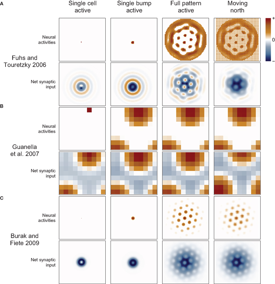
Figure 3. Synaptic connections play a major role in continuous attractor networks. For each of three 2D attractor models, we plot the activity of the sheet of neurons (top in each row) and the synaptic input to each cell caused by that activity (bottom in each row). (A) Each cell in the Fuhs and Touretzky (2006) model projects symmetrically outward in alternating rings of excitatory and inhibitory synapses. Just offset from the center, in this case downward, is an asymmetric inhibitory region (dark blue). When this cell fires, it inhibits the nearby cells except in a small region just above it where other cells are free to fire. Cells have different offset directions, so a bump of activity can form in a small group of cells that each inhibit a different direction around the bump, surrounding it in a ring of inhibition. All the cells here are driven to fire, creating new bumps spontaneously, and the excitatory ring surrounded by inhibition on each side encourages the new bumps to maintain a particular spacing. When the animal moves north, north-conjunctive cells increase in activity (producing the checker boarding of activity), increasing the inhibition on one side of each bump and causing the pattern to shift. (B) In Guanella et al. (2007) each cell has an identical synaptic output: an excitatory Gaussian bump that is inhibitory at long distances. The model has only one bump of activity, which wraps around on all sides, but with a “twist” in the up-down direction (see Figure 1A). The synapses change dynamically with velocity: e.g., when moving north the synaptic output is offset upward on the sheet of cells, which causes the bump to slide in that direction. (C) In Burak and Fiete (2009) the output of each cell is a ring of inhibition, the center offset in the direction the cell tries to move activity bumps (in this case offset two cells upward). The space inside the ring allows a bump to form, each active cell contributing to a strong ring of inhibition around the bump. The cells are driven to fire spontaneously so as many bumps form as is possible. Under the repulsive effects of the inhibitory rings, the bumps pack as tightly as possible, which is in a hexagonal grid. While moving north, north-conjunctive cells are driven strongly, slightly shifting the pattern of the synaptic drive and so shifting the bumps as well.
A more common and biologically plausible solution used in other grid cell models (O’Keefe and Burgess, 2005; Fuhs and Touretzky, 2006; McNaughton et al., 2006; Burak and Fiete, 2009; Navratilova et al., 2012) assigns a directional velocity input to some or all cells in the network, producing direction-conjunctive grid cells. The synaptic outputs of a conjunctive cell have a shift in a corresponding direction: the same or opposite direction, depending on whether the output is respectively excitatory (Navratilova et al., 2012) or inhibitory (Fuhs and Touretzky, 2006; Burak and Fiete, 2009), Figure 3. While standing still the velocity inputs to all cells are equal, so the synaptic output is symmetrical and the bump remains stationary. When velocity input increases to a subset of cells, their relative influence on the synaptic activity in the network increases, producing a momentarily biased network and allowing the network to path integrate. Two more-or-less equivalent variations of this mechanism are used: one simple arrangement (O’Keefe and Burgess, 2005; McNaughton et al., 2006; Navratilova et al., 2012) considers the pure grid cells as one population and assumes the existence of separate, parallel populations of conjunctive cells that are interconnected with the grid cells and responsible for shifting the pattern about. The other models (Fuhs and Touretzky, 2006; Burak and Fiete, 2009) do away with the pure grid cells and simply interconnect the conjunctive populations into one large network.
2.3. Read-Out
With the previously discussed mechanisms, an animal’s movements can be integrated into a running estimate of its position, and presumably this information is sent to many areas of the brain to support many processes, but our current interest is the way the information comes to appear as a hexagonal arrangement of spatial fields.
In Kropff and Treves (2008), the read-out mechanism is particularly simple: synaptic connections from place cells with fields arranged in a hexagonal grid directly drive a common grid cell.
In the 2D CAN models (Conklin and Eliasmith, 2005; O’Keefe and Burgess, 2005; Fuhs and Touretzky, 2006; McNaughton et al., 2006; Guanella et al., 2007; Burak and Fiete, 2009; Navratilova et al., 2012), the spatial grid pattern is a direct consequence of the positional code and no transformation is needed: the bump(s) of activity simply move in concert with the animal’s movements, and the networks are shaped so that bumps activate any given cell when the animal enters positions arranged in a hexagonal pattern.
The other models, however, break up the encoding of position into multiple networks, and these must be recombined with a read-out mechanism to produce the hexagonal field arrangement. Blair et al. (2007), for instance, stored a 2D position in multiple grid networks and, in a process of spatial interference, produced a larger scale grid pattern where the smaller grids overlap (Figure 1H). This is a planar-coding model, so the read-out is not needed to produce a 2D pattern per se, but rather to produce one of the necessary scale.
Read-out is mandatory, however, to produce a 2D hexagonal pattern in a linear-coding model. In such models the grid pattern is irrelevant to path integration and occurs as just one of many ways the encoded position may be read-out (Welday et al., 2011). Some models (Burgess et al., 2007; Gaussier et al., 2007; Hasselmo and Brandon, 2008; Mhatre et al., 2012) contain stripe or band cells (Figure 1G) that in 1D could look like repeating fields, but their firing pattern is clearly striped rather than a grid in 2D environments. However, when two or more of these patterns at 60° angles are overlaid, their intersections produce a 2D hexagonal grid. This is essentially the same process of spatial interference as in Blair et al. (2007). A natural neural implementation of spatial interference is given by the thresholded sum of inputs from the cells producing the stripes or grids (and see Figure 4).
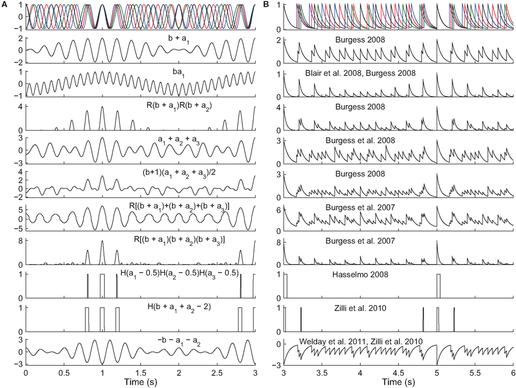
Figure 4. Read-out in temporal interference models. Top. A 5-Hz baseline oscillation (black) and three active oscillators (colors) path integrating while receiving a constant velocity input. The oscillator outputs are (A) sinusoids or (B) exponentially decaying synaptic potentials (50 ms time constant). The simulated animal begins between grid fields at time t = 0 s and enters fields at times t = {1,3,5} s. The remaining rows show the output of various models in response to the input oscillations (some using fewer than three active oscillator inputs). The rules all aim to produce maximal activity when the oscillators are all closely aligned in phase. The activity would then be thresholded (grid field width in vivo is about one-half the field spacing). Most of these rules were not intended to work with synaptic potentials (right column), but we show them to illustrate the difficulty of performing coincidence detection with spiking inputs: with some rules there is no threshold that would produce realistic field widths. Abbreviations: b, baseline oscillation; ai, active oscillations; H(x), the Heaviside step function (H(x) = 0 if x < 0 and H(x) = 1 if x ≥ 0), and R(x) the ramp function (R(x) = 0 if x < 0 and R(x) = x if x ≥ 0).
Temporal interference is another commonly used mechanism (Burgess et al., 2007; Giocomo et al., 2007; Blair et al., 2008; Burgess, 2008; Hasselmo, 2008; Zilli and Hasselmo, 2010; Welday et al., 2011). Whereas in spatial interference models, the grid cell inputs are either active or inactive at any time, in temporal interference models the inputs are always active (they fire at all locations) but their spike timing changes with respect to a baseline oscillation as a function of position. In these models the grid cell must become active when all of the inputs are sufficiently close in time to the baseline. In particular, grid field width is usually around one-half the field spacing, so the cell must fire when all active oscillators are within 90° of the baseline. Any mechanism that can perform this sort of coincidence detection will work. In the more abstract models (Burgess et al., 2007; Blair et al., 2008; Burgess, 2008; Hasselmo, 2008), various combinations of multiplying, adding, and thresholding the various inputs have been used successfully (Figure 4). A more realistically modeled grid cell must spike to reflect coincidence detection of its synaptic inputs, which can be can be difficult to carry out over an extended window with three or more inputs (two active and one baseline inputs). A simple approach (Zilli and Hasselmo, 2010; Welday et al., 2011) is to use inhibitory connections from the oscillators to the grid cell, and to drive the grid cell so it spikes spontaneously when not inhibited. The result is that when the oscillators are not sufficiently similar in phase, the grid cell receives tonic inhibition (Figure 4, bottom), but when the oscillators move into phase with each other, the grid cell is able to spike in the time between volleys of inhibition.
2.4. Learning
All of the grid cell models require specifically structured connectivity. Depending on the model, the connections may include: connections from specific directional velocity inputs to specific oscillators or cells, from specific oscillators or place cells to specific grid cells, or connections among grid and direction-conjunctive cells. The models only work if the synaptic connections and weights are close enough to their optimal values (Zhang, 1996; Burgess et al., 2007), so some mechanism must exist that allows the necessary connectivity to be learned (though at least one model has been shown to be robust to high levels of noise in the weights; Conklin and Eliasmith, 2005).
The following subsections describe the mechanisms that have been suggested for learning connections from one region or cell type to another.
2.4.1. Velocity to network oscillators
When a ring attractor or population of phase-synchronized spiking cells acts as a velocity-controlled oscillator, each of the cells must develop the same preferred input direction, and this learning problem has not been addressed for either type of oscillator. Standard self-organization methods may work when the oscillator is a network of phase-synchronized cells, as the co-activity of the cells may cause them all to select the same direction (though this suggestion is untested). For ring attractors, though, the problem is compounded because not only must all the conjunctive cells for one direction learn the same directional preference, but cells conjunctive for the other direction must all learn the opposite preferred direction.
2.4.2. Velocity to planar CANs
The complexity of the velocity to direction-conjunctive cell problem just mentioned is most clear in 2D attractor models. To control the bump of activity, conjunctive cells in at least three directions (and more commonly four) are required. Because the synaptic outputs of the conjunctive cells are shifted in some direction (see below regarding learning those connections), those cells have both a velocity input direction and a synaptic output direction, and not only must all cells with the same output direction learn to prefer the same input direction, but cells with different output directions must learn to prefer consistent input directions. If the cells with output direction up all develop a preference for north velocities, then the down output cells must develop a preference for south velocities, and this further constrains the input preferences that left and right cells can have. This problem has not yet been solved.
2.4.3. Place cells to grid cells
In place-driven models (Kropff and Treves, 2008), no learning of velocity inputs is required. Instead the grid cells must develop connections from place cells whose fields are arranged in a hexagonal pattern. Kropff and Treves (2008) gave a solution to this problem that can be thought of in two stages. In the first stage, grid cells develop place fields surrounded by rings of inactivity, and in the second stage these fields shift around to minimize their distance from each other, which produces the hexagonal field arrangement (Figure 1C).
This behavior comes from the combination of the learning rule and grid cell dynamics in the model. Grid cells undergo an inactivating adaptation, so a steady input makes a cell fire at a high rate, then adapt down to a lower rate, then return to a high rate as adaptation inactivates. The place-to-grid learning rule, roughly, increases the strength of active synapses when the grid cell’s activity is high, but weakens active synapses when the grid cell’s activity is low. The place-to-grid synaptic weights begin with random values, so as the animal explores, a grid cell will receive enough input to fire at random places. The learning rule strengthens the synapses that started the firing (reinforcing the firing field), but as the animal continues to move and adaptation lowers the grid cell’s activity, synapses from subsequently active place cells will decrease in weight onto the grid cell. With repeated passes through a grid field, the learning rule reinforces the strongest cells and then weakens surrounding cells, carving out an area of inactivity around the field. As the animal continues, adaptation inactivates and place cell inputs can again be strengthened, encouraging fields to appear or stabilize at that distance. The time or distance it takes for adaptation to inactivate roughly sets the scale of the grid pattern in this model.
However, place cells randomly remap in new environments while grid cells appear to maintain consistent relative spatial phases to each other (Leutgeb et al., 2005; Fyhn et al., 2007), while this mechanism must slowly re-learn the grid pattern in each new environment the animal is exposed to, unless a large number of maps have all been pre-learned (Samsonovich and McNaughton, 1997). The adaptation is also based on fixed time constants in the model, so the grid cell spacing depends on the history of velocities an animal has experienced in an environment.
2.4.4. Directional integrators to grid cells
Linear-coding models (Burgess et al., 2007; Gaussier et al., 2007; Giocomo et al., 2007; Blair et al., 2008; Burgess, 2008; Hasselmo, 2008; Hasselmo and Brandon, 2008; Zilli and Hasselmo, 2010; Welday et al., 2011; Mhatre et al., 2012) only produce the classic hexagonal field arrangement if the displacement is integrated along directions at 60° increments. One possibility is that the directional integrators only exist at 60° or 120° angles. Gaussier et al. (2007) gave a self-organizing map for learning spatial phases in a simplified version of this case.
Alternatively, directional integrators may exist for many directions and the grid cells must somehow learn to prefer input from specific directional integrators at appropriate angles. Burgess et al. (2007) showed in preliminary simulations that a cell’s activity was highest if it received three inputs at angles producing a hexagonal grid, suggesting that this could be the basis for self-organization of the 60° directional inputs. Mhatre et al. (2012) gave a model of grid cells as a self-organizing map that does just that. Input to their grid cells came in the form of a set of stripe cells (Figure 1G), which fire spatially in parallel lines of constant spacing but with systematically varied phases and directions. In their model the amount of plasticity increases with the activity level of the grid cell, and these stripe cell inputs compete for a limited total synaptic weight onto each grid cell. As a result, input patterns that occur frequently and produce the highest level of activity use up the most of the available synaptic weights, and Mhatre et al. (2012) argued geometrically that these inputs will be near 60°. Simulations show this mechanism produces fairly grid-like firing patterns, though the orientation of each cell in the network is not identical, in contradiction to the pattern observed in vivo. As this mechanism is experience-dependent, the grids develop slowly and require extended exposure to environments larger than the largest scale of the grids present in an animal’s brain for the grid to properly develop. Like the Kropff and Treves (2008) model, this mechanism is also velocity-dependent.
2.4.5. Grid cells to grid cells
When encoding position in attractor networks, synaptic connections among the grid and direction-conjunctive cells are needed to both maintain and update the pattern of activity. As suggested above, conjunctive cells must not only learn to prefer a common input direction, but their output must be directed to cells offset in a corresponding direction. A useful starting point may be analogous learning mechanisms used in head direction network models (Hahnloser, 2003; Stringer and Rolls, 2006).
In some models (Fuhs and Touretzky, 2006; McNaughton et al., 2006; Guanella et al., 2007; Navratilova et al., 2012), additional, symmetric synaptic connections are used to establish and maintain the pattern of activity. Fuhs and Touretzky (2006) gave a developmental model for learning the Mexican-hat–like connectivity shown in Figure 3. In their model, packets of activity randomly flowed over the network (by analogy with retinal waves in the developing eye). These packets were shaped like a sinusoidal grating, with alternating peaks of excitation and inhibition where the distance between peaks of excitation was the desired spacing of the rings in the synaptic matrix. Burak and Fiete (2006) reported that the symmetry of this Mexican-hat shape means it can maintain a grid at any orientation, so unfortunately the network has a tendency to drift in orientation.
McNaughton et al. (2006) suggested a mechanism that could solve this rotation problem, where the cells were directly connected to other cells hexagonally arranged in the sheet of cells, rather than having rotationally symmetric synaptic output in the form of rings. They showed that if entorhinal cells were driven by a sheet of cells with a drifting (in position but not rotation) hexagonal pattern of spiking, associative plasticity would connect co-active entorhinal cells into a toroidal topology, though Burak and Fiete (2006) reported this mechanism fails because the undesired rotations do occur.
2.5. Models
Having reviewed the individual components used in the models, we now briefly discuss each of the models themselves (summarized in Tables 1 and 2). The models are separated into linear- and planar-coding categories, because these two strands seemed to develop rather independently. Further technical details can be found in the comments in our online implementations of these models or in the papers themselves.
2.5.1. Linear-coding
O’Keefe and Burgess (2005), though focused on CAN models, called attention to earlier models that produced place cell theta phase precession through interfering oscillators (O’Keefe and Recce, 1993; Lengyel et al., 2003; Huhn et al., 2005). These models produced a series of equally spaced place fields, providing a fruitful starting point for later models.
Burgess et al. (2007) described subsequent work that generalized those models to two dimensions. In the basic temporal interference model, one grid cell received inputs from (or contained all of) the active oscillators, reading out the grid pattern in its activity. The main focus was on one biological implementation where LFP theta provided the baseline oscillation to a neuron’s soma, while SMPOs in the dendrites acted as active oscillators.
Giocomo et al. (2007) simulated a variant of the Burgess et al. (2007) modified to be consistent with their in vitro data (but see Burgess et al., 2007) showing that the resonant frequency and peak subthreshold membrane potential oscillation (SMPO) frequency of entorhinal cortical layer II stellate cells decreased in a dorsal to ventral gradient. In this model the baseline frequency scaled the speed inputs, so a lower frequency produced larger field spacing. As in Burgess et al. (2007), SMPOs were suggested to be the biological form of the model’s oscillators, but SMPOs within a cell cannot store arbitrary phase differences (Remme et al., 2009), and if they could, SMPOs are far too irregular to store one for long enough to create a stable grid (Welinder et al., 2008; Zilli et al., 2009; Dodson et al., 2011).
In Gaussier et al. (2007), linear positions were first encoded in the firing rates of two cells with preferred directions 60° apart. By integrating respective directional velocities, their activities gave the total displacement along the respective directions. The firing rate of these cells was discretized in a separate population E, e.g., one cell in E fires only when the animal has moved 10 cm in the x direction from its starting x coordinate (like stripe or band cells, except these have only a single band rather than repeating bands). E cells with firing bands at equal increments were synaptically connected to a modulo cell which then fired in a set of equally spaced parallel stripes. Finally, grid cells were created by adding or multiplying the activity of one modulo cell from each of the two directions. They also gave a simple learning mechanism that allowed grid cells to select a unique input from each of six different modulo populations at 60° increments. The learning was fairly trivial, however, creating a new grid cell for each novel combination of modulo cell activities experienced by the animal.
Blair et al. (2008) used temporal interference to read out linear positions stored between biased ring attractors rather than abstract, sinusoidal oscillators. The authors examined the firing phases of various cells in the network and found some cells precess (their Figures 4B,C show less than 180° of precession, not the 360° claimed) with respect to a baseline oscillation while other pairs of cells could show procession, shifting phases, or phase locking. Only the 1D case was modeled, the 2D case later appearing in Welday et al. (2011).
Burgess (2008) expanded on the Burgess et al. (2007) model, still using frequency-modulated sinusoids to perform path integration (also considering a slightly more spike-like shape from transforming the sinusoids), and examined the behavior of the model using various read-out mechanisms. He emphasized the importance of the baseline oscillation in reducing out-of-field spatial firing when oscillations are summed rather than multiplied. He also gave the first temporal interference model of grid cell phase precession that always precessed on every pass through a field. The precession mechanism used six oscillators at 60° increments: their frequencies increased or decreased normally, but at any time only the three oscillators that were firing faster than baseline were allowed to influence (through an unspecified mechanism) the grid cell, which then always fired faster than the baseline and so precessed.
Hasselmo (2008) gave a variation on the Burgess et al. (2007) model that interpreted the oscillator outputs as trains of spikes, represented artificially by thresholding a sinusoidal oscillation into a train of rectangular pulses. The model still path integrated through frequency modulation, but it did not use a baseline oscillator. The role of the baseline oscillator was played by an additional active oscillator along a third direction. Just as with a baseline oscillation, the third oscillator only moved into phase with the two others at positions arranged hexagonally. The lack of a baseline oscillation means that the model does not produce correct phase precession (and see Figure 7A left in Burgess, 2008). This paper also considered how place-based resetting of the grid system could explain context-dependent firing in the hippocampus and the non-grid pattern observed from grid cells in the hairpin maze (Derdikman et al., 2009), giving resetting mechanisms that would work with any path integration model.
Hasselmo and Brandon (2008) discussed multiple models including a spatial interference model they called a cyclical persistent firing model. Linear position was encoded in the firing rate of an individual cell, and that cell’s velocity input caused the firing rate to cycle such that the cell’s spatial firing occurred in parallel bands across the environment. In essence this is a temporal interference model with a baseline frequency of 0 Hz (like a single-cell analog of the cells found in a ring attractor), but it assumed an unspecified mechanism by which a constant input could modulate a cell’s firing rate in a sinusoidal manner.
Mhatre et al. (2012) addressed the issue of learning velocity inputs at 60° or 120° increments. They gave a self-organizing map (Grossberg, 1976a,b) receiving inputs in the form of increased activity along parallel lines at various orientations (their stripe cells, but possibly also Turing stripes, McNaughton et al., 2006, or band cells, Burgess et al., 2007) that could select for inputs at 60° increments and so eventually produce grid cells. The learning, however, produces grid cells at various orientations instead of one common orientation, seems to be sensitive to the velocity of the training trajectory, and requires early experience in large environments to learn the large-scale grids.
Zilli and Hasselmo (2010) addressed another concern in temporal interference models: the biological oscillators (SMPOs, LFP, and neuronal inter-spike or inter-burst intervals) considered in earlier models are highly noisy, which prevents them from stably storing a position on behavioral time scales (Welinder et al., 2008; Zilli et al., 2009). Zilli and Hasselmo (2010) showed that connecting a large enough number of cells in each oscillator allowed the synchronizing effect of coupling to overcome the independent noise injected into each cell. This produced spatial grid patterns that were fairly stable on the order of minutes, though such a large number of cells were needed as to seem wasteful. Other issues likely to recur in other increasingly biophysical interference grid cell models were discussed, including a lagging frequency response of neuronal oscillators, the non-linear frequency response of spiking neurons, and the difficulty performing coincidence detection on three or more inputs (especially when their magnitudes change stochastically). However, use of inhibitory inputs from oscillators (Figure 4) made coincidence detection easier (later confirmed by Welday et al., 2011).
Welday et al. (2011) continued the work of Blair et al. (2008), showing how arbitrary spatial firing patterns (including many seen in the medial temporal lobe) can be created by combining the outputs of biased ring attractors. They provided a valuable theoretical approach (carrying on from Blair et al., 2008) that focused on the spatial envelope of the interference of two oscillators, allowing questions of temporal interference to be treated as simpler spatial interference problems.
2.5.2. Planar-coding
Early path integration models that considered or used single-bump toroidal CANs (Zhang, 1996; Samsonovich and McNaughton, 1997) recognized that the place fields produced by the network would repeat as a rectangular grid in large environments, and the relationship between this pattern and grid cells was quickly noticed (Hafting et al., 2005).
Conklin and Eliasmith (2005) gave such a toroidal (rectangular grid) CAN and was the first modeling work to link it to the firing patterns of cells that would later be called grid cells (Fyhn et al., 2004; Hafting et al., 2005). This model featured improvements over earlier 2D CAN place cell models such as requiring fewer cells and tolerating heterogeneity in the cells and errors in the weight matrix.
Fuhs and Touretzky (2006) described a planar CAN model producing a hexagonal pattern of multiple bumps that could be moved over a circular sheet of cells. The rate-based grid cells were connected to nearby cells with concentric rings of excitatory and inhibitory synapses (Figure 3). With this pattern of connectivity, bumps of activity formed in a hexagonal pattern where the excitatory bands intersect (Figure 3). A conjunctive cell’s asymmetric output was an inhibitory region near the center of the concentric rings, offset opposite the direction that the cell would shift the population (each cell has one of four preferred directions). The recurrent weights faded out to 0 toward the edge of the network to prevent bumps of activity from forming lines parallel to the edges, creating cells at the edge that were barely spatially modulated and resembled head direction cells. Fuhs and Touretzky (2006) also described a developmental mechanism to learn the concentric rings component of the synaptic weights inspired by retinal waves observed in the developing eye. Later simulations (Burak and Fiete, 2006) showed that, due to uncontrollable rotations of the spatial pattern and a non-linear velocity response, this model fails to produce a stable spatial hexagonal grid.
McNaughton et al. (2006) further discussed the use of attractor dynamics, reviewing the basic functioning of ring and planar attractor networks (see also Zhang, 1996; Eliasmith, 2005). Their preliminary simulations (no details given) dealt with the problem of learning the toroidal synaptic connections needed for a single-bump 2D CAN like the one outlined in O’Keefe and Burgess (2005). McNaughton et al. (2006) reasoned that grid pattern development must be experience-independent because lab rats are unlikely to have been exposed to environments larger than the ventral grid spacing (a challenge to experience-dependent models like Kropff and Treves, 2008; Mhatre et al., 2012).
Blair et al. (2007) formed the hexagonal spatial pattern through spatial interference. Assuming the existence of small-scale, planar-coding “theta grids” (generated through unspecified attractor dynamics), they showed two ways two small-scale grids could interfere to produce the large-scale grid pattern (one hinted at in Figure 6A in McNaughton et al., 2006). By scaling-up or rotating one of the theta grids, its firing peaks would respectively phase precess or maintain a relatively fixed relationship with the fields of the other theta grid. If the spiking of one theta grid produced the LFP theta rhythm, spikes from the other grid could precess relative to theta. Blair et al. (2007) suggested this could relate to the difference between the theta phase profiles of cells in different layers of entorhinal cortex (Hafting et al., 2008). With this mechanism theta frequency would vary linearly with running speed, so they had to assume that the spacing of the grid producing LFP theta would vary with speed to keep theta frequency nearly constant. Consequently, the second grid had to dynamically scale or rotate to account for the changes in the first grid to maintain constant spacing in the large-scale grid.
Guanella et al. (2007) gave the first planar CAN model that produced a stable hexagonal spatial firing pattern. No conjunctive cells were used to update the stored position. Instead, the recurrent connections changed dynamically to shift the bump of activity smoothly and perfectly in any direction. The mechanism is conveniently simple, but not particularly biologically plausible. The authors introduced a twisted-torus topology to remedy the rectangular pattern produced by previous toroidal proposals (Conklin and Eliasmith, 2005; O’Keefe and Burgess, 2005; McNaughton et al., 2006). A twist in the torus is not strictly necessary: a hexagonal pattern results from an untwisted torus if the velocity input directions of certain conjunctive cells are skewed relative to their synaptic output directions (see online code). For example, the cells shifting the activity left and right still receive east and west velocity inputs, but the cells shifting the activity up and down receive velocity input along a direction 60° from the east/west direction (rather than the expected 90°). This modification produces elliptical rather than circular fields (a different solution to the toroidal problem is given by Burak and Fiete, 2009).
Kropff and Treves (2008) described a model that relied on place cell inputs rather than path integration. Their focus was on a developmental model that allowed a grid cell to develop its spatial pattern by slowly learning to prefer inputs from place cells whose fields are arranged in a hexagonal pattern. As described, the model produced grid cells that vary in orientation (unlike neighboring grid cells in vivo which appear to have the same orientation, Hafting et al., 2005). Also, distinct environments have distinct place field maps (Thompson and Best, 1989), so grid pattern would have to be relearned in each new environment, which is contrary to experimental reports that the grid pattern appears immediately on entry to a new environment (Hafting et al., 2005).
Burak and Fiete (2009) gave a multi-bump planar CAN, building on the work of Fuhs and Touretzky (2006) and Guanella et al. (2007), and studied many problems that can occur in this type of model. Their main focus was on the effects of periodic (i.e., toroidal) versus aperiodic (the network fades out to the edges which do not wrap around) networks. Edges produced detrimental effects in their aperiodic network, including noise-induced rotations of the pattern and inaccurate responses of the network to low velocity inputs. Fading out the velocity inputs to cells at the edges of the network (rather than fading out the synaptic weights as in Fuhs and Touretzky, 2006) lessened these effects. Those distortions also decreased in larger networks, so their large network with faded inputs path integrated successfully. Periodic networks, having no edges, had none of these problems, though finer tuning of the grid spacing was required so that the pattern perfectly fit the dimensions of the sheet of cells. The authors also showed that an attractor network of stochastically spiking cells is considerably more robust to small amounts of noise than models (Burgess et al., 2007; Gaussier et al., 2007; Giocomo et al., 2007; Burgess, 2008; Hasselmo, 2008; Hasselmo and Brandon, 2008) where only a single noisy cell encodes position (and see Zilli et al., 2009).
Navratilova et al. (2012) extended CAN models to address theta phase precession, focusing on the 1D case. The model included an 8 Hz theta oscillation injected into the conjunctive cells and an artificial ADP and mAHP injected into the grid cells after a spike. The grid cells formed an unbiased ring attractor and projected to corresponding cells in the conjunctive populations (6 o’clock grid cells to 6 o’clock conjunctive cells). The two populations of conjunctive cells projected back to the grid cells, but offset in each direction. Thus an input from one spiking grid cell drove activity in the conjunctive populations at the same position, which drove grid cells on either side of the first grid cell. Biased by velocity input, one conjunctive population has greater activity, asymmetrically driving the grid cells and nudging the bump in one direction. When the newly active grid cells fire, the cycle repeats and the bump continues moving. The ADP, mAHP, and NMDA time constants in the grid cell determine how quickly the grid cell bump can re-fire, setting how many times the bump can nudge forward in any unit of time, and so influencing grid field spacing. This process occurs with the conjunctive cells depolarized to near threshold by the theta input, but at the trough of the theta input, the conjunctive cells fire much less. At those times the ADP currents of recently active grid cells caused them to fire again, making the bump of activity jump back to an earlier point. Theta phase precession arises from this alternation of the bump moving forward under the influence of velocity followed by the bump jumping back. Only a 1D version of the model was given, but the model might be extended to 2D either via spatial interference of two rings or by expanding it to be a planar-coding CAN (Guanella et al., 2007; Burak and Fiete, 2009).
3. Discussion
3.1. Summary
Rather than the common division of continuous attractor vs. interference models, we suggest alternative categorizations.
The positional codes in the models fall into linear-coding and planar-coding categories. The key difference is that linear-coding models independently encode linear positions along different directions such that changing the position encoded along one direction may not affect encoded positions along other directions. In planar-coding models, although individual cells have preferred directions, the position coded by the set of cells with one preferred direction is also changed by movements along any other direction. The models can also be distinguished according to the mechanisms used to encode and maintain positions. Unbiased attractor networks or oscillator phase differences are most commonly used, though some models use more direct positional codes like place cells or encoding coordinates as firing rates.
A more fine-grained, but non-exclusive categorization of the models is given by the mechanism used to update the encoded position. Positions stored using abstract oscillators or phase-synchronized spiking cells are updated by modulating the frequency or firing rate of the oscillators, and positions stored in unbiased continuous attractor networks are updated through direction-conjunctive cells. Biased attractor networks, however, can be understood as both: inputs modulate the frequency of the networks, but this is done via conjunctive cells.
Finally, the models can be categorized by their read-out mechanisms, a distinction loosely related to the linear vs. planar distinction. Planar models do not generally require a read-out mechanism to produce a 2D grid (but see Blair et al., 2007), while read-out mechanisms are required for linear-coding models. For simplicity we divided the read-out mechanisms into temporal interference and spatial interference, though they are essentially equivalent because temporal interference models become spatial interference models when the baseline oscillation frequency is set to 0 Hz.
3.2. Experiments and Models
The publications we have reviewed all give models on Marr’s algorithmic level (Table 1), and many also specify an implementation (Table 2). The two levels have different values and uses.
On the algorithmic level, simulations have theoretical value as proofs-of-concept demonstrating that a solution can actually work, but these make fairly limited experimental predictions regarding only phenomena that might be observed. For example, algorithmically Burgess et al.’s (2007) model can only predict that somewhere in the brain there are oscillatory processes being modulated by the animal’s body velocity. Similarly, Burak and Fiete’s (2009) model can only predict that somewhere there are velocity-sensitive (i.e., conjunctive) grid cells whose gain changes when an environment is deformed or which always maintain a perfect spatial phase relationship.
This limitation arises because a single algorithmic model or prediction can have many different biological implementations and experiments can only directly support or oppose specific implementational predictions. For example, spatial position in CAN models should be perturbed if the direction-conjunctive cells are perturbed, but some cells may inherit the direction signal without partaking in network dynamics and perturbing such a cell may have no effect. That null result should not be evidence against the algorithmic model, but would be evidence against a particular implementation.
As a result, the valuable experimental predictions of a model generally come from the implementational level where specific properties are attributed to specific anatomical or electrophysiological elements. This is a valuable step because predictions become concrete and easily tested, though there is a degree of arbitrariness in selecting an implementation and only this arbitrary implementation can actually be evaluated (rather than the algorithmic model itself).
Temporal interference models that include theta-rhythmic (spiking or subthreshold oscillations or external input modulated at a theta frequency) elements provide one example of the value of distinguishing among these levels.
There are many oscillatory processes in the rodent medial temporal lobe that show rhythmicity in the 6 to 10 Hz theta band, including fluctuations in the local field potential (LFP), subthreshold fluctuations in neuronal membrane potentials, and bursting or modulation of firing rate of many cells types (and so also rhythmic synaptic input to cells over recurrent connections). The prominence of these oscillations has led to their use in many implementation-level models that have made explicit predictions about how the scale of the grid pattern may be reflected in rhythmic processes (O’Keefe and Burgess, 2005; Burgess et al., 2007; Burgess, 2008). Many predictions have been confirmed (Giocomo et al., 2007; Giocomo and Hasselmo, 2008; Jeewajee et al., 2008; Welday et al., 2011; Navratilova et al., 2012). At the same time, experimental (Welinder et al., 2008; Zilli et al., 2009; Dodson et al., 2011) and theoretical (Remme et al., 2009, 2010) arguments have been raised against the same implementations.
Recently Yartsev et al. (2011) provocatively claimed to have disproven the entire class of “oscillatory interference” models based on the fact that the LFP in bats contained no strong theta signal nor did the grid cells show theta modulation in their spike time autocorrelations. If theta is the same frequency in bats as rats (though the functional role, not the numerical frequency value is what is important in the models), this would be good evidence against an implementation that involves theta, but no more evidence against the whole class of interference models than any of the earlier experimental results identifying flaws in those implementations. Algorithmically, no model requires any regular rhythmic components nor necessarily produces them as output (see our online code; although the bat data seems to contain a low frequency rhythmic component around 1/3–1 Hz that would still be consistent with the temporal interference models).
The interesting result of making explicit predictions is that models that make them have been quite successful in guiding experiments that have discovered new results, and the experiments have been quite consistent in revealing flaws with the originally specified implementations.
3.2.1. Distinguishing linear from planar-coding
It is natural to ask how experiments might distinguish linear- from planar-coding models. A direct approach would be a time consuming, systematic search for linear coding (either cells with stripe-like firing patterns or oscillators whose phase relative to a baseline varies with directional position) in the inputs to grid cells. Locating such a code would provide great support to linear-coding models, though the challenge would remain to show those inputs are in fact used to create the grid.
Alternatively, the effects of linear-coding inputs may be visible in intracellular recordings of grid cells in vivo. The linear position inputs may be fairly strong because few such inputs are required in these models (though out-of-field inputs might be hidden by dendritic non-linearities). Spatial interference models predict strong, tonic subthreshold inputs at positions along the lines between adjacent fields, but not in the central spaces of triangles of fields. Temporal interference models predict grid cells should receive multiple inputs (modulated around a common baseline frequency) with relative phases that vary systematically with position, and subsets of these should move into alignment at positions along the lines connecting adjacent fields (Figure 4).
These predictions are in contrast to planar-coding models, where there might be spatially correlated (e.g., sensory) subthreshold inputs or even inputs that repeat systematically with the grid (e.g., from flaws in a synaptic weight matrix), but most models would not predict consistent inputs only along lines of a particular orientation connecting adjacent fields. One exception is the Fuhs and Touretzky (2006) model, which contains cells near the network edge that might produce such stripe-y grid cells if the model accurately path integrated. Though the case of subthreshold inputs may be easier to detect, in vivo intracellular recording is still in its infancy, so these predictions might also be examined in the positions of out-of-field grid cell spiking (i.e., out-of-field firing primarily along lines connecting neighboring fields may suggest linear-coding).
The linear/planar distinction, however, should not be thought of as necessarily intrinsic to a model. In theory any of the planar-coding CAN models could be reduced down to a ring attractor and a pair used in a linear-coding model. Linear-coding approaches can also be merged into a planar code (e.g., an unbiased ring attractor where the bump position indicates spatial position along one direction and the phase relative to a baseline of bursts of bump activity encodes position along a second direction).
3.2.2. Questions for future work
A number of questions about grid cells arise from studying the models in detail.
First, path integration requires the body’s movements as inputs, but the grid cell literature largely focuses on the existence of head direction cells in the medial temporal lobe. Do head direction cells actually encode body movement direction, or, if not, do path integration errors consistently occur if the animal moves forward with its head rotated to one side? Also, when a grid cell has a directional preference, is the preference always along a direction connecting adjacent fields (and if so, along three or all six directions?) or are all directions represented?
Grid cells often show firing at positions along environmental edges that does not conform to the overall hexagonal pattern. Though grid cell models allow for sensory inputs on the grid cell, no model specifically tries to explain this edge firing. In particular, if the regularity of grid fields is key to the use of grid cells as a spatial code, are spatial abilities impaired at environmental boundaries?
It has sometimes been suggested that local flaws in grid field spacing can create pentagons or heptagons rather than hexagons (Fuhs and Touretzky, 2006). Does this actually occur or is it due to edge effects or undersampling of animal positions? If it does occur, are spatial abilities impaired in environments where it is observed?
Is the amount of phase precession observed within a field correlated with the ratio of field width to field spacing? Temporal interference models predict that firing phase range is 360° · (field width)/(field spacing). This phase range applies only to the range where the spikes are truly precessing, not the second component (Yamaguchi et al., 2001) as the animal exits the field, where the cell fires across most phases.
Are grid fields firmly established immediately on entry into a new environment and does a grid cell always fire on every pass through each field? Both during the course of development and on exposure to a novel environment, do dorsal grid cells appear or stabilize before ventral grid cells? Experience-dependent learning models must reform the grid pattern in new environments, but they might be able to more quickly organize grid cells with smaller field spacing.
In the event that the environment is stretched or deformed such that place cells stretch their place fields, the grid pattern would also be expected to stretch or deform to match (Blair et al., 2007; Burgess et al., 2007). A stretched grid pattern due to place influences can be distinguished from a stretched grid due to changes in input gain along different directions (an alternative explanation) by comparing the velocity-modulation and firing fields of pairs of simultaneously recorded grid cells (Burak and Fiete, 2009).
Does a grid cell’s firing rate slow down in the middle of a field? Models like Kropff and Treves (2008) and Mhatre et al. (2012) require adaptation or habituation dynamics that decrease the activity of tonically active cells.
3.3. Attractors and Interference
A common division of grid cell models is into continuous attractor network and oscillatory interference models. As we have already suggested, this distinction is misleading because it contrasts independent qualities. To distinguish their general meanings from the classes of models the terms have come to represent, additional points about attractors and interference are worth mentioning.
An attractor is a state (or region of state space) that a system moves toward if the system’s state is nearby. All neurons have attractors: both the stable equilibrium of a neuron at rest and the consistent voltage trajectory (limit cycle) maintained by a steadily spiking cell are attractors. A system can have multiple simultaneous attractors: bistable cells can have both a resting equilibrium and a spiking limit cycle at the same time, and others (Hughes et al., 1999; Izhikevich, 2007) have two simultaneously stable voltage attractors (e.g., with no applied current, the voltage can remain at −75 or at −59 mV, and brief inputs can move it back and forth). A system can even have infinitely many attractors (e.g., a hypothetical cell that could stably maintain any voltage in between −75 and −59 mV). This is called a continuous attractor (continuous meaning there is always a third attractor between any two nearby attractors). A similar continuous attractor is used in Gaussier et al. (2007) and Hasselmo and Brandon (2008) in their cells that store a coordinate in their firing rates. Similarly, networks of cells have attractors, and such networks are called attractor networks when the attractor aspect is emphasized. The phase-synchronized state of a population of cells can be an attractor (Izhikevich, 2007), so Zilli and Hasselmo (2010) used (non-continuous) attractor networks in their model. Continuous attractors can also occur in networks, as in the many ring and 2D attractor models described above. In these the attractors are patterns of neural activities containing one or more localized bumps. Continuous attractor networks are less generic than other attractors since they require patterned synaptic connections, but as Conklin and Eliasmith (2005) showed, imperfect networks can behave as CANs. The CAN metaphor is thus a matter of degree, not a binary property of a system.
Interference refers to the signal produced by combining two other signals, with emphasis on the large peaks in the output where the inputs constructively interfere and the low points where the inputs are out of phase and destructively interfere. This is not a special mechanism, but rather a simple physical fact that two inputs to a cell that co-occur will produce a larger net effect than if they had occurred separately. Even in planar CANs, each conjunctive cell has a slightly different synaptic output pattern and the final activity of the cells is given by the sum of all of these patterns, producing a sort of synaptic spatial interference [e.g., in Fuhs and Touretzky (2006), the arrangement of bumps is the interference pattern of the synaptic rings of excitatory and inhibitory outputs]. In grid cell models, the term oscillatory interference is generally used, suggesting more specifically the interference of regular oscillations (presumably temporal or spatial) rather than simply identifying the overlap of multiple synaptic inputs, but any signal can be considered a complex oscillation in some sense.
Attractors and interference appear not only in the grid cell models named after them, but also in the other grid cell models, and are general properties of every circuit in the brain. This is clear from their widespread occurrence in other models. For example, a focus on interference of oscillations arose in models of place cell precession (O’Keefe and Recce, 1993; Lengyel et al., 2003; Huhn et al., 2005; O’Keefe and Burgess, 2005), but also, e.g., models of timing (Miall, 1989; Hopfield and Brody, 2001). Attractor networks have been used to model both place cells (Samsonovich and McNaughton, 1997; Conklin and Eliasmith, 2005) and head direction cells (Skaggs et al., 1995; Zhang, 1996), and many other systems (Eliasmith, 2005).
3.4. Noise
As path integration models require that a position be both stably encoded and accurately updated, successful models must account for the high levels of noise observed in biological systems. All of the path integration models are equally susceptible to noise in the velocity inputs themselves (Burak and Fiete, 2009; Zilli et al., 2009), so the noise intrinsic to the system is most commonly studied. Noise is also assumed to have a mean of zero, as non-zero mean noise introduces a constant bias that strongly disrupts the stable grid pattern (Giocomo and Hasselmo, 2008).
Early models encoding positions as phase differences were considered particularly susceptible to noise (Burgess et al., 2007; Giocomo and Hasselmo, 2008; Hasselmo, 2008; Welinder et al., 2008), though later work showed that the use of multiple, redundant oscillators allowed for robustness to small levels of noise (Zilli et al., 2009). Considerably greater robustness to noise was provided by subsequent work in which each oscillator comprised many coupled spiking neurons (Zilli and Hasselmo, 2010).
This is a general effect of coupled cells, so all CANs automatically attain robustness to noise (including those used to encode phase differences; e.g., Blair et al., 2008). Burak and Fiete (2009) examined the behavior of CANs with intrinsic noise and showed that toroidal networks are robust to noise, with the pattern drifting in a diffusion process, while aperiodic networks were less robust, showing the same translational diffusion but also a more damaging rotational drifting of the pattern. The same diffusive process producing error in the encoded position occurs with noise in phase difference models (Zilli et al., 2009), suggesting it is likely the generic behavior of path integration models with internal noise. To deal with the drifting pattern that occurs with noise, Guanella et al. (2007) simulated connections from place cells to grid cells that could reset the grid network. Navratilova et al. (2012) showed that phase precession in their model was also robust to the presence of noise.
3.5. “Best” Model
It is possible exactly one current model or mechanism fully explains the grid pattern to the complete exclusion of all other models or alternative mechanisms, but grid cells are part of a messy biological system created through natural selection and individual development. Grid cell models are designed specifically to produce the grid in as simple a manner as possible, but the biological system is unlikely to have evolved with the goal of finding the simplest way to produce a grid. Grid cells individually or as a population likely perform a complex and perhaps context-sensitive processing on inputs that may themselves reflect various complex, context-sensitive mechanisms, and so the models may better be considered collectively as a set of metaphors that guide research by describing how grid cells may possibly be driven at various times or in different states, rather than as things to be proven or disproven. For example, the place-driven metaphor of Kropff and Treves (2008) may be true in familiar environments, and linear-coding or planar-coding used respectively in 1D or 2D environments, or perhaps both 1D and 2D environments are coded linearly, while incidental (e.g., standing on a moving platform or pushing against a wall and sliding backward) or illusory(e.g., the bus next to your car backs up slightly, creating the illusion of forward motion) movements might be understood as updating the position representation through conjunctive cells as in CANs.
These are meant as examples, not predictions, but it is easy to see that, given the variety of ways that spatial position could change, and the distinct systems that may encode or produce different types of movements, there is much room for a variety of mechanisms to be involved in the unitary representation of position that grid cells are thought to reflect.
Conflict of Interest Statement
The author declares that the research was conducted in the absence of any commercial or financial relationships that could be construed as a potential conflict of interest.
Acknowledgments
I thank Mark Brandon, Jason Climer, Michael Hasselmo, Jim Heys, Caitlin Monaghan, and Yusuke Tsuno for comments and discussion, and Yoram Burak, Stephen Grossberg, Michael Hasselmo, Himanshu Mhatre, Zaneta Navratilova, Praveen Pilly, and Bailu Si for discussions, information, and materials helpful in implementing various models. Supported by grants to Michael Hasselmo (ONR MURI award N00014-10-1-0936, NIMH Silvio O. Conte grant P50 MH094263, and NIMH R01 MH60013).
References
Blair, H. T., Gupta, K., and Zhang, K. (2008). Conversion of a phase- to rate-coded position signal by a three-stage model of theta cells, grid cells, and place cells. Hippocampus 18, 1239–1255.
Blair, H. T., Welday, A. W., and Zhang, K. (2007). Scale-invariant memory representations emerge from moiré interference between grid fields that produce theta oscillations: a computational model. J. Neurosci. 27, 3211–3229.
Brun, V. H., Solstad, T., Kjelstrup, K. B., Fyhn, M., Witter, M. P., Moser, E. I., and Moser, M.-B. (2008). Progressive increase in grid scale from dorsal to ventral medial entorhinal cortex. Hippocampus 18, 1200–1212.
Burak, Y., and Fiete, I. R. (2006). Do we understand the emergent dynamics of grid cell activity? J. Neurosci. 26, 9352–9354.
Burak, Y., and Fiete, I. R. (2009). Accurate path integration in continuous attractor network models of grid cells. PLoS Comput. Biol. 5, e1000291. doi:10.1371/journal.pcbi.1000291
Burgess, N. (2008). Grid cells and theta as oscillatory interference: theory and predictions. Hippocampus 18, 1157–1174.
Burgess, N., Barry, C., and O’Keefe, J. (2007). An oscillatory interference model of grid cell firing. Hippocampus 17, 801–812.
Burgess, N., O’Keefe, J., and Recce, M. (1993). “Using hippocampal ‘place cells’ for navigation, exploiting phase coding,” in Advances in Neural Information Processing Systems 5, eds S. J. Hanson, C. L. Giles, and J. D. Cowan (San Mateo: Morgan Kaufmann Publishers Inc.), 929–936.
Conklin, J., and Eliasmith, C. (2005). A controlled attractor network model of path integration in the rat. J. Comput. Neurosci. 18, 183–203.
Derdikman, D., Whitlock, J. R., Tsao, A., Fyhn, M., Hafting, T., Moser, M.-B., and Moser, E. I. (2009). Fragmentation of grid cell maps in a multicompartment environment. Nat. Neurosci. 12, 1325–1332.
Dodson, P., Pastoll, H., and Nolan, M. (2011). Dorsal-ventral organization of theta-like activity intrinsic to entorhinal stellate neurons is mediated by differences in stochastic current fluctuations. J. Physiol. (Lond.) 589, 2993–3008.
Eliasmith, C. (2005). A unified approach to building and controlling spiking attractor networks. Neural Comput. 17, 1276–1314.
Fuhs, M. C., and Touretzky, D. S. (2006). A spin glass model of path integration in rat medial entorhinal cortex. J. Neurosci. 26, 4266–4276.
Fyhn, M., Hafting, T., Treves, A., Moser, M.-B., and Moser, E. I. (2007). Hippocampal remapping and grid realignment in entorhinal cortex. Nature 446, 190–194.
Fyhn, M., Molden, S., Witter, M. P., Moser, E. I., and Moser, M.-B. (2004). Spatial representation in the entorhinal cortex. Science 305, 1258–1264.
Gaussier, P., Banquet, J. P., Sargolini, F., Giovannangeli, C., Save, E., and Poucet, B. (2007). A model of grid cells involving extra hippocampal path integration, and the hippocampal loop. J. Integr. Neurosci. 6, 447–476.
Giocomo, L. M., and Hasselmo, M. E. (2008). Computation by oscillations: implications of experimental data for theoretical models of grid cells. Hippocampus 18, 1186–1199.
Giocomo, L. M., Moser, M.-B., and Moser, E. I. (2011). Computational models of grid cells. Neuron 71, 589–603.
Giocomo, L. M., Zilli, E. A., Fransén, E., and Hasselmo, M. E. (2007). Temporal frequency of subthreshold oscillations scales with entorhinal grid cell field spacing. Science 23, 1719–1722.
Grossberg, S. (1976a). Adaptive pattern classification and universal recoding, II: feedback, expectation, olfaction, and illusions. Biol. Cybern. 23, 187–202.
Grossberg, S. (1976b). Adaptive pattern classification and universal recoding, I: parallel development and coding of neural feature detectors. Biol. Cybern. 23, 121–134.
Guanella, A., Kiper, D., and Verschure, P. (2007). A model of grid cells based on a twisted torus topology. Int. J. Neural Syst. 17, 231–240.
Hafting, T., Fyhn, M., Bonnevie, T., Moser, M. B., and Moser, E. I. (2008). Hippocampus-independent phase precession in entorhinal grid cells. Nature 453, 1248–1252.
Hafting, T., Fyhn, M., Molden, S., Moser, M. B., and Moser, E. I. (2005). Microstructure of a spatial map in the entorhinal cortex. Nature 436, 801–806.
Hahnloser, R. H. R. (2003). Emergence of neural integration in the head-direction system by visual supervision. Neuroscience 120, 877–891.
Hasselmo, M. E. (2008). Grid cell mechanisms and function: contributions of entorhinal persistent spiking and phase resetting. Hippocampus 18, 1213–1229.
Hasselmo, M. E., and Brandon, M. P. (2008). Linking cellular mechanisms to behavior: entorhinal persistent spiking and membrane potential oscillations may underlie path integration, grid cell firing and episodic memory. Neural Plast. 2008, 658323.
Hayman, R., Verriotis, M., Jovalekic, A., Fenton, A., and Jeffery, K. J. (2011). Anisotropic encoding of three-dimensional space by place cells and grid cells. Nat. Neurosci. 14, 1182–1188.
Hopfield, J. J., and Brody, C. D. (2001). What is a moment? Transient synchrony as a collective mechanism for spatiotemporal integration. Proc. Natl. Acad. Sci. U.S.A. 98, 1282–1287.
Hughes, S. W., Cope, D. W., Toth, T. L., Williams, S. R., and Crunelli, V. (1999). All thalamocortical neurones possess a T-type Ca2+ ‘window’ current that enables the expression of bistability-mediated activities. J. Physiol. (Lond.) 517, 805–815.
Huhn, Z., Orbán, G., Érdi, P., and Lengyel, M. (2005). Theta oscillation-coupled dendritic spiking integrates inputs on a long time scale. Hippocampus 15, 950–962.
Izhikevich, E. M. (2007). Dynamical Systems in Neuroscience: The Geometry of Excitability and Bursting. Cambridge, MA: MIT Press.
Jeewajee, A., Barry, C., O’Keefe, J., and Burgess, N. (2008). Grid cells and theta as oscillatory interference: electrophysiological data from freely moving rats. Hippocampus 18, 1175–1185.
Kalaska, J. F., Caminiti, R., and Georgopoulos, A. P. (1983). Cortical mechanisms related to the direction of two-dimensional arm movements: relations in parietal area 5 and comparison with motor cortex. Exp. Brain Res. 51, 247–260.
Kropff, E., and Treves, A. (2008). The emergence of grid cells: intelligent design or just adaptation. Hippocampus 18, 1256–1269.
Lengyel, M., Szatmáry, Z., and Érdi, P. (2003). Dynamically detuned oscillations account for the coupled rate and temporal code of place cell firing. Hippocampus 13, 700–714.
Leutgeb, S., Leutgeb, J. K., Barnes, C. A., Moser, E. I., McNaughton, B. L., and Moser, M.-B. (2005). Independent codes for spatial and episodic memory in hippocampal neuronal ensembles. Science 309, 619–623.
Marr, D. (1982). Vision: A Computational Investigation into the Human Representation and Processing of Visual Information. New York: Freeman.
McNaughton, B. L., Barnes, C. A., Gerrard, J. L., Gothard, K., Jung, M. W., Knierim, J. J., Kudrimoti, H., Qin, Y., Skaggs, W. E., Suster, M., and Weaver, K. L. (1996). Deciphering the hippocampal polyglot: the hippocampus as a path integration system. J. Exp. Biol. 199, 173–185.
McNaughton, B. L., Battaglia, F. P., Jensen, O., Moser, E. I., and Moser, M. B. (2006). Path integration and the neural basis of the ‘cognitive map’. Nat. Rev. Neurosci. 7, 663–678.
Mhatre, H., Gorchetchnikov, A., and Grossberg, S. (2012). Grid cell hexagonal patterns formed by fast self-organized learning within entorhinal cortex. Hippocampus 22, 320–334.
Miall, C. (1989). The storage of time intervals using oscillating neurons. Neural Comput. 1, 359–371.
Milford, M. J., Wiles, J., and Wyeth, G. F. (2010). Solving navigational uncertainty using grid cells on robots. PLoS Comput. Biol. 6, e1000995. doi:10.1371/journal.pcbi.1000995
Navratilova, Z., Giocomo, L. M., Fellous, J.-M., Hasselmo, M. E., and McNaughton, B. L. (2012). Phase precession and variable spatial scaling in a periodic attractor map model of medial entorhinal grid cells with realistic after-spike dynamics. Hippocampus 22, 772–789.
O’Keefe, J. (1976). Place units in the hippocampus of the freely moving rat. Exp. Neurol. 51, 78–109.
O’Keefe, J., and Burgess, N. (2005). Dual phase and rate coding in hippocampal place cells: theoretical significance and relationship to entorhinal grid cells. Hippocampus 15, 853–866.
O’Keefe, J., and Recce, M. L. (1993). Phase relationship between hippocampal place units and the EEG theta rhythm. Hippocampus 3, 317–330.
Redish, A. D. (1999). Beyond the Cognitive Map: From Place Cells to Episodic Memory. Cambridge, MA: MIT Press.
Remme, M. W. H., Lengyel, M., and Gutkin, B. S. (2009). The role of ongoing dendritic oscillations in single-neuron dynamics. PLoS Comput. Biol. 5, e1000493. doi:10.1371/journal.pcbi.1000493
Remme, M. W. H., Lengyel, M., and Gutkin, B. S. (2010). Democracy-independence trade-off in oscillating dendrites and its implications for grid cells. Neuron 66, 429–437.
Samsonovich, A., and McNaughton, B. L. (1997). Path integration and cognitive mapping in a continuous attractor neural network model. J. Neurosci. 17, 5900–5920.
Sargolini, F., Fyhn, M., Hafting, T., McNaughton, B. L., Witter, M. P., Moser, M. B., and Moser, E. I. (2006). Conjunctive representation of position, direction, and velocity in entorhinal cortex. Science 312, 758–762.
Skaggs, W. E., Knierim, J. J., Kudrimoti, H., and McNaughton, B. L. (1995). A model of the neural basis of the rat’s sense of direction. Adv. Neural Inf. Process. Syst. 7, 173–180.
Skaggs, W. E., McNaughton, B. L., Wilson, M. A., and Barnes, C. A. (1996). Theta phase precession in hippocampal neuronal populations and the compression of temporal sequences. Hippocampus 6, 149–172.
Stringer, S. M., and Rolls, E. T. (2006). Self-organizing path integration using a linked continuous attractor and competitive network: path integration of head direction. Network 17, 419–445.
Thompson, L. T., and Best, P. J. (1989). Place cells and silent cells in the hippocampus of freely-behaving rats. J. Neurosci. 9, 2382–2390.
Touretzky, D. S., Redish, A. D., and Wan, H. S. (1993). Neural representation of space using sinusoidal arrays. Neural Comput. 5, 869–884.
van Hemmen, J. L., and Schwartz, A. B. (2008). Population vector code: a geometric universal as actuator. Biol. Cybern. 98, 509–518.
Welday, A. C., Shlifer, I. G., Bloom, M. L., Zhang, K., and Blair, H. T. (2011). Cosine directional tuning of theta cell burst frequencies: evidence for spatial coding by oscillatory interference. J. Neurosci. 31, 16157–16176.
Welinder, P. E., Burak, Y., and Fiete, I. R. (2008). Grid cells: the position code, neural network models of activity, and the problem of learning. Hippocampus 18, 1283–1300.
Yamaguchi, Y., Aota, Y., McNaughton, B. L., and Lipa, P. (2001). Bimodality of theta phase precession in hippocampal place cells in freely running rats. J. Neurophysiol. 87, 2629–2642.
Yartsev, M. M., Witter, M. P., and Ulanovsky, N. (2011). Grid cells without theta oscillations in the entorhinal cortex of bats. Nature 479, 103–107.
Zhang, K. (1996). Representation of spatial orientation by the intrinsic dynamics of the head-direction cell ensemble: a theory. J. Neurosci. 16, 2112–2126.
Zilli, E. A., and Hasselmo, M. E. (2010). Coupled noisy spiking neurons as velocity-controlled oscillators in a model of grid cell spatial firing. J. Neurosci. 30, 13850–13860.
Keywords: medial temporal lobe, path integration, place cell, ring attractor, self-organization
Citation: Zilli EA (2012) Models of grid cell spatial firing published 2005–2011. Front. Neural Circuits 6:16. doi: 10.3389/fncir.2012.00016
Received: 10 December 2011; Accepted: 22 March 2012;
Published online: 18 April 2012.
Edited by:
Yasser Roudi, Norwegian University of Science and Technology, NorwayCopyright: © 2012 Zilli. This is an open-access article distributed under the terms of the Creative Commons Attribution Non Commercial License, which permits non-commercial use, distribution, and reproduction in other forums, provided the original authors and source are credited.
*Correspondence: Eric A. Zilli, Department of Psychology, Center for Memory and Brain, Boston University, 2 Cummington Street, Boston, MA 02215, USA. e-mail: zilli@bu.edu