Waiting is the hardest part: comparison of two computational strategies for performing a compelled-response task
- Department of Neurobiology and Anatomy, Wake Forest University School of Medicine, Winston-Salem, NC, USA
The neural basis of choice behavior is commonly investigated with tasks in which a subject analyzes a stimulus and reports his or her perceptual experience with an appropriate motor action. We recently developed a novel task, the compelled-saccade task, with which the influence of the sensory information on the subject’s choice can be tracked through time with millisecond resolution, thus providing a new tool for correlating neuronal activity and behavior. This paradigm has a crucial feature: the signal that instructs the subject to make an eye movement is given before the cue that indicates which of two possible choices is the correct one. Previously, we found that psychophysical performance in this task could be accurately replicated by a model in which two developing oculomotor plans race to a threshold and the incoming perceptual information differentially accelerates their trajectories toward it. However, the task design suggests an alternative mechanism: instead of modifying an ongoing oculomotor plan on the fly as the sensory information becomes available, the subject could try to wait, withholding the oculomotor response until the sensory cue is revealed. Here, we use computer simulations to explore and compare the performance of these two types of model. We find that both reproduce the main features of the psychophysical data in the compelled-saccade task, but they give rise to distinct behavioral and neurophysiological predictions. Although, superficially, the waiting model is intuitively appealing, it is ultimately inconsistent with experimental results from this and other tasks.
1 Introduction
To pick the tastiest strawberry from a plate, one looks at their colors, shapes, sizes, how soft, or hard they are, and so on. In analogy with this type of everyday-life situation, to study how choices are made, a common strategy is to present a simplified sensory scene and investigate how its perceptual analysis leads to one of two or more possible motor responses (e.g., Shadlen and Newsome, 2001; Ernst and Banks, 2002; de Lafuente and Romo, 2005; Koida and Komatsu, 2007). In this approach, varying the difficulty of the perceptual evaluation is a crucial manipulation, because it helps to dissociate the underlying sensory and motor neural processes that contribute to the choice. The usual way to do this is to vary the stimuli along a relevant sensory dimension; for instance, making all strawberries equally red would make the choice much harder.
There is, however, a different way to manipulate the difficulty of such a task, which is to limit the amount of time available to view the scene (e.g., Bergen and Julesz, 1983; Ratcliff and Rouder, 2000; Kiani et al., 2008). This approach is much less common, perhaps because it is technically more difficult, but it is important too because it makes it possible to dissociate the time courses of the underlying sensory and motor processes, thus providing a separate, complementary way to analyze their interactions and their individual participation in the choice process. Furthermore, time constraints are highly relevant behaviorally, because in natural environments fast responses are often crucial for survival (Moss et al., 2006; Ghose et al., 2009). The same is true in sports, where both perceptual and motor systems must operate at high speeds (Abernethy, 1990; Land and McLeod, 2000; Yarrow et al., 2009).
Recently, we developed a two-alternative forced-choice task that realizes this time-limited approach with high accuracy and minimal complexity (Stanford et al., 2010). The version that we have implemented and which we will discuss here is called the compelled-saccade task, but whether eye movements or other motor actions are used is not crucial; the issue at hand is whether subjects performing the task can do so with different behavioral or cognitive strategies (see Hernández et al., 1997). In neurophysiological terms the question is, what oculomotor choice mechanisms could be engaged during task performance?
To appreciate the problem, consider the sequence of events in the task (Figure 1). The subject first fixates on the central spot, which is either red or green. Then two yellow spots appear, one on each side; these are the two possible saccadic choices. Next, the disappearance of the fixation point (go) instructs the subject to make an eye movement. Crucially, however, because the two available spots are still yellow, at this point the identities of the target and distracter are not known yet; these are revealed (cue) after a delay interval called the gap. Thus, the subject is compelled to initiate an eye movement first, before the cue is presented. The choice is correct if the eye movement is to the spot that matches the color of the fixation point, and the reaction time (RT) is computed in the standard way; that is, it is the interval between the go signal and the time at which the eyes first start moving away from fixation.
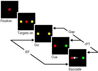
Figure 1. Schematic of the compelled-saccade task. In each trial, the subject must make an eye movement to the peripheral spot that matches the color of the fixation point (red, in this example). Crucially, the disappearance of the fixation point (Go), which instructs the subject to make a saccade, occurs first, before the identities of the target and distracter are revealed (Cue). Task difficulty is controlled by adjusting the time gap between the go and the cue (50–250 ms). In each trial, the reaction time (RT) is the interval between the go signal and saccade onset, and the maximum stimulus viewing time is the raw processing time (rPT), as shown.
Performance in this task can be understood as follows. When the gap is very short (say, zero), the cue is shown early and there is ample time to view the two spots, discriminate target from distracter, and make an informed choice. In contrast, when the gap is very long (say, infinite), the cue is unavailable, and so the subject must guess and make an uninformed, random choice. Thus, task difficulty can be controlled by varying the gap between short values, at which ∼100% correct performance is expected, and long values, at which ∼50% or chance performance is expected. Gap values vary randomly from trial to trial, and so task performance is a mixture of guesses and informed discriminations.
This task design has several interesting features which we discuss below, but there is a basic question that arises often: couldn’t the subjects simply wait for the cue? And if they did, how could we tell, and what would be the consequences? The answers are important because they would strongly constrain the underlying neural mechanisms for generating choices during the task and, in particular, the ways in which perceptual information guides subsequent motor actions.
To investigate these issues, here we construct computational models that simulate performance in the compelled-saccade task based on several possible waiting scenarios, and compare the results with those of an earlier race-to-threshold model (Stanford et al., 2010). Mechanistically, the fundamental difference between the two types of model is whether an oculomotor plan that is already developing can be altered on the fly by the cue information (race model) or not (waiting models), in which case the oculomotor preparation does not change once it has been set in motion. We find that, although it appears intuitive that the subjects performing the compelled-saccade task could simply wait for the cue, in fact, the most natural implementation of such strategy cannot account for the experimental data at all; a good fit can be obtained, but only with a more intricate version of the waiting model which, ultimately, is also inconsistent with experimental evidence. These results narrow considerably the possible neural dynamics of the oculomotor circuits at work during the compelled-saccade task.
2 Materials and Methods
2.1 Behavior and Electrophysiology
The output of the computational models is compared to the behavioral data from two monkeys trained to perform the compelled-saccade task. These benchmark data are the same that were reported previously (Stanford et al., 2010).
All experimental protocols complied with the National Institutes of Health Guide for the Care and Use of Laboratory Animals, USDA regulations, and the policies set forth by the Wake Forest University School of Medicine Animal Care and Use Committee (ACUC). For each monkey, before behavioral training, an MRI-compatible titanium post was attached to the skull under general anesthesia. During subsequent training and data-collection sessions, the post served to restrain the monkey’s head. Eye movements were monitored either with an implanted eye coil (monkeys S), which provided an analog signal of eye position at a rate of 500 Hz, or with an EyeLink1000 (SR Research) infrared tracking device (monkey G) with a sampling rate of 1000 Hz.
Stimuli were colored spots presented through an array of light-emitting diodes (LEDs) placed at a viewing distance of 145 cm from the monkey’s chair. Adjacent LEDs were separated by about 1° or 2° of visual angle. Pairs of saccade targets were placed at various positions and orientations around the central fixation spot, and were separated by 10–20° of visual angle. Gap values varied between 25 and 250 ms. RT was measured as the amount of time from the go signal until the velocity of the saccade reached a cutoff value of 50°/s. To make the appearance of the go signal unpredictable, the delay between the onset of the yellow choice targets and the go was either 500, 750, or 1000 ms, selected randomly in each trial. After the go signal, monkeys had up to 600 ms to initiate a response; responses that took longer caused the trial to be aborted. Correct saccades were rewarded with a drop of water. Red and green targets were presented with equal probability at all target locations.
The neural recording techniques and population of cells chosen for analysis were the same as reported earlier (Stanford et al., 2010).
2.2 Data Analysis
The raw processing time (rPT) is defined as

where the RT and gap values are for a given, individual trial. The rPT is the maximum amount of time that was potentially available for processing the sensory cue in a trial. The effective processing time (ePT) is

where the constant TND is the total non-decision time. In the models discussed here, TND represents the sum of the afferent and efferent delays, averaged across trials, of the circuit that generates a saccadic choice (see below). The tachometric curve is the percentage of correct responses plotted as a function of either rPT or ePT. The choice of rPT or ePT is a matter of convenience: because TND is a constant, the shape of the resulting curve is the same, and the only difference is the value of the origin of the x axis. Here we consider tachometric curves as functions of rPT only, but these are equivalent to those published earlier in terms of ePT (Stanford et al., 2010). Tachometric curves were constructed by calculating the percentage of correct responses for all the trials within an rPT bin, where the bin size was 20 ms and bin centers were spaced every 2 ms.
2.3 Modeling
All model simulations were run in Matlab (The Mathworks). For each model, the free parameters were optimized to minimize the mean absolute error between the simulated and the experimental data for each animal. Thus, for each model, the error function had the form
where e and m are experimental and model values, respectively; the index i = 1,2,…6 identifies each of six psychophysical data sets (or curves) derived from each experiment: psychometric, chronometric (mean and SD) and tachometric curves, and rPT distributions for correct and error trials; the index j runs through each point in a curve; the factor ni is the number of points in curve i; and Ni normalizes the contribution of each curve according to its range of values. So, for instance, if curve 1 consists of 9 points and these vary between 0.6 and 1.0, then n1 = 9 and N1 = 0.4. Best-fitting parameter values were found by exhaustive search.
2.3.1 The accelerated race-to-threshold model
The race model is nearly identical to the one reported earlier (Stanford et al., 2010; see below). It represents the activity of a motor/premotor neural circuit in which sensory information modifies a developing motor plan for generating an impending eye movement. The model consists of two competing variables, xL and xR, that represent the mean activity of neurons that trigger eye movements to the left and to the right, respectively. One race corresponds to one behavioral trial. In each race, both variables start at 0 and the winner is the first one to reach 1000 units. The outcome of the race is taken as a movement to the left if xL wins, or a movement to the right if xR wins.
Each race has two parts, one (before the cue information arrives) during which the build-up rates of xL and xR are constant, and another (after the cue information arrives) during which the build-up rates themselves change at constant rates. The key idea is that, once the cue information becomes available to the circuit, it speeds up the ongoing oculomotor plan toward the target side and slows down the ongoing plan toward the distracter side. Specifically, if the target is on the right side, then xR accelerates and xL decelerates; and vice versa, if the target is on the left, then xL accelerates and xR decelerates.
Each simulated trial proceeds as follows. The go signal occurs at t = 0, and the race starts after an afferent delay TA. The initial build-up rates for xL and xR are drawn from a two-dimensional Gaussian distribution with mean rG (same for both variables), SD σG (same for both variables) and correlation coefficient ρG. When ρG is negative, as was the case for all data fits, the initial build-up rates are anticorrelated. This means that when xL starts increasing at a high rate, xR increases at a much lower rate or may even decrease, and vice versa. During this stage xL and xR change according to
where  and
and  are the initial build-up rates. If one of the variables reaches threshold during this stage, the outcome is a coin toss, because the build-up rates were drawn randomly from a symmetric distribution. Otherwise, xL and xR continue developing as prescribed by the equations above until the cue information reaches the model circuit. This happens at t = gap + TA, because the cue is revealed at t = gap. Once the cue information is available, the two variables start accelerating depending on the locations of the target and distracter. If the target is on the right side, then the build-up rate of xR approaches a large, positive value rT and the build-up rate of xL approaches a small or negative value rD. In this case, the corresponding equations are
where τ is a time constant that determines how long it takes for the rates to reach their new target values. Note that, in the last two equations, the right sides do not change with time; this corresponds to the assumption that the cue-related acceleration is constant. Importantly, however, once the build-up rates reach their new target values, that is, once rL = rD and rR = rT, they stop changing. Thus, rT is the maximum possible build-up rate for the variable that generates a movement toward the target.
Now, if the target is on the left side instead, the roles of xR and xL are reversed: rL approaches rT and rR approaches rD with the same dynamics as before, so
in this case. This integration process continues until xR or xL reaches threshold, and a saccade is assumed to occur a short efferent delay TE after that. The outcome (saccade direction) and RT are then recorded for the trial.
In addition to this basic scheme, there are three important modifications to consider. The third one is implemented slightly differently than in our original report (Stanford et al., 2010), and produces marginally better fits. First, we observed that the monkeys occasionally made mistakes even when they had enough time to make an accurate color discrimination. To account for such errors at long rPTs, in each simulated trial there is a small probability pe of making an incorrect assignment; that is, of associating the target and distracter rates rT and rD with the wrong (i.e., reversed) locations. This amounts to exchanging Eqs. 5 and 6 with a probability pe. Second, the afferent delay is assumed to vary across trials and independently for the go and cue signals. This variability is Gaussian with a SD σA, but such that negative delays are not allowed. Third, the rise to threshold is interrupted between t = I1 and t = I2. During this brief lapse neither xL nor xR (nor their build-up rates) change. This interruption is included to account for a dip that is seen in the rPT distributions of the monkeys; it has a relatively minor effect on the rest of the curves. The onset and offset times I1 and I2 are constant and are given with respect to the point in time when the cue information arrives at the circuit. For example, if I1 = −10 and I2 = 5, the interruption starts 10 ms before the cue information arrives and lasts 15 ms.
The way this interruption was implemented accounted better for the data than other schemes that were tested. However, it may seem puzzling that the interruption can occur before the cue information arrives to the circuit. There are two explanations to this paradox, which are not mutually exclusive. First, the interruption could be effected by other circuits that receive that information earlier than the oculomotor circuit where the race takes place. Second, whereas the cue information that is relevant for the model is specific for color, this is not necessarily the case for the interruption. That is, the interruption may be due to the detection of the cue (“something changed in the sensory environment”) occurring before its content (“red or green”) is determined. This is consistent with the general finding that RTs for detection are generally shorter than for discrimination (Luce, 1986; Sanders, 1998).
In all, the race model has 11 free parameters that were adjusted to match each monkey’s data (Table 1). The model does not distinguish between the afferent and efferent delays; it is only their sum, the total non-decision time, that matters. The total non-decision time varies across trials because it inherits the variability of TA. The single parameter TND represents the mean value of the total non-decision time, averaged across trials. The model produces different outcomes and RTs from one trial to another primarily because different initial build-up rates  are drawn for each trial; the variability of TA, which is the only other independent quantity that also changes in every trial, has a more modest influence on the results.
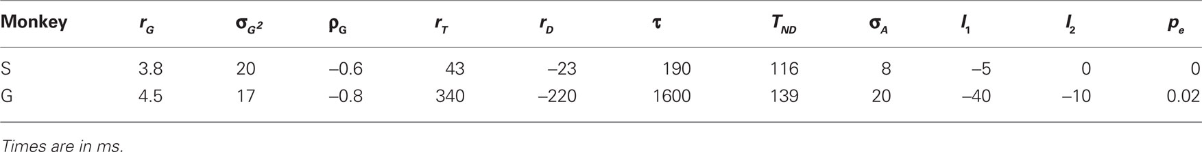
Table 1. Best-fitting parameter values for the race-to-threshold model.
2.3.2 All-or-none waiting
In contrast to the accelerated-race model just described, in which the cue information alters the ongoing oculomotor plan, in the waiting models the subject is assumed to wait until the cue is revealed before starting to prepare an eye movement to indicate his choice. That is, the subject does not initiate a response unless target and distracter have been perceptually disambiguated – so after such waiting the choice is always correct. Importantly, if in a particular trial this idealized subject does not wait, then the direction of the resulting eye movement is random, because the choice was made without any guidance from the cue. The developing oculomotor plan in these models is again represented by a variable (y) that rises toward a threshold, but the plan is always unambiguous, in the sense that it does not change (i.e., accelerate or decelerate) once it has been initiated.
In the Section “Results” we discuss several possible waiting scenarios because performance depends on how exactly the waiting is characterized. One alternative is to ask, in each trial, how likely is it that the subject will wait? This leads to the all-or-none waiting model, which is the most intuitive. In this case there is a probability pW of waiting successfully. If the circuit does wait, target and distracter are located, and a correct, directed saccade is produced, whereas if the circuit does not wait, a random saccade is produced. Another option is to ask, again in each trial, how long can the subject wait? This leads to the stochastic-waiting-model. In this case the subject can wait upto TW ms before initiating the oculomotor plan. If TW is long enough, the cue is seen and a directed saccade is produced, whereas if TW is too short, a random saccade is produced.
In terms of model implementations, the all-or-none version is a special case of the stochastic waiting model, but conceptually they correspond to different cognitive strategies. This is another reason why we present them as separate models. The more general, stochastic waiting model is described in the next section; specific differences between the stochastic and all-or-none waiting models are mentioned at the end.
2.3.3 The stochastic waiting model
In the stochastic waiting model, the subject can wait up to a certain amount of time, but this amount varies randomly across trials. This represents a situation in which the subject tries to wait for the cue but may not be able to control exactly how long. The oculomotor circuit produces either a random saccade to one of the two possible choice locations, or a directed saccade to the target. The first option occurs when the waiting time is too short, and so the eye movement is made without guidance from the cue; the second option occurs when the waiting time is long enough for the target and distracter to be discriminated before the saccadic choice is initiated, and so the resulting eye movement is to the correct location. Different outcomes are produced because the maximum waiting time varies stochastically across trials.
Each simulated trial proceeds as follows. The go signal occurs at t = 0, but it reaches the model circuit after an afferent delay TA. The build-up of activity, however, does not start immediately. Its exact onset time depends on the maximum waiting time TW for the current trial, which is drawn from a unimodal, skewed distribution. Given TW, the latest point in time at which the circuit can start the rise to threshold is trise = TA + TW. On the other hand, the target location becomes known to the circuit at tcue = gap + TA + TD, where TD is the additional time that upstream sensory circuits consume in order to discriminate target from distracter. Therefore, there are two options. First, if trise < tcue, then the wait was not sufficient for the cue information to arrive; a random saccade is produced, with the build-up starting at t = trise. Second, if trise ≥ tcue, then the wait was successful; a directed saccade to the target is produced in this case, with the build-up starting at t = tcue. In each case, once the choice location is determined, the variable y starts increasing linearly, and a saccade is produced TE ms after y reaches a threshold of 1000 arbitrary units.
In each trial, the maximum waiting time TW is drawn from a unimodal but asymmetric distribution composed of two half-Gaussian functions with a common peak (see Hinkle and Connor, 2005). Three model parameters are used to specify this distribution: Tpeak, which is the peak waiting time (i.e., the most common waiting time), σS, which is the SD for waiting times smaller than Tpeak (left side of the distribution), and σL, which is the SD for waiting times longer than Tpeak (right side of the distribution).
In addition, four more parameters are used to described the latencies of random and directed saccades. During random saccades, left and right choices have equal probability, and regardless of saccade direction, the build-up rate for the oculomotor variable y is drawn from a Gaussian distribution with mean μ1 and SD σ1. During directed saccades, the choice is always to the target, and thus always correct, and again regardless of saccade direction, the build-up rate of y is drawn from a Gaussian distribution with mean μ2 and SD σ2. Here, we use the linear rise to threshold with a rate drawn from a Gaussian distribution as a heuristic mechanism for saccade generation; this is because it is a simple process that is known to produce realistic saccadic latency distributions under a wide variety of conditions (Carpenter and Williams, 1995; Reddi and Carpenter, 2000; Brown and Heathcote, 2007).
Finally, there are two important additional components of the stochastic waiting model that are the same as in the race model. First, a separate mechanism is used to account for mistakes that occur when the waiting time is long: in each trial in which a directed saccade is generated, there is a small probability pe of making the saccade to the wrong location. Second, the afferent delay is assumed to vary across trials and independently for the go and cue signals. Therefore, for each signal (in each trial), the afferent delay is equal to a mean plus a variable part that is drawn from a Gaussian distribution with a SD σA.
In all, the stochastic waiting model has 10 free parameters that were adjusted to match each monkey’s data (Table 2). Like the race model, this model does not distinguish between the afferent and efferent delays, so again the single parameter TND represents the mean of their sum. In Table 2, the discrimination time (TD) is also listed as a model parameter, but it is not independent; that is, changing TD is exactly equivalent to changing a combination of other parameters. However, TD is listed separately because it is useful conceptually, and makes one of the hypothetical experiments discussed below easy to implement. The model produces different outcomes across trials primarily because a different maximum waiting time is drawn in each one. In contrast, the variability in RTs depends both on the different TW values and on the variability in the build-up rates (σ1 and σ2). Here again, the variability in the afferent delay also influences outcomes and RTs, but has a modest influence on both.
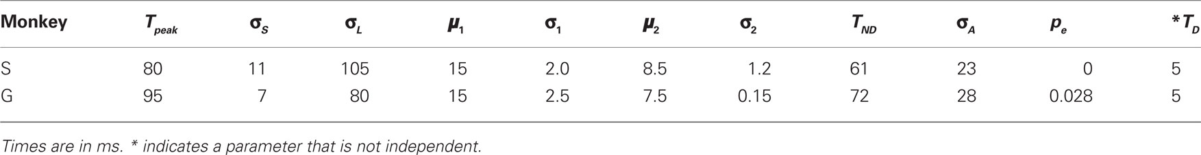
Table 2. Best-fitting parameter values for the stochastic waiting model.
To reproduce the experimental rPT distributions more accurately (particularly in the case of monkey G), the accelerated race model includes two parameters, I1 and I2, that model a short interruption in the development of the saccadic plan. A similar mechanism could have been included in the stochastic waiting model too, but we opted not to do so for the sake of simplicity and to maintain the total number of parameters manageable. Such a mechanism may have produced slightly better fits to the data, as it did in the race model, but this would not have changed any of the conclusions.
In the all-or-none version of the model, the subject simply decides whether to wait or not, and if he does, the wait can be as long as necessary. Therefore, the distribution of maximum waiting times in that case is binary: TW is either infinite (with probability pW) or 0 (with probability 1 − pW). The probability pW replaces the distribution parameters Tpeak, σS, and σL. The saccade-generation mechanisms and the rest of the parameters are exactly as described for the stochastic waiting model.
3 Results
3.1 Psychophysical Performance in the Compelled-Saccade Task
As reported earlier (Stanford et al., 2010), the behavior of two monkeys trained to perform the compelled-saccade task was characterized through five psychophysical curves (Figure 2). First, the psychometric curve plots the percentage of correct responses as a function of the control parameter, the gap (Figure 2A). As expected from the task’s design, performance is close to 100% correct at short gaps, when the cue is revealed shortly after the go signal, and is close to chance, or 50% correct, at long gaps, when the eye movement is often executed before the cue is revealed.
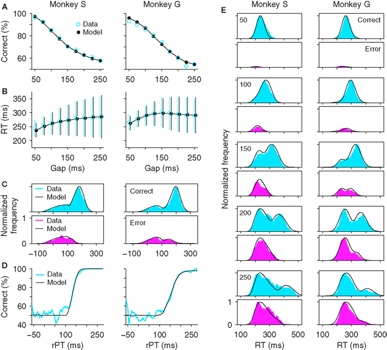
Figure 2. Psychophysical performance of monkeys S and G in the compelled-saccade task. In all panels, experimental data are in blue and magenta, and simulation results from the accelerated race model are in black. For each monkey, the same model parameters were used in all panels (Table 1). (A) Percentage of correct responses as a function of gap (psychometric curve). Each data point includes 568 ≤ n ≤ 598 trials for monkey S and 702 ≤ n ≤ 777 trials for monkey G. (B) Reaction time as a function of gap (chronometric curve). Data points are mean values, which include both correct and incorrect trials at each gap. Error bars indicate ±1 SD. (C) Distributions of rPT values for correct (top) and incorrect (bottom) trials. Bin size is 20 ms. A value of 1 corresponds to the maximum number of observations in correct trials. Data are from a total of 5231 and 6676 trials for monkeys S and G, respectively. (D) Percentage of correct responses as a function of rPT (tachometric curve). (E) Reaction time distributions in correct and incorrect trials at specific gaps. Gap values are indicated on upper left corners. Bin size is 40 ms. Experimental data are as reported earlier (Stanford et al., 2010).
Second, the chronometric curve plots the mean RT ± 1 SD as a function of gap (Figure 2B). This curve is markedly different from what is typically seen in other choice tasks, where RTs may vary several fold as the difficulty of the task changes (e.g., Roitman and Shadlen, 2002; Palmer et al., 2005). Here, it is approximately flat; the mean RT stays relatively constant while performance varies between chance and near perfect.
The third and fourth curves are the distributions of rPT values for correct and error trials (Figure 2C). The rPT is the key quantity that can be extracted in the task; it is the maximum amount of time that the subject has for viewing the cue in any given trial (Eq. 1), so performance is expected to change sharply as a function of rPT. For each monkey, the rPT distribution from error trials overlaps very tightly with the left side of the distribution from correct trials. This is consistent with the idea that the subjects make either fast guesses (∼50% correct) or slower, informed discriminations (∼100% correct) during the task. The range in which the distributions overlap corresponds to the guesses.
Finally, the fifth psychophysical curve shows the percentage of correct responses as a function of rPT (Figure 2D). We call this curve the tachometric curve (Stanford et al., 2010). In judging the tachometric curve, it is useful to keep in mind that negative rPTs correspond to trials in which the eye movement was initiated before the cue was revealed. In these cases the RT is short, smaller than the gap, and so the difference RT − gap (=rPT) is negative. Performance for negative rPTs is expected to be squarely at chance. The slope of the tachometric curve is a direct indication of how much cue exposure time a subject needs in order to perform the task at a particular level above chance. For instance, the curves for monkeys S and G go from chance (50% correct) to 75% correct in only 26 ± 2 and 42 ± 2 ms, respectively (±1 SE; Stanford et al., 2010). This curve, which characterizes the discrimination capacity of a subject, is the key piece of information provided by the compelled-response design.
In the rest of the paper we explore two types of neural mechanisms or circuit dynamics for generating saccadic choices that may explain these experimental data.
3.2 The Accelerated Race Model
The psychophysical curves just described can be replicated quite closely by a simple model in which two variables representing oculomotor activity in favor of rightward and leftward saccades, xR and xL, race to a threshold (Stanford et al., 2010; Figure 2, black traces). In each trial, the winner determines the direction of the resulting eye movement, and the RT is equal to the time taken to reach threshold. A detailed description of the model and its parameters is given in the Section “Materials and Methods,” but in essence, the model has two main features: (1) once the go signal reaches the model circuit, which depends on an afferent delay, the two variables start increasing with initial build-up rates that vary randomly from one trial to another, and (2) once the cue information reaches the model circuit, after the gap has elapsed, the variable representing the oculomotor plan toward the target accelerates, and the variable representing the plan toward the distracter decelerates. Thus, depending on the initial build-up rates and on the gap in each particular trial (Figure 3A), the model can produce either informed discriminations (Figure 3B) or fast guesses (Figure 3C). For the purpose of contrasting this model with the waiting models discussed below, the key here is that the oculomotor plans are set in motion immediately after the go signal is received – without waiting – and that the arrival of the cue information modulates the build-up rates of those plans while they are ongoing; the saccadic choice is adjusted on the fly.
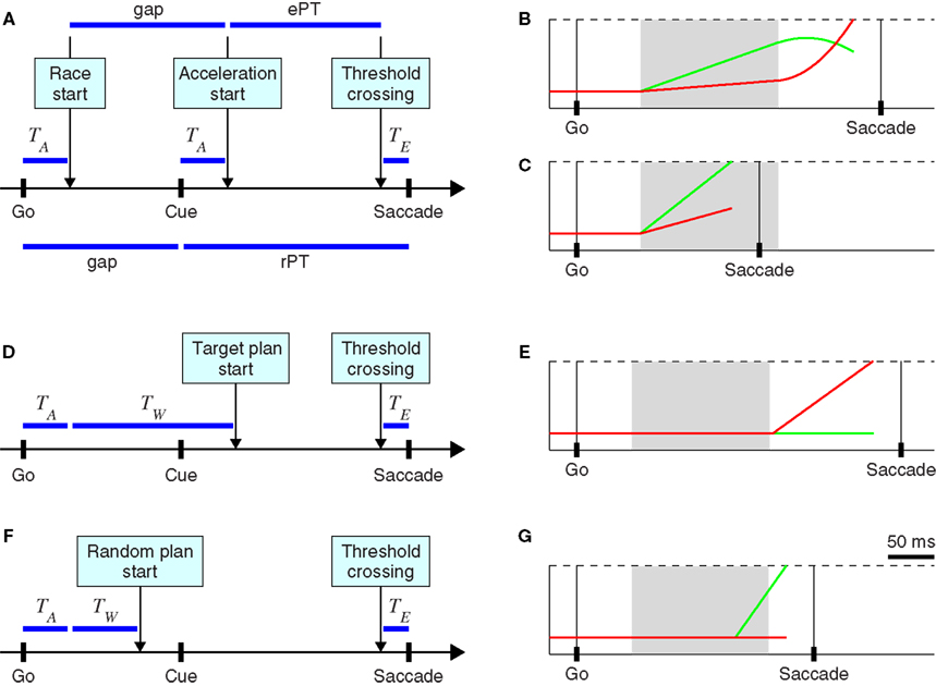
Figure 3. Two types of models for generating oculomotor choices in the compelled-saccade task. (A) Schematic of the accelerated race-to-threshold model. The arrow shows the timeline of the three key events in each trial (Go, Cue, and Saccade). The boxes above indicate events that occur within the oculomotor circuit, and their timing. TA and TE indicate afferent and efferent delays, respectively. (B) A trial of the accelerated race model in which the cue information arrives in time to alter the ongoing oculomotor plans, producing a correct response. Red and green traces correspond to neural responses favoring rightward and leftward saccades, respectively. The cue information becomes available at the end of the gray shade, when the acceleration starts. (C) A trial of the accelerated race model in which a saccade is triggered before the cue information arrives, resulting in a wrong guess. (D) Schematic of the stochastic waiting model when the waiting time TW is long, and so the saccadic response is toward the known target location. (E) Model neuronal activity in one trial of the type schematized in (D). (F) Schematic of the stochastic waiting model when the waiting time TW is short, and so the saccadic response is random. (G) Model neuronal activity in one trial of the type schematized in (F). In all examples, the target is assumed to be located to the right of fixation, so trials in which the red trace (xR) crosses threshold (dotted lines) first are correct and trials in which the green trace (xL) crosses threshold first are errors.
The accelerated race-to-threshold model not only fits the five psychophysical curves discussed in the previous section, but also predicts the shapes of the RT distributions for error and correct trials obtained for each individual gap (Figure 2E). These distributions change quite dramatically: at short gaps most responses are fast (RT < 300–350 ms) and correct, whereas at long gaps the fast responses are about equally likely to be correct or incorrect, but there are also many slow responses (RT > 300–350 ms), most of which are correct. At intermediate gaps there is a transition between these two regimes, such that the RT distributions for correct trials are bimodal. This progression is accurately captured by the accelerated race model.
The question, however, is whether the experimental data could also result from a rather different oculomotor choice process.
3.3 Three Ways to Wait
The bimodal RT distributions just discussed, and their progression, are consistent with the idea that there are two types of trials in the task, guesses, and informed discriminations. In the race model, whether a particular trial results in a guess or an informed choice depends on the initial build-up rates drawn in that trial, and on the gap; the dynamics of the model circuit then determines the outcome. But intuitively, the subject’s choice in each trial could instead depend on whether he or she waits for the cue or not. In other words, after seeing the go signal (offset of the fixation spot) the subject could withhold the response, wait for the target and distracter to be identified, and then initiate an eye movement to the target (Figures 3D,E).
In this situation, the observed behavior will depend critically on how exactly the subject waits, or what exactly is meant by waiting. For instance, the subject may wait until the cue is seen in some trials only, but not in all of them; or perhaps the wait always occurs but is long enough only in a subset of the trials (Figures 3D–G). These distinctions are subtle but make a large difference in the psychophysical responses that are produced, as shown below. To explore these scenarios quantitatively, we considered three possible waiting strategies and generated corresponding model circuits that simulated performance in the compelled-saccade task.
3.3.1 All-or-none waiting
In the situation that is perhaps most intuitive, the subject simply waits for the cue to be revealed and makes an informed saccadic response. If the subject can always wait for the color discrimination to be over before starting the saccadic choice process, then, regardless of how long the wait needs to be, the choice is always (or nearly always) correct. Precisely for this reason, however, this strategy can be readily ruled out: it predicts that the percentage of correct responses should be close to 100% for all gaps, and this is clearly not the case (Figure 2A). Therefore, for sure the monkeys do not always wait.
A more nuanced version of this strategy is one in which the subject waits for the cue in some trials but not in others. To simulate this case, we made two assumptions: (1) that the probability that the subject waits in any trial is pW, and (2) that the oculomotor plans are not modified once they are initiated. Thus, in trials in which there is no waiting, the response is an eye movement to one of the two locations chosen randomly, and in waiting trials the response is an eye movement to the target. We call this the all-or-none waiting model (see Materials and Methods). The motor plans for random saccades (no wait) are initiated right away, after the go signal reaches the model circuit, whereas the motor plans for directed saccades (yes wait) are triggered shortly after the cue information reaches the model circuit, under the assumption that the actual color discrimination takes an additional, fixed amount of time (TD). In either case, the motor plans never accelerate or change otherwise once the build-up has started (see Materials and Methods for details). The choice in this model is very simple: to wait or not to wait.
This all-or-none waiting strategy, however, still fails to reproduce the basic psychophysical results that are characteristic of the task (Figure 4). First and foremost, the percentage of correct responses for this model is the same at all gaps (Figure 4A). This is because the probability of waiting in any given trial is constant, and is therefore independent of the gap (recall that, during the experimental sessions, gap values were chosen randomly in each trial; for this reason, in all the models they were assumed to be unpredictable). Different values of pW shift the psychometric function up or down because pW directly determines the success rate, but the resulting curve is always flat, regardless of the dynamics of the saccadic responses. Second, waiting trials at longer gaps produce correspondingly longer waits, so the mean RT always increases linearly as a function of gap (Figure 4B). The slope of this linear relationship may vary depending on model parameters, but a linear increase is always present.
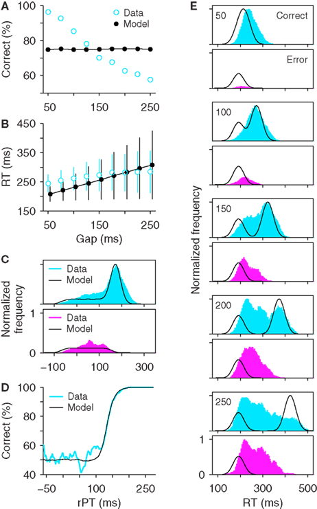
Figure 4. An all-or-none waiting model cannot reproduce the experimental data. In each trial of the model the subject waits for the cue with a probability pW. If he does wait, a correct saccade to the target is produced; otherwise, a random saccade, or guess is produced. Thus, waiting times are either 0 (no wait) or equal to the gap plus a constant (yes wait). Experimental data from monkey S are in blue and magenta; best-fitting simulation results are in black. (A) Psychometric curves. The all-or-none model produces the same percentage of correct responses at all gaps. (B) Chronometric curves. The model’s mean RT increases linearly with the gap. (C) Distributions of rPT values. (D) Tachometric curves. (E) Distributions of RTs at specific gaps. Note that the model distributions consist of stereotypical curves that do not vary in width or height as the gap changes.
In spite of these problems, this model is instructive because it can indeed produce rPT distributions that reflect two different processes, fast guesses, and slower, informed discriminations (Figure 4C). Also, although the shapes of these distributions certainly differ from those obtained experimentally, the model can produce tachometric curves that match the experimental data extremely well (Figure 4D). The model’s mixtures of random and directed saccades again differ quite obviously from the experimental data when the distributions of RTs for correct and error trials are plotted for specific gaps (Figure 4E). In the RT distributions obtained from the model, the only feature that varies across gaps is the position of the second peak in correct trials; the other peaks remain constant. This problem is directly related to the flat psychometric curve: the proportions of random and directed saccades are constant, and the only quantity that can change systematically across gaps is how long the directed saccades take.
3.3.2 Waiting to accelerate: a hybrid model
The two assumptions of the all-or-none model are that the subject waits with a probability pW, and that once a motor plan is initiated, it cannot be modified by the sensory information. The second assumption may seem too drastic; one may wonder what happens if, for instance, the subject is able to wait a limited amount of time but the motor plan can still be modified on the fly in case the wait is not long enough to identify target and distracter. The consequence of waiting in this case turns out to be quite mild, in the sense that once the ramping at different rates can be altered by incoming sensory information, the evolution of the perceptual discrimination can be accurately captured by the tachometric curve and the dynamics of the accelerated race, whether or not there is an additional delay due to the waiting. This suggests that the serial arrangement between the sensory and motor processes in the all-or-none waiting model is the fundamental feature that differentiates it from the accelerated race model.
To explore this hybrid scenario, we investigated how waiting would impact the performance of the accelerated race-to-threshold model. In this case, waiting is understood simply as an extra delay: the subject does not start his or her motor preparation immediately once the go signal is seen – there is an additional waiting time TW – but once the cue information arrives at the circuit, the acceleration proceeds exactly as before. That is, the variables xL and xR start building up later than usual, up to TA + TW ms after the go signal is given, where TA is the afferent delay, but once the cue information becomes available to the circuit, the acceleration process begins whether the waiting time has fully elapsed or not. In this way, the waiting time effectively shortens or may even eliminate the initial build-up of activity in the model, during which the build-up rates are random, but does not change the dynamics of the cue-driven acceleration.
Figure 5 compares the performance of the race-to-threshold model with (right column) and without (left column) waiting. The simulations proceeded in the same way in the two cases, as explained above, except for the maximum waiting time TW, which was drawn from an exponential distribution in each trial of the hybrid model (Figure 5, caption). In general, waiting increased the overall performance level and the mean RT in the task (Figures 5A,B), as one might have expected intuitively, but it did not affect the tachometric curve at all (Figure 5D). Identical tachometric curves were also obtained with a variety of waiting time distributions that were tested, so the results were the same regardless of the shape of the waiting time distribution.
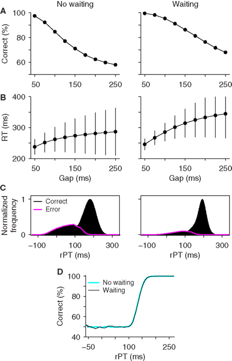
Figure 5. Effect of waiting within the accelerated race-to-threshold model. The accelerated race model was simulated under standard conditions (no waiting) and with maximum waiting times drawn from an exponential distribution with a mean of 75 ms. Parameters were as listed in Table 1 for monkey S. (A) Psychometric curves. (B) Chronometric curves. (C) Distributions of rPT values in correct (black) and error (magenta) trials. (D) Tachometric curves. Although waiting generally alters the observed task performance, it does not affect the tachometric curve.
The reason for this is that waiting does not affect the acceleration process, which is primarily what determines the tachometric curve and what relates to perceptual processing speed in the race model. Waiting does alter how long the cue-driven acceleration lasts, but this is precisely what is quantified by the processing time rPT, i.e., the maximum stimulus viewing time in each trial, and rPT is still accurately calculated as the difference RT − gap (Equation 1) regardless of the waiting time. Therefore, the tachometric curve still isolates the subject’s perceptual performance. This type of waiting may change some of the psychophysical curves quantitatively, but is otherwise of little consequence for interpreting the model’s results (see also the Supplementary information in Stanford et al., 2010).
In conclusion, if understood as a simple delay to respond, waiting can be easily incorporated within the accelerated race model. This includes the possibility of very long waits on just a fraction of the trials, or other possible waiting time distributions. However, as long as the cue-driven acceleration mechanism stays in place, waiting is of relatively little consequence because it does not distort the measured rPTs nor the tachometric curve. Thus, waiting, if it happens at all, does not affect the interpretation of the results and is essentially harmless within the dynamical framework of the race model. Now, with respect to the actual experimental data, the match between model and experiment in Figure 2 suggests that, if the accelerated race model is correct, then the monkeys did not delay their responses once the go signal had been detected, because the model used in Figure 2 did not include any waiting.
This is not to say that waiting, as implemented in the hybrid model, could never occur; dramatic changes in RT and performance levels can be generated during the task by differentially rewarding the possible outcomes, so subjects can slow down and speed up their responses according to the task’s contingencies (see motor bias experiment in Stanford et al., 2010). Although these reward-dependent biases have been accounted for by the accelerated race model, substantial behavioral flexibility suggests that an effect like that in Figure 5 might be possible given the appropriate experimental circumstance. Crucially, though, this would not be diagnostic of a mechanism fundamentally different from the accelerated race, and would not alter the interpretation of the results in a significant way.
3.3.3 The stochastic-waiting model
We now consider one last waiting scenario in which, as in the all-or-none model, we assume that once a motor plan starts developing, it is not modified by incoming sensory information. The idea is to remedy the flaws of the all-or-none waiting model by considering a similar but somewhat more sophisticated waiting strategy, which is as follows.
Suppose that the subject tries to wait for the cue but cannot fully control how long. So, in any given trial, there is a maximum amount of time that the subject can wait, but this amount varies randomly and unpredictably. In each simulated trial, a maximum waiting time TW is drawn from a distribution, and when the go signal reaches the circuit, the saccadic motor plan is withheld. If the target and distracter identities become known to the circuit before TW has elapsed, then a directed saccade to the target is prepared; otherwise, if the waiting time expires before these identities are revealed to the circuit, then a random saccade to one of the two locations is prepared. Because TW is sampled from a distribution, we call this the stochastic waiting model.
In all the models considered in this article, with and without waiting, the preparation to make a saccade corresponds to the build-up of neuronal activity toward a threshold, and the saccade is assumed to be triggered once that threshold is reached (the actual saccade onset is considered to occur TE ms after threshold crossing, where TE is the efferent delay). Neurophysiological (Hanes and Schall, 1996; Roitman and Shadlen, 2002), psychophysical (Carpenter and Williams, 1995; Reddi and Carpenter, 2000; Brown and Heathcote, 2007) and modeling (Lo and Wang, 2006) data indicate that this is a reasonable simplification of the actual process. In the accelerated race model (with and without waiting) the build-up rates can change during the rise, but in the stochastic-waiting model, as in the all-or-none waiting model, those rates cannot change once the build-up has started (see Materials and Methods for details). Another way to state this is that in the accelerated race model the oculomotor plans may be prepared while the outcome (i.e., saccade direction) is still uncertain, whereas in these two waiting models the oculomotor plans are entirely certain from the beginning.
The diversity of maximum waiting times that can be used gives the stochastic waiting model much more flexibility than the all-or-none version. In fact, Figure 6 shows that, if the distribution of maximum waiting times has the correct shape, the model can accurately replicate all the psychophysical data in the task (Figures 6A–D) and can produce RT distributions at individual gaps that are quite close to the experimental ones (Figure 6E). For these simulations, the distributions of maximum waiting times had a single peak and tails of different lengths on the two sides. Three parameters were necessary to describe such distributions (Materials and Methods). Crucially, in this model, the percentage of correct responses changes as a function of the gap, even though the repertoire of maximum waiting times is the same across gaps. What happens is that, at short gaps, the majority of the TW samples are longer than the gap, and so most trials are successful waits that end with a directed saccade to the target (∼100% correct); in contrast, at long gaps, the majority of the TW samples are shorter than the gap, and so most trials are unsuccessful waits that end with a random saccade (∼50% correct).
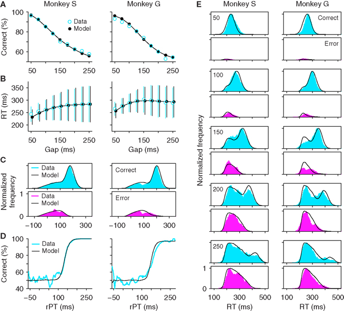
Figure 6. The stochastic waiting model reproduces the psychophysical performance of monkeys S and G in the compelled-saccade task. (A) Psychometric curve. (B) Chronometric curve. (C) Distributions of rPT values for correct (top) and incorrect (bottom) trials. (D) Tachometric curve. (E) Reaction time distributions in correct and incorrect trials at specific gaps. Same experimental data and format as in Figure 2, but with simulation results from the stochastic waiting model. The maximum waiting time TW was drawn from a broad distribution in each trial. This waiting strategy produced good fits to the experimental data.
In Figure 6, the quality of the fits is excellent for monkey S but slightly less so for monkey G. In particular, the model fails to capture the small but appreciable dip in the rPT distributions of both correct and error trials (Figure 6C, monkey G, near rPT = 100 ms), and the model tachometric curve is slightly steeper than the experimental curve (Figure 6D, monkey G). These minor discrepancies could be ameliorated in two ways. First, the dip could likely be replicated by specifying a short interval during which the ramping toward threshold is momentarily interrupted, as done in the race model (see Materials and Methods). And second, the tachometric curve could probably be better matched by considering waiting time distributions with more flexible shapes (e.g., that could have either one or two peaks). However, these modifications would require more parameters. Instead, rather than increasing the complexity of the model, we take Figure 6 as sufficient proof that a waiting strategy can, in principle, explain the psychophysical data in the compelled-saccade task, and therefore, that just by analyzing the behavioral data presented so far, the possibility that the monkeys wait for the cue cannot be ruled out.
So, two distinct neural mechanisms can explain the psychophysical data, cue-driven acceleration and stochastic waiting. In the two remaining sections we explore behavioral and neurophysiological predictions that can distinguish them unambiguously.
3.4 Psychophysical Predictions
To differentiate the accelerated race model from the stochastic waiting model, we consider two hypothetical experiments that are variants of the standard compelled-saccade task. Besides their predictive value, these simulations provide a better intuition of the key differences between the two models.
First, suppose that the difficulty of the sensory discrimination is increased. This can be achieved, for instance, by decreasing the chromatic contrast between the red and green spots, or by having the subject discriminate two similar shapes instead of two colors. The idea is that difficult discriminations should require longer viewing times than easy discriminations for any given percentage of correct responses (Bodelón et al., 2007). If this assumption is correct and all other aspects of the task remain constant, then a clear prediction can be made in each model (Figures 7A,C).
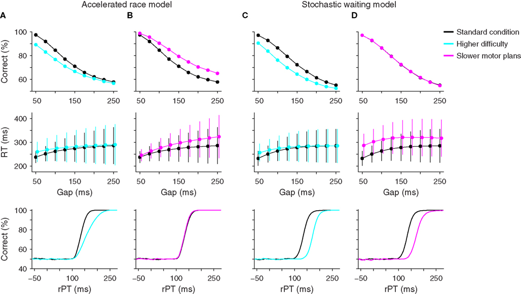
Figure 7. Psychophysical predictions of two computational models. Each column shows psychometric, chronometric, and tachometric curves from two sets of simulations, a standard condition (black points and lines) which uses the parameters that best fit the data from monkey S for each model, and a hypothetical experimental condition. (A) Predicted effects of task difficulty on performance according to the accelerated race model. Increased difficulty in discrimination (blue) was simulated by increasing the acceleration time constant τ from 190 to 437 ms. (B) Predicted effects of motor response time on performance according to the accelerated race model. Slower oculomotor activity (magenta) was simulated by reducing the mean build-up rate rG from 3.8 to 2.5. (C) Predicted effects of task difficulty on performance according to the stochastic waiting model. Increased difficulty in discrimination (blue) was simulated by increasing the sensory discrimination time TD from 5 to 40 ms. (D) Predicted effects of motor response time on performance according to the stochastic waiting model. Slower oculomotor activity (magenta) was simulated by reducing the rates μ1 and μ2 from 15 and 8.5 to 10.5 and 6, respectively. These parameters are the mean rates at which oculomotor activity increases from baseline to threshold when a random location is chosen (μ1) and when the target location is known (μ2). Note the different predictions that the two models make on the psychometric and tachometric curves.
According to the accelerated race model, higher perceptual difficulty should translate into a decrease in the percentage of correct responses and a slight increase in mean RT, particularly at short gaps, but most importantly, it should also produce a shallower tachometric curve (Figure 7A). This is because, in the race model, the slope of the tachometric curve is directly related to the speed of the perceptual process, and a difficult discrimination should require more viewing time than an easy one (Bodelón et al., 2007). To appreciate the generality of this result, consider how the color discrimination enters into the race model. Perceptual performance depends on the strength of the sensory signal, through parameters rT and rD, and on how fast that sensory signal is delivered to the circuit generating the saccadic choice, through parameter τ. But the first two terms appear in the dynamical equations as rT/τ and rD/τ (Eqs. 4–6), so it is these two combinations of parameters that matter the most. They control the cue-dependent acceleration and deceleration of the motor plans, which in turn determine the slope of the tachometric curve. Therefore, variations in task difficulty can be modeled by modifying these two quantities, thus producing tachometric curves with different slopes.
In contrast, although similar effects are expected for the psychometric and chronometric curves according to the stochastic waiting model, its prediction is very different for the tachometric curve: it should shift to the right, without any change in slope (Figure 7C). The reason for this is that, in this model, the slope of the tachometric curve depends principally on the variability of the afferent delay (σA), which is unlikely to be related to task difficulty. Changes to the parameter that corresponds to the sensory discrimination time TD can only shift the curve, and changes to other parameters leave the curve unchanged. Therefore the dependency of the tachometric curve on task difficulty is a robust criterion for distinguishing the two models.
The second hypothetical experiment is complementary to the first. The idea now is to keep the perceptual component of the task constant and manipulate the motor component instead. Specifically, we consider a hypothetical condition in which oculomotor preparation is slower than in the standard compelled-saccade task. Although the hypothetical outcomes are clear, in practice, influencing motor preparation independently of the sensory evaluation is more difficult, but might be accomplished in a variant of the task that places greater demands on the motor choice associated with a particular perceptual discrimination (e.g., Sato et al., 2001).
In the race model such manipulation was assumed to decrease the build-up rates of the oculomotor plans (i.e., rG), effectively slowing down motor execution. This change in parameters caused an increase in both the percentage of correct responses and the mean RT, particularly at long gaps, but it did not alter the tachometric curve at all (Figure 7B). Again, this is consistent with the framework of the model, in which the slope of the tachometric curve is not influenced by motor contingencies and its location along the x axis depends exclusively on the afferent and efferent delays. Also, performance increased because slower movements provide more viewing time, and thus more time for the circuit to accelerate and choose the correct location. Note that, although the tachometric curve did not change, an increase in overall performance resulted because more trials with long rPTs were produced, so more points were sampled from the right side of the curve than in the control case.
In contrast, the stochastic waiting model again predicted a shift of the tachometric curve and an overall increase in RT, but most notably, no change in performance as a function of gap (Figure 7D). Performance did not change because saccades in this model are always made to a location that is certain; the speed of the motor plan has no bearing on the location of the resulting eye movement.
3.5 Neurophysiological Predictions
Another way to distinguish the two candidate mechanisms at hand is to compare the neural activity patterns that they predict with actual neuronal activity recorded directly from oculomotor structures engaged during the task. To generate such predictions, several thousand trials were run for each model, and the simulated motor plans were saved for all trials. Then we computed the average traces of the motor plans in the neurons’ preferred direction and of the plans in the opposite direction. These average traces were calculated with all trials synchronized either on the go signal, on the cue, or on the saccade. In addition, because the rPT is a crucial variable in the task, separate averages were generated for trials with long and with short rPTs (Figure 8). All of these procedures were meant to mimic the standard methods used for analyzing extracellular recordings from oculomotor cells (Thompson et al., 1996; Port and Wurtz, 2009; Stanford et al., 2010).
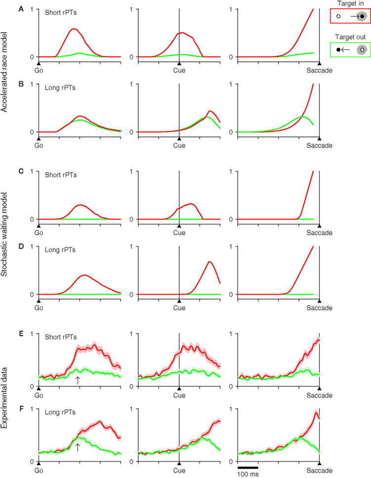
Figure 8. Neurophysiological predictions of two computational models and comparison with experimental data. For each model, 8000 trials were simulated using the parameter values that best fitted the data from monkey S (Tables 1,2). Trials were sorted into two groups, one with short (rPT ≤ 115 ms), and another with long (rPT ≥ 145 ms) processing times. The model responses in each group were aligned either on the go signal (left column), on the cue (middle column), or on the saccade (right column), and were then averaged. Separate averages were calculated for responses in the preferred direction of the model neurons (red traces) and in the antipreferred direction (green traces). Only correct trials were considered. (A) Average neural activity predicted by the accelerated race model in short-rPT trials. (B) Average neural activity predicted by the accelerated race model in long-rPT trials. (C) Average neural activity predicted by the stochastic waiting model in short-rPT trials. (D) Average neural activity predicted by the stochastic waiting model in long-rPT trials. (E,F) Average normalized activity obtained from a population of 30 FEF neurons. Trials were sorted and aligned exactly as described above for the simulated data. Shaded areas indicate ±1 SE across neurons. In all plots, the y axis corresponds to normalized firing rate.
An important consideration here is that the accelerated race model makes specific predictions both for the motor plan in the preferred direction of the neurons and for the plan in the opposite direction, because it is based on two competing populations (Figures 8A,B); whereas the stochastic waiting model only specifies the motor plan in the preferred direction, because there is no explicit competition, only a single motor plan per trial. Although these are shown as flat (Figures 8C,D, green traces), the waiting model simply does not say anything about the motor plans in the antipreferred direction, except that they do not reach threshold.
In spite of this caveat, differences between the two sets of model predictions are easy to appreciate. Notably, the race model generally predicts a larger and earlier separation between the two activity traces on short rPTs than on long rPTs (compare Figures 8A,B). We interpret this phenomenon as follows: when, at the beginning of a trial, it so happens that one of the motor plans builds up much faster than the other, the outcome is typically a fast guess, which results in a short rPT; in contrast, when the two initial build-up rates are moderate, there is more time for the cue signal to accelerate the plan associated with the target, typically producing a correct discrimination with a long rPT. A consequence of this is that the activity in favor of the distracter side (green traces) is generally stronger at long rPTs than at short ones. Thus, in the race model, the competing motor plans not only separate less at long rPTs than at short ones, but also separate much later, on average.
The stochastic waiting model does not specify the motor plan away from the chosen direction, as mentioned above. However, it is possible to compare the activity associated with the winning motor plan (red traces) in short- versus long-rPT conditions. In this case, there are two predictions that are very different for the two models. First, when the data are aligned on the go signal, the race model predicts a higher build-up rate for short than for long rPTs (Figures 8A,B, left column), whereas the waiting model predicts no difference (Figures 8C,D, left column). And second, when the data are aligned on saccade onset, the average rise to threshold is obviously different for the two models: the race model predicts that the average trajectory toward threshold should be steeper and more curved in long-rPT trials than in short-rPT trials (Figures 8A,B, right column), whereas the waiting model essentially predicts the opposite, that a steeper trajectory should be observed in short-rPT trials (Figures 8C,D, right column).
A point to keep in mind about both sets of predictions is that the models do not specify anything after saccade onset. This is important for interpreting the model results aligned on the go or the cue. It means that the predicted average traces apply mainly during the rising phases of the red curves, which mostly reflect the activity leading to saccade onset. In each case, the decrease that follows the peak (Figures 8A–D, red curves in left and middle columns) occurs because progressively fewer trials contribute to the average traces as time increases; that is, trials that end quickly (with short RTs) contribute only to the first part of a trace when the data are aligned on the go or the cue.
These predictions were compared with experimental data recorded from the frontal eye field (FEF). For the comparison, we used a set of 30 FEF neurons with saccade-related activity that were described in an earlier publication (Stanford et al., 2010; neurophysiological methods detailed there). The same population responses were aligned on the saccade, as was done before, and were also replotted synchronized on the go signal and on cue onset (Figures 8E,F). In each case, the activities associated with eye movements into (red traces) and away from (green traces) the movement field showed a close agreement with the average traces predicted by the accelerated race-to-threshold model.
First, consider the data aligned on the go signal (Figures 8E,F, left column). Note what happens at the time point marked by an arrow, 190 ms after the go, at which point the red traces in the two models are either still rising a little or have just stopped (see Figures 8A–D, left column). At this time, the red and green experimental traces are nearly fully separated in short-rPT trials, whereas in long-rPT trials they still have not diverged; this is both because the activity associated with the distracter is higher and because the activity associated with the target is lower than in short-rPT trials. These differences are not seen in the stochastic waiting model, but are very much as predicted by the race model.
Second, consider the experimental data aligned on cue onset (Figures 8E,F, middle column). In short-rPT trials the red and green traces have already diverged substantially by the time that the cue is revealed, whereas in long-rPT trials both traces have just started rising, and do so together for another 110 ms approximately. Again, this is very much as expected from the race model. In contrast, the stochastic waiting model predicts that, during long-rPT trials, activity should start rising about 40 ms after the cue presentation, which is clearly not what happens in FEF.
Finally, consider the experimental data synchronized on the onset of the saccade (Figures 8E,F, right column). As noted in our earlier report (Stanford et al., 2010), there are two important differences between long- and short-rPT trials in this case. First, the neural activity associated with eye movements away from the receptive field (green traces) is stronger in the latter condition, but declines sharply before the saccade is initiated. And second, the neural activity associated with eye movements into the receptive field (red traces) has slightly but significantly different curvature in short- versus long-rPT trials, the latter condition producing a steeper rise in activity. Both effects are in agreement with the results of the race model, and the second one is at variance with what is expected from the stochastic waiting model.
4 Discussion
The compelled-saccade task is useful because it provides, through the tachometric curve, a direct characterization of a subject’s perceptual judgment as it evolves in time; i.e., it shows how long it takes for the subject to make a discrimination regardless of motor execution. With this curve at hand, it also becomes possible to correlate the temporal evolution of the subject’s percept with the temporal profile of activity of a population of recorded neurons, which, in turn, serves to identify their functional impact during task performance (Stanford et al., 2010).
However, a simple but important assumption must be true for this scheme to work: the measured sensory processing time rPT must be proportional to the effective stimulus viewing time, and this exposure time should indeed be the relevant variable determining perceptual performance in the task. This condition is true in the accelerated race model with and without waiting, but it is not satisfied in the stochastic waiting model. Although it produces good fits to the experimental data, including the tachometric curves, in the stochastic waiting model the sensory discrimination time TD is fixed, and the rPT values measured across trials are not causally related to the trials’ outcomes. We found that both models could fit the psychophysical data from the standard compelled-saccade task, but they made mutually exclusive predictions for the behaviors that should be expected under additional task conditions, and for the neural activity that should be observed during task performance.
The present modeling results are interesting because they illustrate how sets of psychophysical data can be simultaneously consistent with drastically different underlying neural mechanisms, even when the experimental curves contain non-trivial features (e.g., two peaks). In addition, they answer several important questions about the compelled-saccade task and the mechanisms for oculomotor choice that may be at work during its execution.
4.1 Did the Subjects Wait for the Cue?
For several reasons, we believe the answer is, no. In its simplest, most intuitive form, a waiting strategy implies a serial process requiring the subject to wait until the perceptual decision is completed before planning a saccade to the chosen target. This all-or-none strategy, which corresponds most closely with the voluntary act of waiting, failed to explain numerous prominent features of the data. Whether applied on every trial or on some fraction of the trials, such an all-or-none waiting regime, in which the subject “waits out” the gap, is clearly inconsistent with the psychophysical data. Most tellingly, it predicts a flat psychometric function (Figure 4A), and a linear rise in the chronometric curve (Figure 4B). Instead, we observed monotonically declining psychometric curves and relatively flat chronometric functions, each readily explained within the framework of an accelerated race model lacking any provision for waiting.
Although waiting in its most deliberate form (i.e., wait until sure, then look) is easily ruled out, the fits to the data obtained with the stochastic waiting model show that it is not possible to rule out a more sophisticated waiting scheme solely on the basis of the current psychophysical findings. Nevertheless, we note that a number of specific conditions must be met for such a waiting regime to work. First, the waiting time cannot exceed the gap on every trial (successful waits), because then performance would be near perfect, and that was not observed. Also, waiting can work, but only if the subject generates waiting times across trials with precisely the correct distribution, and ensuing motor plans develop rapidly enough so that saccades conform to the observed RT distributions.
Although the accelerated race model and the stochastic waiting model both produce good fits to the behavioral data, they imply very different underlying neurophysiological mechanisms (Figure 8). In fact, these two models make opposing predictions for how sensory processing time is manifest in the temporal profile of oculomotor activity. In a recent report, we demonstrated that the motor-related discharge of neurons in the FEF is highly consistent with the temporal interaction between sensory and motor processes predicted by the accelerated race model during performance of the compelled-saccade task (Stanford et al., 2010). Here, we extended those observations by replotting the same experimental data in other ways, namely, synchronized on the go signal and cue onset, thus exposing several characteristic features of the neural activity that can be readily compared against the models’ predictions. The results are clear: in all cases, the FEF responses are inconsistent with those expected from the stochastic waiting model, but match quite closely the results of the accelerated race model.
Beyond the neurophysiological evidence, the two models make distinct predictions for how the degree of perceptual difficulty impacts the psychometric, chronometric, and tachometric curves (Figure 7), and manipulating task difficulty is the basis for planned experiments designed to further distinguish between these alternatives.
4.2 Why didn’t the Subjects Wait for the Cue?
If it is true that our monkey subjects did not wait to see the cue during task performance, one may wonder why not. We think there are at least three reasons.
First, it might simply be very difficult to withhold a saccade when the fixation spot disappears. In fact, the compelled-saccade task is an elaboration of the so-called “gap task,” in which extremely short saccadic RTs to a single target are induced simply by eliminating the fixation spot slightly before target presentation (Saslow, 1967; Paré and Munoz, 1996). It seems plausible that the release from an active state of fixation in conjunction with the presence of two highly salient spots, and a 50% probability of being rewarded for either choice, is sufficient to “compel” the subject to engage saccade planning mechanisms. Put another way, it may be much more difficult to wait, i.e., to stare at the blank screen between the two bright targets, than it is to look at one of them. It is also relevant to note that gap values were randomized, further increasing the difficulty of implementing a purposeful waiting strategy – on any given trial, the subjects do not know how long to wait, if that is indeed what they try to do.
Second, before performing the compelled-saccade task, the monkeys were trained on a traditional choice paradigm that is very similar to the compelled task, except that the cue is revealed before the go signal; this is the easy choice task (see Supplementary information in Stanford et al., 2010). Thus, during training, our subjects learned the rule “move your eyes as soon as the fixation spot disappears.” It is likely that they applied this exact same rule in the compelled version of the task, since transition from the easy to compelled versions required no additional training, and the two task types could be interleaved without any disruption in performance. Logically, the two tasks can be viewed as a continuum, with easy trials having negative gap values, compelled trials having positive gap values, and the transition between the two corresponding to zero gap. Accordingly, RTs in the easy choice task were most similar to those for the shortest gaps in the compelled condition.
Third, although waiting may seem advantageous from the point of view of this particular task, in general, the oculomotor system is not engineered to stop and wait until certain sensory events occur in the world. Normally, primates make about three saccades per second – they do so even in the dark – and the saccade statistics change very little across visual scenes and behavioral contexts (Castelhano et al., 2009). It is only under exceptional circumstances, such as overtrained laboratory tasks, that they fixate for extended periods of time. Four types of experimental observation support the basic premise of the accelerated race-to-threshold model that sensory information guides or modulates oculomotor plans that are already ongoing. (1) In choice tasks in which potential targets are separated by less than 180°, short-latency saccades frequently demonstrate curved trajectories, suggesting that the initial erroneous choices are modified to accommodate new information about the actual target location (McPeek et al., 2003; Walton et al., 2005; McPeek, 2006). (2) While a saccade to a fully known, unambiguous target location is being programmed, the sudden appearance of a distracter can still evoke oculomotor activity and give rise to distracter-directed errors (Dorris et al., 2007). (3) In tasks in which two saccades are performed in rapid sequence, the RT for the second saccade, often a corrective one, is typically much shorter than that for the first, indicating that the sensory information about the second target must have been processed while the first oculomotor plan was still developing (Camalier et al., 2007; Murthy et al., 2007). (4) Microstimulation experiments in which oculomotor neurons are artificially activated indicate that sensory information influences developing saccadic motor plans in a time-dependent manner, so the effect of sensory input is not sudden, but accumulates gradually over time (Gold and Shadlen, 2000).
These diverse experiments indicate that saccadic plans are indeed modified on the fly; that is, that in general, preparatory oculomotor activity interacts with sensory information to determine the direction of the evoked saccadic choice and its timing. The perceptual and preparatory motor processes are not decoupled, as the waiting models would imply. For this reason, it would be extremely difficult to adapt the stochastic waiting model to any of the four types of experiments just discussed.
4.3 Concluding Remarks
It appears intuitive that subjects would try to wait to see the sensory cue and withhold their saccadic responses to gain an advantage during performance of the compelled-saccade task. However, our results show that, in its simplest and most natural form, the resulting waiting model does not match the experimental data; only a more intricate, less intuitive waiting strategy can do so. This strategy turned out to be inconsistent with the neuronal responses observed in FEF (Figure 8; Stanford et al., 2010). Furthermore, upon closer examination, the main mechanistic assumption of the model – that in a sizable fraction of the trials the onset of motor preparation is contingent on the arrival of a fully processed sensory signal – is clearly at variance with our current understanding of oculomotor choices, in which perceptual processes and motor preparation interact extensively and generally display a strong temporal overlap. In fact, in models of other perceptual decision making tasks, the relevant sensory information typically exerts a continuous influence on the developing motor plans (Machens et al., 2005; Palmer et al., 2005; Beck et al., 2008), or may even lag the initial motor preparation substantially (Cisek et al., 2009), in a similar spirit as the accelerated race model proposed here. This account will be tested further with future experiments and analyses, but so far it provides a more parsimonious and consistent explanation of the compelled-saccade data.
Conflict of Interest Statement
The authors declare that the research was conducted in the absence of any commercial or financial relationships that could be construed as a potential conflict of interest.
Acknowledgments
Research was supported by the National Institutes of Health through grants R01EY12389, R01EY12389-S1 and F31EY020107 from the National Eye Institute, and grant R01DA030750 from the National Institute of Drug Abuse as part of the NSF/NIH CRCNS Program.
References
Abernethy, B. (1990). Anticipation in squash: differences in advance cue utilization between expert and novice players. J. Sports Sci. 8, 17–34.
Beck, J. M., Ma, W. J., Kiani, R., Hanks, T., Churchland, A. K., Roitman, J., Shadlen, M. N., Latham, P. E., and Pouget, A. (2008). Probabilistic population codes for Bayesian decision making. Neuron 60, 1142–1152.
Bergen, J. R., and Julesz, B. (1983). Parallel versus serial processing in rapid pattern discrimination. Nature 303, 696–698.
Bodelón, C., Fallah, M., and Reynolds, J. H. (2007). Temporal resolution for the perception of features and conjunctions. J. Neurosci. 27, 725–730.
Brown, S. D., and Heathcote, A. (2007). The simplest complete model of choice response time: linear ballistic accumulation. Cogn. Psychol. 57, 153–178.
Camalier, C. R., Gotler, A., Murthy, A., Thompson, K. G., Logan, G. D., Palmeri, T. J., and Schall, J. D. (2007). Dynamics of saccade target selection: race model analysis of double step and search step saccade production in human and macaque. Vision Res. 47, 2187–2211.
Carpenter, R. H. S., and Williams, M. L. L. (1995). Neural computation of log likelihood in control of saccadic eye movements. Nature 377, 59–61.
Castelhano, M. S., Mack, M. L., and Henderson, J. M. (2009). Viewing task influences eye movement control during active scene perception. J. Vis. 9, 1–15.
Cisek, P., Puskas, G. A., and El-Murr, S. (2009). Decisions in changing conditions: the urgency-gating model. J. Neurosci. 29, 11560–11571.
de Lafuente, V., and Romo, R. (2005). Neuronal correlates of subjective sensory experience. Nat. Neurosci. 8, 1698–1703.
Dorris, M. C., Olivier, E., and Munoz, D. P. (2007). Competitive integration of visual and preparatory signals in the superior colliculus during saccadic programming. J. Neurosci. 27, 5053–5062.
Ernst, M. O., and Banks, M. S. (2002). Humans integrate visual and haptic information in a statistically optimal fashion. Nature 415, 429–433.
Ghose, K., Triblehorn, J. D., Bohn, K., Yager, D. D., and Moss, C. F. (2009). Behavioral responses of big brown bats to dives by praying mantises. J. Exp. Biol. 212(Pt 5), 693–703.
Gold, J. I., and Shadlen, M. N. (2000). Representation of a perceptual decision in developing oculomotor commands. Nature 404, 390–394.
Hanes, D. P., and Schall, J. D. (1996). Neural control of voluntary movement inititation. Science 274, 427–430.
Hernández, A., Salinas, E., García, R., and Romo, R. (1997). Discrimination in the sense of flutter: new psychophysical measurements in monkeys. J. Neurosci. 17, 6391–6400.
Hinkle, D. A., and Connor, C. E. (2005). Quantitative characterization of disparity tuning in ventral pathway area V4. J. Neurophysiol. 94, 2726–2737.
Kiani, R., Hanks, T. D., and Shadlen, M. N. (2008). Bounded integration in parietal cortex underlies decisions even when viewing duration is dictated by the environment. J. Neurosci. 28, 3017–3029.
Koida, K., and Komatsu, H. (2007). Effects of task demands on the responses of color-selective neurons in the inferior temporal cortex. Nat. Neurosci. 10, 108–116.
Land, M. F., and McLeod, P. (2000). From eye movements to actions: how batsmen hit the ball. Nat. Neurosci. 3, 1340–1345.
Lo, C. C., and Wang, X. J. (2006). Cortico-basal ganglia circuit mechanism for a decision threshold in reaction time tasks. Nat. Neurosci. 9, 956–963.
Luce, R. D. (1986). Response Times: Their Role in Inferring Elementary Mental Organization. London: Oxford University Press.
Machens, C. K., Romo, R., and Brody, C. D. (2005). Flexible control of mutual inhibition: a neural model of two-interval discrimination. Science 307, 1121–1124.
McPeek, R. M. (2006). Incomplete suppression of distractor-related activity in the frontal eye field results in curved saccades. J. Neurophysiol. 96, 2699–2711.
McPeek, R. M., Han, J. H., and Keller, E. L. (2003). Competition between saccade goals in the superior colliculus produces saccade curvature. J. Neurophysiol. 89, 2577–2590.
Moss, C. F., Bohn, K., Gilkenson, H., and Surlykke, A. (2006). Active listening for spatial orientation in a complex auditory scene. PLoS Biol. 4, e79. doi: 10.1371/journal.pbio.0040079
Murthy, A., Ray, S., Shorter, S. M., Priddy, E. G., Schall, J. D., and Thompson, K. G. (2007). Frontal eye field contributions to rapid corrective saccades. J. Neurophysiol. 97, 1457–1469.
Palmer, J., Huk, A. C., and Shadlen, M. N. (2005). The effect of stimulus strength on the speed and accuracy of a perceptual decision. J. Vis. 5, 376–404.
Paré, M., and Munoz, D. P. (1996). Saccadic reaction time in the monkey: advanced preparation of oculomotor programs is primarily responsible for express saccade occurrence. J. Neurophysiol. 76, 3666–3681.
Port, N. L., and Wurtz, R. H. (2009). Target selection and saccade generation in monkey superior colliculus. Exp. Brain Res. 192, 465–477.
Ratcliff, R., and Rouder, J. N. (2000). A diffusion model account of masking in two-choice letter identification. J. Exp. Psychol. Hum. Percept. Perform. 26, 127–140.
Reddi, B. A., and Carpenter, R. H. (2000). The influence of urgency on decision time. Nat. Neurosci. 3, 827–830.
Roitman, J. D., and Shadlen, M. N. (2002). Response of neurons in the lateral intraparietal area during a combined visual discrimination reaction time task. J. Neurosci. 22, 9475–9489.
Sanders, A. F. (1998). Elements of Human Performance: Reaction Processes and Attention in Human Skill. Mahwah, NJ: Lawrence Erlbaum Associates.
Saslow, M. G. (1967). Effects of components of displacement-step stimuli upon latency for saccadic eye movement. J. Opt. Soc. Am. 57, 1024–1029.
Sato, T., Murthy, A., Thompson, K. G., and Schall, J. D. (2001). Search efficiency but not response interference affects visual selection in frontal eye field. Neuron 30, 583–591.
Shadlen, M. N., and Newsome, W. T. (2001). Neural basis of a perceptual decision in the parietal cortex (area LIP) of the rhesus monkey. J. Neurophysiol. 86, 1916–1936.
Stanford, T. R., Shankar, S., Massoglia, D. P., Costello, M. G., and Salinas, E. (2010). Perceptual decision making in less than 30 milliseconds. Nat. Neurosci. 13, 379–385.
Thompson, K. G., Hanes, D. P., Bichot, N. P., and Schall, J. D. (1996). Perceptual and motor processing stages identified in the activity of macaque frontal eye field neurons during visual search. J. Neurophysiol. 76, 4040–4055.
Walton, M. M., Sparks, D. L., and Gandhi, N. J. (2005). Simulations of saccade curvature by models that place superior colliculus upstream from the local feedback loop. J. Neurophysiol. 93, 2354–2358.
Keywords: choice, computational modeling, decision making, discrimination, mental chronometry, race-to-threshold, reaction time, saccade
Citation: Salinas E, Shankar S, Costello MG, Zhu D and Stanford TR (2010) Waiting is the hardest part: comparison of two computational strategies for performing a compelled-response task. Front. Comput. Neurosci. 4:153. doi: 10.3389/fncom.2010.00153
Received: 11 July 2010;
Paper pending published: 02 November 2010;
Accepted: 30 November 2010;
Published online: 21 December 2010.
Edited by:
Stefano Fusi, Columbia University, USAReviewed by:
Paul Miller, Brandeis University, USACopyright: © 2010 Salinas, Shankar, Costello, Zhu and Stanford. This is an open-access article subject to an exclusive license agreement between the authors and the Frontiers Research Foundation, which permits unrestricted use, distribution, and reproduction in any medium, provided the original authors and source are credited.
*Correspondence: Emilio Salinas, Department of Neurobiology and Anatomy, Wake Forest University School of Medicine, Winston-Salem, NC 27157-1010, USA. e-mail: esalinas@wfubmc.edu