Changes in cognitive state alter human functional brain networks
- 1 Neuroscience Program, Wake Forest University School of Medicine, Winston-Salem, NC, USA
- 2 Laboratory for Complex Brain Networks, Wake Forest University School of Medicine, Winston-Salem, NC, USA
- 3 Translational Science Center, Reynolda Campus, Wake Forest University, Winston-Salem, NC, USA
- 4 Department of Radiology, Wake Forest University School of Medicine, Winston-Salem, NC, USA
- 5 The Center for Diabetes Research, Wake Forest University School of Medicine, Winston-Salem, NC, USA
The study of the brain as a whole system can be accomplished using network theory principles. Research has shown that human functional brain networks during a resting state exhibit small-world properties and high degree nodes, or hubs, localized to brain areas consistent with the default mode network. However, the study of brain networks across different tasks and or cognitive states has been inconclusive. Research in this field is important because the underpinnings of behavioral output are inherently dependent on whether or not brain networks are dynamic. This is the first comprehensive study to evaluate multiple network metrics at a voxel-wise resolution in the human brain at both the whole-brain and regional level under various conditions: resting state, visual stimulation, and multisensory (auditory and visual stimulation). Our results show that despite global network stability, functional brain networks exhibit considerable task-induced changes in connectivity, efficiency, and community structure at the regional level.
Introduction
Various analytical approaches to the study of functional interactions among human brain regions have been used over the course of the last two decades. Of particular note are the methods that have now fostered a growing trend toward the study of the brain as an integrated system: seed-based correlation (Biswal et al., 1995) and component analyses (McKeown et al., 1998). Though research using these techniques has revolved around the study of “the resting network” (Colcombe and Kramer, 2003; van de Ven et al., 2004; Beckmann et al., 2005; De Luca et al., 2006; Jafri et al., 2008) many studies have explored changes in brain organization as a function of task (Calhoun et al., 2001, 2002; Hampson et al., 2006; Michael et al., 2008). Recently, the application of graph theory to functional brain data has grown from the spirit of what both seed-based and component analyses have offered over traditional subtraction methods: an inter-related framework with which to understand functional brain processes. The main distinction, however, between these previous approaches to functional connectivity and an approach that relies on the principles of graph theory is whether or not interactions of the entire brain are inherently represented in each parameter measure of interest – be they whole-brain or regionally defined. Until the recent application of network science to brain data, this approach was not feasible. Now, with growing enthusiasm, network science is helping research characterize structure–function relationships that are part of fully integrated and complex systems. It is our goal in this paper to outline how human functional brain data, modeled as a interconnected network, can exhibit little to no global structure change while at the same time demonstrating regionally specific changes in network topology.
A network is composed of components that are represented by a collection of nodes linked by edges, which represent their relationships. Network metrics can be calculated at the level of the whole network, specific nodes, and at all levels in between. Recently, mean whole-brain measurements have been used to analyze networks (Stam and Reijneveld, 2007; Bullmore and Sporns, 2009; He and Evans, 2010; Rubinov and Sporns, 2010). However, and perhaps not surprisingly, whole network averages are not sufficient to determine a network’s internal infrastructure as average values may dilute regional changes and leave spatial shifts in network structure undetected. Take clustering as an illustrative example. Though average whole-brain clustering may be similar under two very different conditions, the location in the brain that exhibits the highest clustering may change dramatically. For this reason, it is particularly important when comparing brain networks to analyze not only the entire system but also to map these networks back into brain space and study specific regions within the system. When doing so, influential nodes, their connections, and the communities of which they are a part can be more readily discovered. Of even more utility is inferring the function of these relationships when comparing networks across tasks or cognitive states. To date, this sort of analysis has been quite limited when applied to the brain. In addition, studies have presented conflicting results, and the question of whether or not brain networks, which are defined by the principles of graph theory, are dynamic still remains unanswered (Eguiluz et al., 2005; Buckner et al., 2009; He and Evans, 2010). Moreover, these studies were restricted to limited parameters and only compared degree at the regional level. To more accurately address the issue of dynamic brain networks, a comprehensive analysis of network parameters at multiple resolutions is required.
The work presented in this manuscript provides evidence that whole-brain metrics in conjunction with node-based analyses provide far more relevant and reliable information about network dynamics. This is the first study to incorporate a design that evaluates both mean (by computing the mean across all nodes) and regional [node-specific and regions of interest (ROI)] network properties in the human brain during rest and sensory engagement conditions (visual and multisensory) at a voxel-wise resolution. The benefit of evaluating networks under task conditions is the ability to detect dynamic internal changes despite whole mean consistencies. In using this dualistic approach, we have discovered that changes do in fact occur across tasks. In this study, three important metric categories shed light on the dynamic behavior of functional brain networks: small-world properties, centrality metrics, and community structure.
Small-world properties include clustering coefficient, path length, and the associated efficiency metrics. Clustering coefficient is the proportion of connections between the neighbors of a node to the total number of potential connections (Watts and Strogatz, 1998). Path length, usually calculated as the shortest path length, is the average shortest number of edges needed to travel from one node to another node (Newman, 2008). Small-world-ness is defined as having a short average path length and a high average clustering coefficient (Watts and Strogatz, 1998). Global and local efficiency capture similar information to path length and clustering, respectively (Latora and Marchiori, 2001). However, they are considered to be mathematically advantageous as they are scaled versions of the aforementioned metrics and can be computed in fragmented networks.
Centrality metrics (Freeman, 1979) can be used to determine the importance of any given node to the entire network. Degree centrality (K) is the most fundamental metric, and defines the number of connections linked to a node.
A network’s community structure is defined by the cliques or groups of clustered nodes that are more highly interconnected with each other than with other nodes in the network (Girvan and Newman, 2002). Of particular importance are the nodes holding neighborhoods together (provincial hubs) and those serving to interconnect neighborhoods (connector hubs; Guimera and Nunes Amaral, 2005). Therefore, modularity can open the door to study communication optimization between different regions in the brain and compare subjects across different conditions.
Finally, previous work utilizing seed and component-based analyses has shown that functional connectivity networks are dynamic. These findings do not, however, imply that networks defined by the principles of graph theory are task-dependent. In fact, it has been recently shown that global network topology, and in particular hub structure, remains stable across both active and passive tasks (Buckner et al., 2009). In this study, we set out to test whether or not network structure across task condition changes using the previously mentioned metrics as measures. We show that brain networks are dynamic, noted by task-dependent shifts in regional specificity (clustering), global efficiency (path length), and neighborhood structure (modularity). These findings were based on nodal assessments of brain networks across tasks and not whole-brain means. These results call for a shift in focus within the field and stress the importance of using both whole-brain and regional network calculations in order to observe dynamic shifts within brain networks. In addition, this work highlights the fact that network science applications in the human brain are highly useful for task-based data in addition to the commonly used resting state data.
Materials and Methods
Study Sample
Data were collected from 20 young (26.9 ± 5.8-years-old) healthy subjects that included 11 females. These participants were part of a larger study that was conducted in our laboratory and whose results on changes in cerebral perfusion under various sensory conditions have been previously reported (Hugenschmidt et al., 2009). The fMRI scans performed as part of that study are the subject of these analyses. After an initial phone screen, participants were invited into the laboratory wherein they agreed to participate in procedures that were approved by the Wake Forest University School of Medicine Institutional Review Board and completed several behavioral tests. Briefly, participants were included only after fulfilling selection criteria on batteries for cognition, including the mini-mental state examination (MMSE; Folstein et al., 1975) and the center for epidemiological studies depression scale (CES-D; Radloff, 1977) as well as alcoholism (AUDIT; Babor et al., 2001). Because of the nature of the tasks in this study, only those subjects with functional color vision (Ishihara, 1917), corrected visual acuity, and no more than moderate hearing loss were included in these analyses.
Imaging Study Design
In a single scanning session, fMRI data were acquired during three separate states, each lasting 5.6 minutes in length. These states will be referred to hereafter as the rest, visual and multisensory conditions. Throughout each condition, participants were fitted with MRI compatible goggles, headphones (Resonance Technology, Inc., Northridge, CA, USA)1; and an integrated eye tracker. For the eyes open rest condition (Raichle et al., 2001), a gray fixation cross was presented throughout the entire duration of the scan. In the visual condition, subjects were presented a color movie clip from the documentary Of Penguins and Men (2005, Warner Bros. Entertainment, Inc.,) without any audio stimulus. A different segment of this film that included audio input was used for the multisensory condition. These movie clips were edited using Ulead VideoStudio software2 and were presented using Presentation software (Neurobehavioral Systems, Albany, NY, USA)3. Task order for each participant was randomly assigned so as to minimize the effect of the presentation sequence.
The following procedures were performed for each individual in each condition. All anatomical and functional image processing was done using SPM5 (Wellcome Trust Center for Neuroimaging, London, UK). In-house processing scripts that were executed in Matlab were used for all network generation and evaluation.
Scan Details
For each participant, a multi-slice spoiled gradient inversion recovery (3DSPGR-IR) protocol was used to collect high-resolution T1-weighted images on a 1.5 T GE scanner (GE Medical Systems, Milwaukee, WI, USA). A foam padded birdcage head coil was used to limit artifacts due to head movement. The protocol parameters were as follows: phase/frequency = 256/192; 124 contiguous slices, 1.5 mm thick; in-plane resolution of 0.938 mm × 0.938 mm; TE = 1.9 ms; TI = 600 ms. Blood-oxygen-level dependence (BOLD) contrast was measured using a whole-brain gradient echo echo-planar imaging (EPI) sequence with the following parameters: phase/frequency = 48/64; 200 volumes with 24 contiguous slices per volume; slice thickness = 5.0 mm; in-plane resolution of 3.75 mm × 3.75 mm; TR/TE = 1700/40 ms.
Anatomical Image Processing
Anatomical images were realigned to the first slice of each scan using a “rigid-body” transform. They were then normalized to the standard stereotactic MNI (Montreal Neurological Institute) space. Data were delineated into gray matter (GM), white matter (WM), and cerebral spinal fluid (CSF) segmentations using a combination of a priori anatomical information and tissue intensity (Ashburner and Friston, 2005). These tissue maps were then thresholded such that the cut-off values chosen for (WM; 80%) and (CSF; 80%) were higher, and as a result more specific, then those used for (GM; 20%). Consequently, GM segmentations were more sensitive to the inclusion of GM and were more likely to be free of voxels that corresponded to WM and CSF.
Functional Image Processing
Functional data were normalized to an EPI template, re-sliced to a 4 mm × 4 mm × 5 mm voxel size and not smoothed in an effort to avoid creating local spurious correlations (van den Heuvel et al., 2008). GM networks were the interest of this study and before they were generated two processing steps were applied to the fMRI time series of each voxel in a GM segmentation. First, physiological noise was accounted for by applying a band-pass filter (0.00765–0.068 Hz). Second, a full regression analysis was performed with the following signals as covariates of no interest: motion parameters, global signal, mean WM signal, and mean CSF signal.
Generating Whole-Brain Networks
The network space for each participant in each condition was defined by his/her GM segmentation map, with each voxel as a node. Matrices were generated in which each cell represented the partial correlation coefficient between the functional time series of each of the possible voxel pairs in the network. In a typical subject, there were 14546 voxels with a range of 13794–15398 voxels across the study population. These matrices were then made sparse by defining the relationship between the number of nodes N and the average degree K to be the same across subjects; this relationship is described by the following equality: S = log(N)/log(K; Watts and Strogatz, 1998). This can be written as N = KS, where S is the equivalent of the shortest path length, L. The partial Pearson correlation coefficient that satisfied N = KS was used as a lower bound when creating binary adjacency matrices. Those voxel pairs that met this threshold criterion were given a value of one and defined a network edge; all other pairs were given a value of zero. Previous research from this lab has shown that similarly sized networks with an S between 2.5 and 3.0 show less inter-subject metric variability and network fragmentation compared to S values equal to 2.0, 3.5, and 4.0 (Hayasaka and Laurienti, 2010). The results presented here are from a threshold of S = 2.5.
Network Metrics
A detailed review of the metrics used in this study has been previously reported (Rubinov and Sporns, 2010). However, a brief synopsis will be discussed here.
Degree, K, which is the number of functional links to a node, was calculated for each node i in a network with N total nodes. For each subject in each condition, a degree distribution was generated. These distributions show the degree of a node plotted against 1 minus the cumulative distribution (Hayasaka and Laurienti, 2010).
The characteristic path length, L, was calculated using Dijkstra’s algorithm (Dijkstra, 1959) in the MatlabBGL package (David Gleich; Stanford University, Stanford, CA, USA). This algorithm generates a matrix of the geodesic distances between all node pairs. However, in the case of isolated nodes and subgraphs this value is infinitely distant from the main network. Because of this, the harmonic mean of the geodesic distances was used to calculate L:

where dij is equal to the harmonic mean of the geodesic distance between nodes i and j (Latora and Marchiori, 2001; Newman, 2003a).
The clustering coefficient, C, which was also calculated using the MatlabBGL package, was derived from the work of Watts and Strogatz in 1998 and is a measure of network segregation. In this study, the small-world coefficient sigma, σ, was calculated and statistically evaluated across tasks. To do this, individual networks were compared to their equivalent random network with the same degree distribution (Watts and Strogatz, 1998). A random network was created by stochastically rewiring the edges between each set of nodes in the original network 10 times (Maslov and Sneppen, 2002). For each individual in each of the tasks, this process was repeated 30 times. A final random network was characterized using mean C and L values based on these 30 realizations. A sigma (σ) for each individual was then calculated using the C and L values of both the original and random network; these were compared across task using a repeated measures ANOVA.
Global Efficiency, Eglob, is the reciprocal of the characteristic path length in a network (Latora and Marchiori, 2001). A related measure of L, Eglob has added utility in that it is scaled and ranges in value from 0 to 1, with the latter representing maximum distributed processing. Local Efficiency, Eloc, for a given node is the average of the local subgraph efficiencies of neighboring nodes (Latora and Marchiori, 2001) and is akin to clustering. It, like Eglob, is a scaled measure ranging in value from 0 to 1. In this case, however, a value of 1 represents a node whose connections are entirely local.
Assortativity, Rjk (Newman, 2002, 2003b), was also calculated for each task. Assortativity is a measure of a node’s propensity to link with other like degree nodes and ranges in value from −1 to 1. Values closer to 1 characterize assortive networks while those closer to −1 represent disassortative networks. In our analyses, assortative behavior was characterized based on the similarity of degree. The prejudice with which high degree nodes connected with other high degree nodes or low degree nodes connected with other low degree nodes defines an assortative network. Weather or not high- or low-degree nodes drove the assortativity of networks was also determined. To do so, first Rjk plots showing the distribution of connectivity were made. Second, the connection probability of the highest 20% degree nodes and the lower 80% were plotted to compare their contribution to assortativity.
To capture the general topological features of each network across tasks, whole-brain mean values were calculated for the metrics just discussed. To do this, nodal values were generated and then averaged across the entire network. Though useful in capturing overall network structure, whole-brain means are inherently less sensitive to capturing network changes at the regional level. To avoid losing this information, metric values at the node level were mapped back into brain space and evaluated using top overlap images. These images were generated by first creating individual subject metric maps. These maps were then made binary and represented voxels with values for a particular metric that were in the top 15%. For each condition, these binary subject images were added together to create group overlap images. Finally, these images were converted into percent overlap images.
Overall Community Structure
Regional analysis of network topology can prove useful when studying unified brain processes that are the result of the interaction of many functional subunits. To assess community structure within a network, subsets of nodes whose intra-connections are greater than inter-connections with the rest of the network were identified. Newman and Girvan (2004) proposed the metric modularity, Q, and suggested maximizing this value as an approach to optimizing the solution for community structure. Modularity, Q, is defined by:
Where: eii is a measure of intra-modular edges in module i, ai is the total degree of module i and M is equal to the degree of the entire network. In this study, modularity was optimized using a spectral graph partitioning algorithm called QCut (Ruan and Zhang, 2008). Each run of QCut assigns each node in a network to only one module, which represents a functional sub-unit. In addition, a Q value that is associated with this collection of modules is also generated.
Identifying Auditory and Visual Modules
The following procedures were performed for each individual in each condition. Auditory module(s) were identified using a mask, which was defined by the primary auditory cortex. Specifically, this mask was composed of bilateral Heschl’s gyri and transverse temporal sulci based on the AAL atlas (Tzourio-Mazoyer et al., 2002) using WFU_pickatlas software (Maldjian et al., 2003). The mask was then used to identify individual modules with at least 10% of their nodes falling within the mask. These modules were then manually inspected to ensure inclusion of auditory cortex. This same procedure was used to identify visual modules. In this case, however, the mask was defined by the bilateral calcarine gyri, lingual gyri, occipital (superior; middle; inferior) sulci, and the cuneus using the AAL atlas. Consistency of modular organization across subjects was evaluated by overlapping the binary modular images identified for each sensory modality from all subjects. The values were then transformed to percentage of subjects.
Quantifying Auditory and Visual Module Network Metrics
Auditory and visual ROIs were made in an attempt to quantify regional differences in network topology and were explored separately. Masks of the auditory and visual ROIs were created setting a 25% threshold on the modular overlap of both the visual and multisensory conditions. Values of global distributed processing (Eglob), local integration (Eloc), and connectivity (K) were then extracted from these ROIs. A repeated measures analysis across condition was used to statistically compare for a main effect of task on Eglob, Eloc, and K within both the auditory and visual ROIs, respectively. If a main effect was found, post hoc pairwise comparisons were made to determine which tasks induced significant regional network restructuring. It has been established that neither whole-brain (Hayasaka and Laurienti, 2010) nor modular degree (Joyce et al., 2010) follows a normal distribution. The distribution of efficiency, on the other hand, has been less explored. However, the within-subject design of these statistical analyses avoids both these issues as a concern. Given that each mask contained several hundred voxels the means of these measures across individuals were normally distributed.
Modular Hub Organization
Once functional modules within each subject’s network were determined for each task, hub locations were identified. A method established by (Guimera and Nunes Amaral, 2005) and known as functional cartography has become a predominant means of identifying and classifying hubs within modules. When characterizing nodes within a network, functional cartography associates two parameters to every node: a within module degree (K) and a participation coefficient (pc). Traditionally, for a node i, a within module degree, ki, with a z-score ≥2.5 is considered a hub. Recently, however, it has been shown that within module degree distributions more closely resemble exponentially truncated power law distributions making the use of z scores problematic. To accurately account for this, the p-value pki can be used to represent within module degree (Joyce et al., 2010). In this study those nodes with a pki ≤ 0.01 were considered hubs. Hubs were then classified further into two categories based on their participation coefficients. Those with a pci ≤ 0.3 were characterized as provincial hubs, which are very well connected within their own modules. Nodes with a 0.3 < pci ≤ 0.75 were characterized as connector nodes, or hubs whose function is to connect their own module with other modules in the network. Kinless hubs, or hubs with a pci > 0.75, were those with connections almost exclusively outside of their own module and distributed amongst the other modules in the network. No kinless nodes were identified in this study.
Results
Whole-Brain Mean Network Metrics
Evaluating network metrics at several S values showed that mean degree was relatively consistent across thresholds S = 2.5–4.0. At a threshold of S = 2.0, however, there was a dramatic increase in mean degree, which was indicative of a loss of sparsity (Figure 1A). There was also a gradual loss of nodes in the largest connected component as threshold increased (Figure 1B). At S = 4.0 nearly 30% of the nodes had been lost from the largest connected component. At S = 2.0, 2.5, and 3.0, however, there were more than 85% of the nodes contained within the largest connected component. Based on these data and prior literature (Hayasaka and Laurienti, 2010) a threshold set at S = 2.5 was chosen in order to minimize network fragmentation and maintain network sparsity. Network metrics at S = 3.0 are presented to confirm that there were no threshold dependant trends for networks with a similar number of nodes (Table 1).
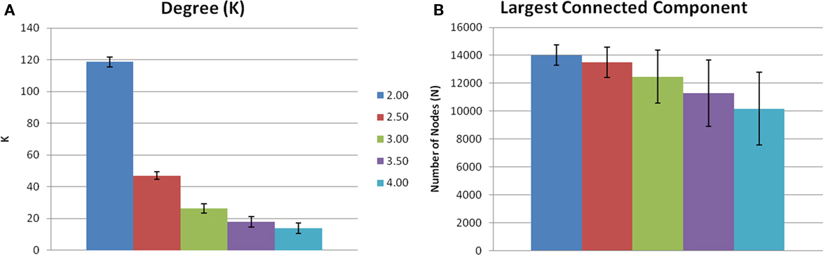
Figure 1. Threshold-dependent changes in network connectivity. (A) Shows the mean node degree across five thresholds. Mean degree was relatively consistent across thresholds 2.5–4.0. However, S = 2.0 there is an increase in mean degree indicating a loss of sparsity. (B) Is the number of voxels contained in the largest connected component. There is a gradual loss of nodes in the largest connected component as S increases.
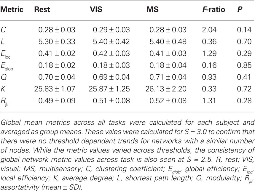
Table 1. Mean whole-brain network metrics for S = 3.0.
For each subject under each task whole-brain network metrics were generated for C, L, Eloc, Eglob, mean degree (K), modularity (Q), and assortativity (Rjk; Table 2). None of the metrics exhibited statistically significant differences between the rest, visual, or multisensory tasks. The ranges of each metric across tasks were: C (0.294–0.300), L (4.22–4.25), Eloc (0.48–0.49), Eglob (0.25–0.25), Q (0.65–0.66), K (46.91–47.40), and Rjk (0.44–0.48). Therefore, all whole-brain mean values exhibited no change across task.
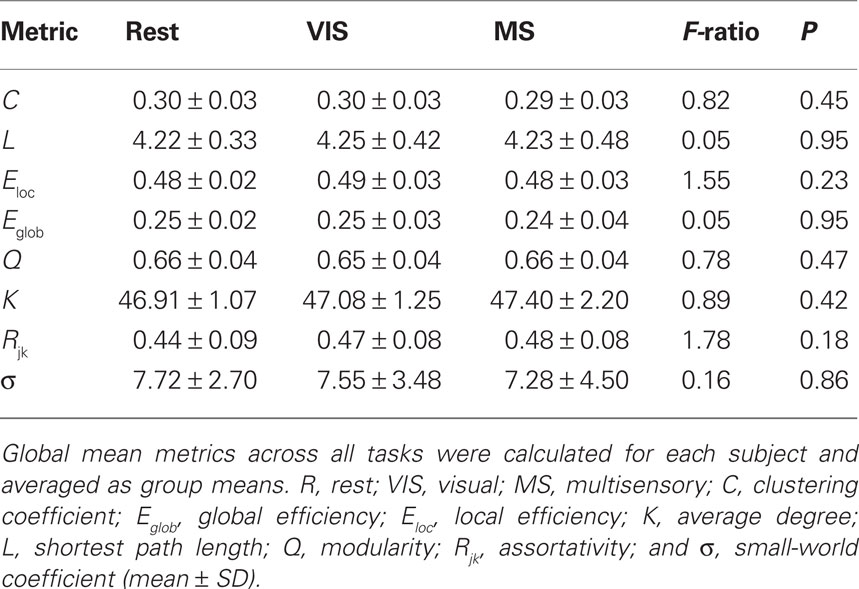
Table 2. Mean whole-brain network metrics for S = 2.5.
Small-world parameters were also assessed across conditions. For each group, sigma, σ, was calculated to determine the small-world-ness of each network (Condition, σ: rest, 7.72; visual, 7.55; multisensory, 7.29; Humphries and Gurney, 2008). All conditions were found to have small-world networks (σ > 1) and no significant differences were found across tasks (Table 2).
Analyses were performed to assess if the assortativity of a network was driven predominantly by high or low degree nodes. Rjk plots showing the distribution of connectivity demonstrated that regardless of condition all networks were assortative (Figure 2). It was also found that the assortativity of the networks were heavily driven by the lower degree nodes across the conditions (Figure 3).
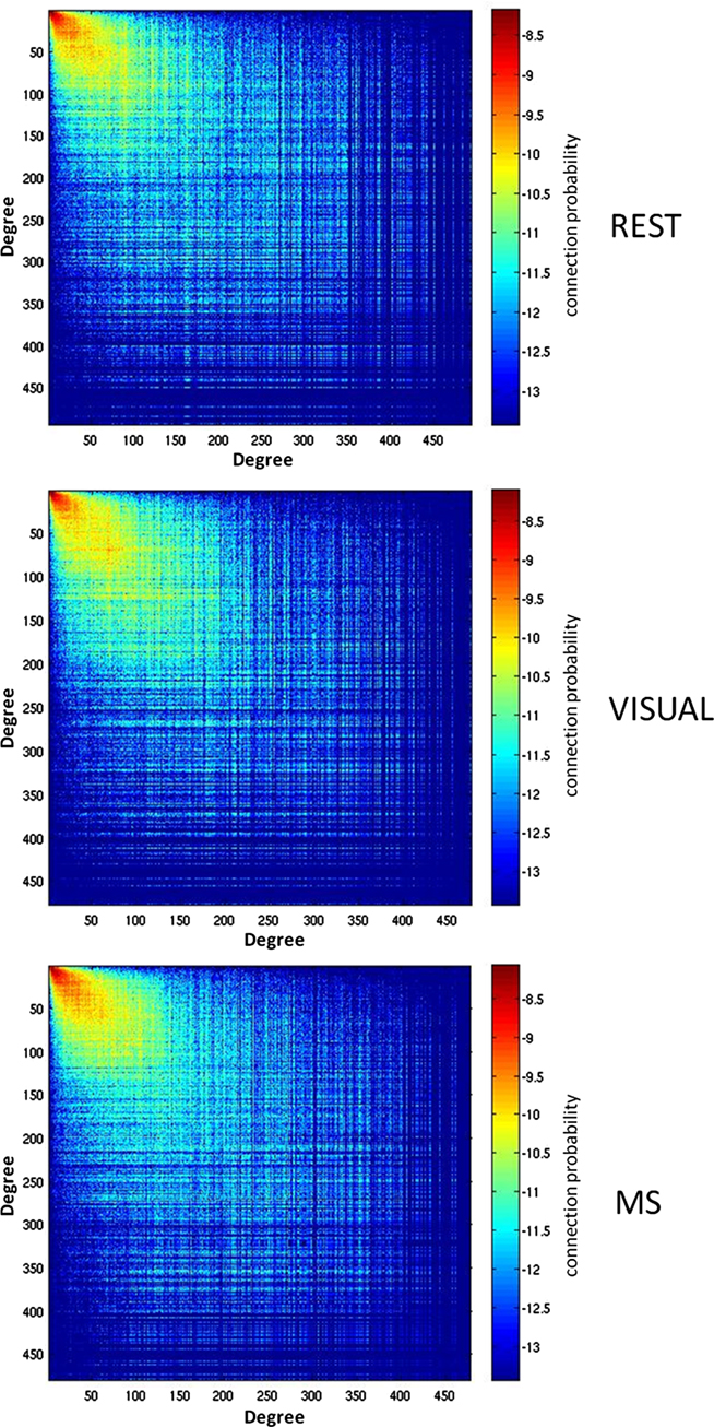
Figure 2. Assortativity of a representative subject. Assortativity (Rjk) for a single subject across all three conditions (rest, visual, and multisensory). The matrix depicts the degree of all connected nodes, generated by plotting the degree of each node on either end of each network edge. The warm region in the upper left corner of the plots denotes that the majority of network nodes have a low degree and are connected with other low degree nodes. The assortativity plots for the rest (REST), visual (VIS), and multisensory (MS) tasks all show a positive assortativity, in which nodes with similar degree are connected.
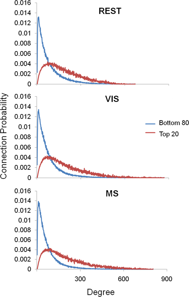
Figure 3. Assortativity sorted by degree. Above are the connection probabilities of the 80% lowest degree nodes and the top 20% highest degree nodes. For all three conditions rest (REST), visual (VIS), and multisensory (MS), the positive network assortativity was heavily weighted by low degree nodes. In each case, low degree nodes were connected with low degree nodes, peaking at nodes with a degree of around 25. On the other hand, high degree nodes’ connections were dispersed with a broad range of other degree nodes.
Degree distributions were plotted and exhibited exponentially truncated power law distributions across task (Figure 4). These data show that hubs exist despite the majority of nodes in the network having low degree. However, no obvious differences in these distributions across task were found.
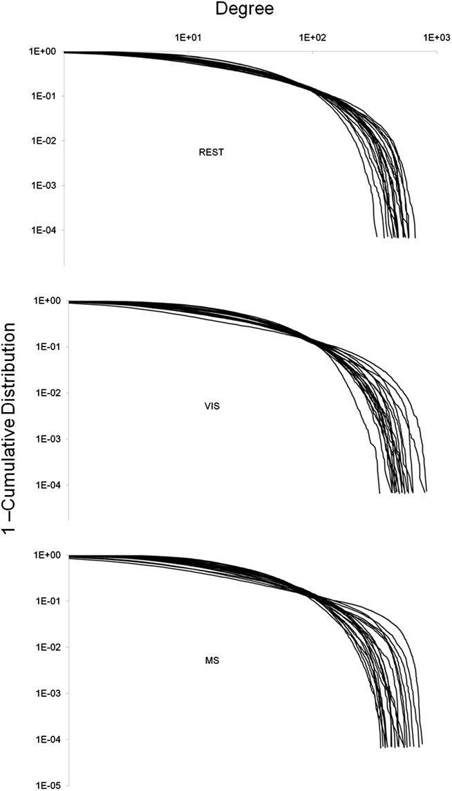
Figure 4. Whole-brain degree distributions. The degree of each node in a network was plotted against one minus the cumulative distribution. This was done for each individual in all three tasks: rest (REST), visual (VIS), and multisensory (MS). In all three cases, the degree distribution followed an exponentially truncated power law. No obvious differences between the tasks were observed.
Nodal Network Metrics
To investigate whether regional changes occurred despite consistency in whole-brain network means, the spatial distribution of network metrics was evaluated. Figures 5–7 show the top overlap maps of degree (K), local efficiency (Eloc), and global efficiency (Eglob), respectively. These maps exhibit the location and consistency across subjects of the individual nodes that are in the top 15% of all nodes for each individual metric. For example, the degree maps show the consistency of the top 15% of nodes with the largest number of connections. These results show that regional changes did occur across conditions. At rest, areas of the default mode network (DMN) exhibited the highest degree (Figure 5, REST). However, the prominence of the DMN decreased in the remaining tasks, with the greatest shifts observed in the multisensory condition. Note specifically that during the multisensory condition the precuneus/posterior cingulate cortex (PCC) was no longer among the most connected brain regions. The shifts exhibited task-driven changes that were consistent with the stimulus conditions. Connectivity (K) increased in the visual cortex during the visual task (Figure 5, VIS) and in both the visual and auditory cortices during the multisensory task (Figure 5, MS).
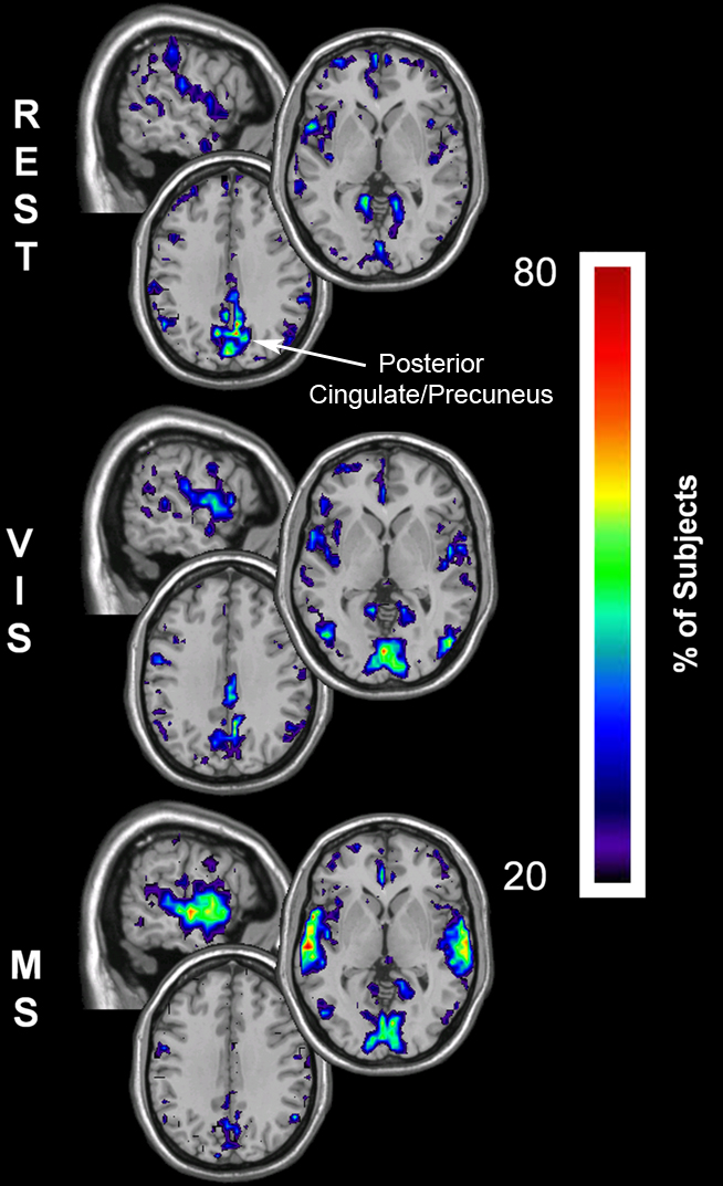
Figure 5. Degree overlay maps during rest, visual, and multisensory tasks. In each subject the voxels with degree values in the top 15% were identified. These maps represent the overlap of these voxels across subjects in each of the three tasks. The consistency of overlap between across subjects is indicated by the threshold color bar that which represents the percentage of individuals for which each voxel was among the top 15%. Degree maps show that at rest (REST) the parietal cortex has the greatest connectivity while the visual cortex has lower degree. There is a regional shift in degree during the visual task (VIS) to the visual cortex and to both the visual and auditory cortex during the multisensory task (MS).
To determine if these changes occurred both for local inter-connections (Eloc) as well as for long-distance communication (Eglob), efficiency maps were compared between tasks. Similar to the results found with degree, regional changes occurred across conditions for local efficiency (Figure 6). Local efficiency (clustering), during the resting state (Figure 6, REST) was greatest in the precuneus/PCC, a known region of the DMN related with information integration. Additionally, high clustering was found in the visual cortex, likely due to the visual fixation component of the rest task. During the visual task (Figure 6, VIS) there was a dynamic shift in clustering with greater local connectivity in the visual cortex and a decrease in the DMN regions. This trend was repeated in the multisensory condition, with a pronounced local connectivity increase in the visual cortex as well as in the auditory cortex (Figure 6, MS).
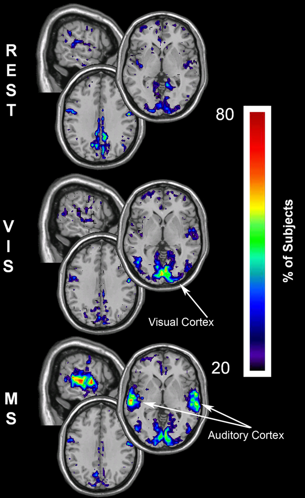
Figure 6. Local efficiency overlay maps during rest, visual, and multisensory tasks. In each subject the voxels with local efficiency values in the top 15% were identified. These maps represent the overlap of these voxels across subjects in each of the three tasks. The consistency of overlap across subjects is indicated by the threshold color bar that represents the percentage of individuals. Eloc maps show that at rest (REST) the visual and parietal cortices have the greatest clustering. Regions of high clustering shift during the visual task (VIS) to the visual cortex and to both the visual and auditory cortex during the multisensory task (MS). A progressive decrease in the local efficiency in the parietal cortex was observed across the three tasks.
The changes for global efficiency within the sensory cortices were less dramatic than those found for both degree and local efficiency. However, there was still a notable decrease in global efficiency within the PCC across tasks (Figure 7). These results show that the parietal lobe has the greatest global efficiency, which is equivalent to the shortest path length, in the rest condition. As shown with the other metrics this prominence is reduced in both the visual and multisensory tasks. Concurrently, there were increases in Eglob within the visual cortex during the visual task and in the visual and auditory cortices during the multisensory task.
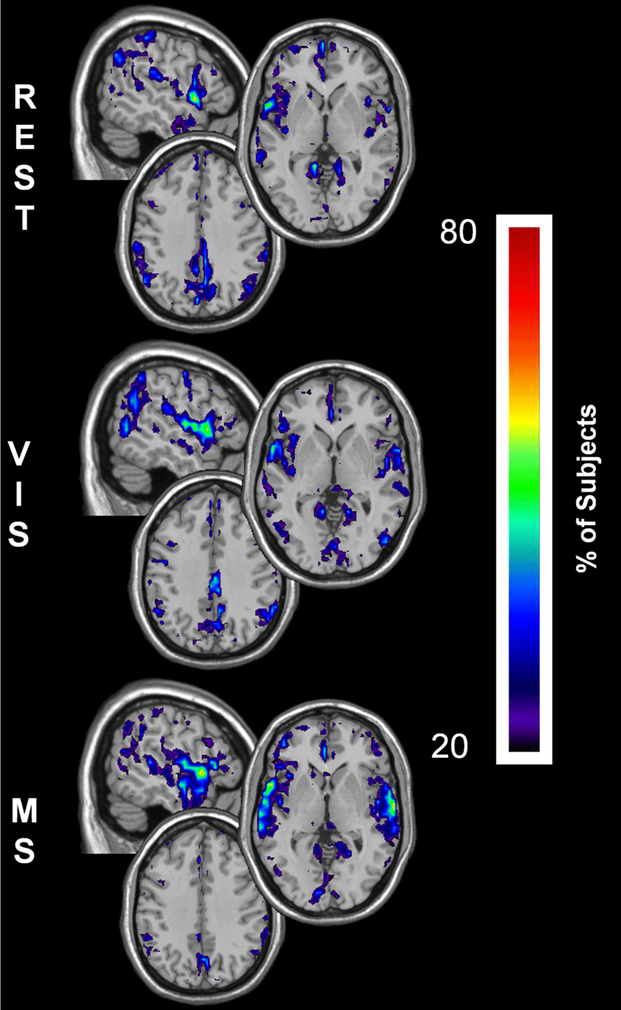
Figure 7. Global efficiency overlay maps, during rest, visual, and multisensory tasks. In each subject the voxels with global efficiency values in the top 15% were identified. These maps represent the overlap of these voxels across subjects in each of the three tasks. The consistency of overlap across subjects is indicated by the threshold color bar that represents the percentage of individuals. Eglob maps show that at rest (REST) the visual and parietal regions have the greatest across-network communication. There is a primary regional shift in global efficiency during the visual task (VIS) to the visual cortex and to both the visual and auditory cortices during the multisensory task (MS). In addition to this, there is a decrease in global efficiency within the parietal cortex across the three tasks. Note however, the relative change in the spatial location of high Eglob nodes was limited compared to K and Eloc.
Modular Structure of the Auditory Cortex
The overlap of each module containing the primary auditory cortex (bilateral Heschl’s gyri and the transverse temporal sulci) in all 20 individuals across all three tasks is shown in Figure 8. Of particular note is the spatial extent of these auditory modules across condition. In all three conditions, there is clear overlap in both the primary and secondary auditory cortices. However, auditory modules in the rest and visual conditions display much less specificity to the auditory cortex and also include brain regions not traditionally associated with audition, most notable the somatosensory cortices. When, however, the task begins to explicitly incorporate sound, as it does in the multisensory condition, the spatial extent of the auditory modules becomes more restricted to the auditory cortices. Interestingly, the extent of overlap across subjects also changes as a consequence of task with modest increases demonstrated in the visual condition but dramatic increases in the multisensory.
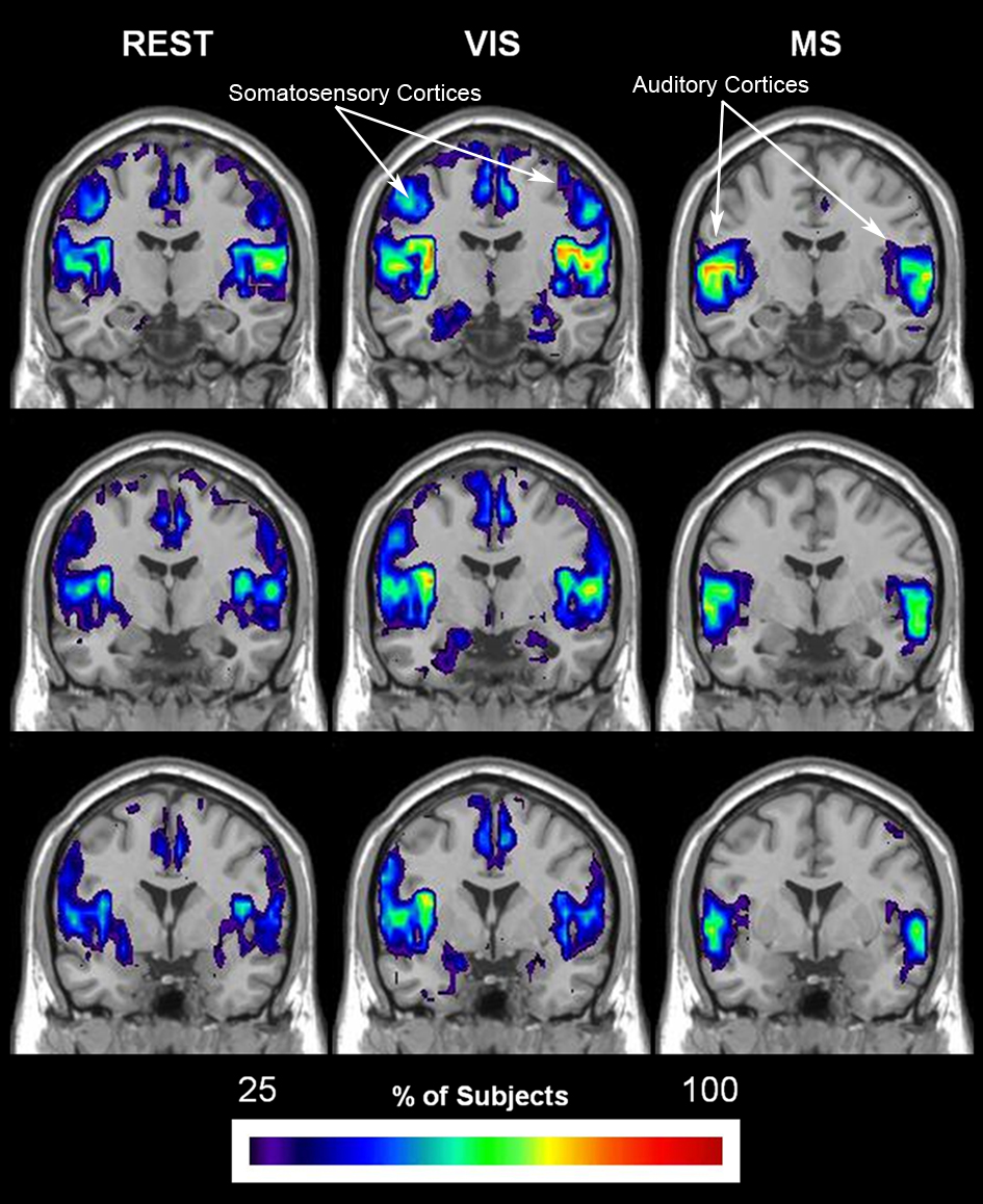
Figure 8. Change in spatial distribution of auditory module across task. The auditory module for each individual was selected using a mask that was defined by the primary auditory cortex, specifically bilateral Heschl’s gyri and transverse temporal sulci. After identification of the modules that encompassed auditory cortex in each individual, overlay images were generated for each task. Overlay images represent the summation of individual participant maps. The degree of overlay between these maps is indicated by the threshold color bar, which represents the percentage of participants. The spatial extent of the auditory module across tasks is shown to become more specific to both primary and secondary auditory cortices in the multisensory condition (MS). These modules, on the other hand, show less specificity to the auditory cortices in the conditions that do not have auditory stimulation: rest (REST) and visual (VIS).
Modular Structure of the Visual Cortex
The overlap of modules containing visual cortices (bilateral calcarine gyri, lingual gyri, occipital [(superior; middle; inferior) sulci and the cuneus] is shown for all three task conditions in Figure 9. In each condition, the spatial extent is restricted to visual areas. Although quite consistent across conditions, the group overlap in the visual cortex was notably greater in the visual and multisensory conditions as compared to rest.
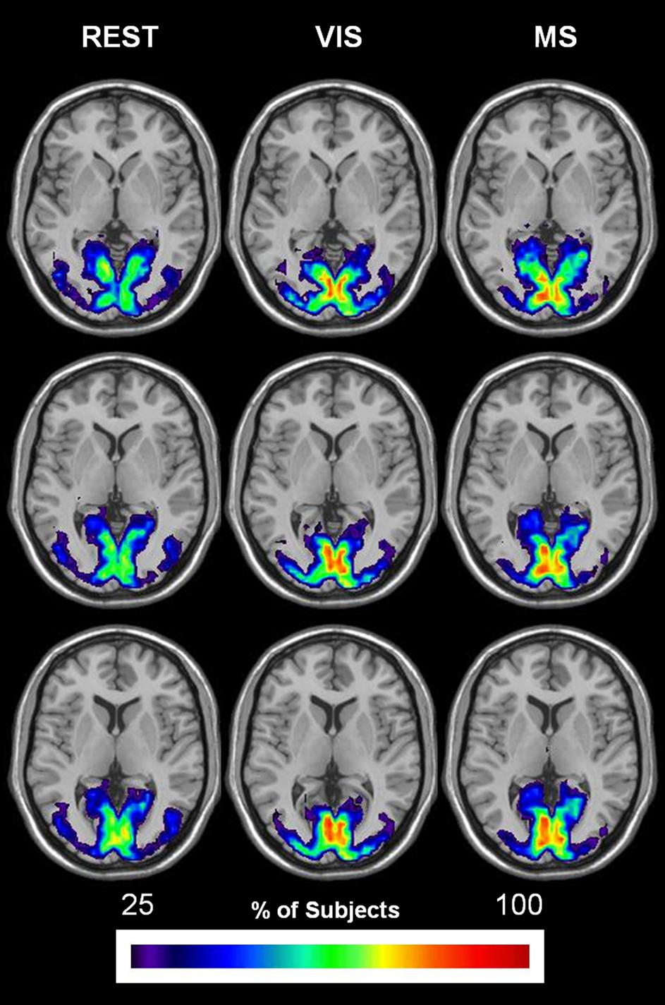
Figure 9. Change in spatial distribution of visual module across task. The same steps for generating auditory overlay maps were followed in order to create visual overlay maps. However, brain areas that composed the mask included: bilateral calcarine gyri, lingual gyri, occipital (superior; middle; inferior) sulci, and the cuneus. The spatial extent of the visual module across task is shown to remain relatively the same in all three conditions: rest (REST), visual (VIS), and multisensory (MS). Group overlap or consistency, on the other hand, exhibits an increase in both the visual and multisensory conditions.
Changes in the Network Topology of Auditory and Visual ROIs
Quantitative regional differences in measures of efficiency and degree were found across task in both the auditory and visual ROIs (Table 3). Of particular interest, no main effect of condition was found in Eglob, which is a network measure designed to capture global processing, in either region. This is similar to our previously stated findings that show generally consistent global network structure across different tasks. However, along with the regional modular differences already outlined, there were main effects of task in Eloc in both the auditory and visual ROIs and K in the auditory ROI. There was a trend for a main effect of condition on K in the visual ROI, however, this did not reach a statistical significance at p = 0.05. Regardless, it should be noted that these metrics capture more localized network structure and seem to be the most influenced by change in condition.
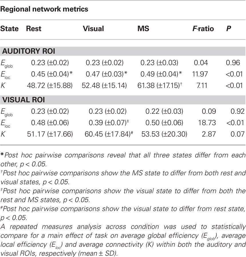
Table 3. Auditory and visual ROI metric assessment.
Whole-Brain Functional Cartography across Task
Spatial distribution of provincial hubs
Established methods of functional cartography (Guimera and Nunes Amaral, 2005; Joyce et al., 2010) were used to evaluate the spatial consistency of provincial and connector hubs. Provincial hubs, which have a pci ≤ 0.3, are high degree nodes that have the majority of their connections within their neighborhood and are thought to hold neighborhoods together. Connector hubs, which have a 0.3 < pci ≤ 0.75, are high degree nodes that have a substantial number of connections to other neighborhood and serve to interconnect neighborhoods. This analysis revealed that provincial hubs shifted spatial location across tasks (Figure 10). During the rest condition, the precuneus was the predominant provincial hub with high spatial overlap across subjects. A decrease in the provincial hub status of the precuneus during the visual condition was associated with an increase in the provincial hubs in the lateral visual cortices. Also, an even greater decrease in provincial hub status in the multisensory condition was observed in conjunction with provincial hubs in both the secondary visual and auditory cortices. Of particular note, these visual and multisensory-specific provincial hubs were absent in the rest condition. These data show that during the low level sensory input of the rest condition, the precuneus a predominant provincial hub. Moreover, they demonstrate that provincial hub status changes in accordance with task demand. Together, they suggest that brain networks, and in particular the role of individual nodes in maintaining modular organization, are dynamic in nature and can respond to external events in a task-dependent manner.
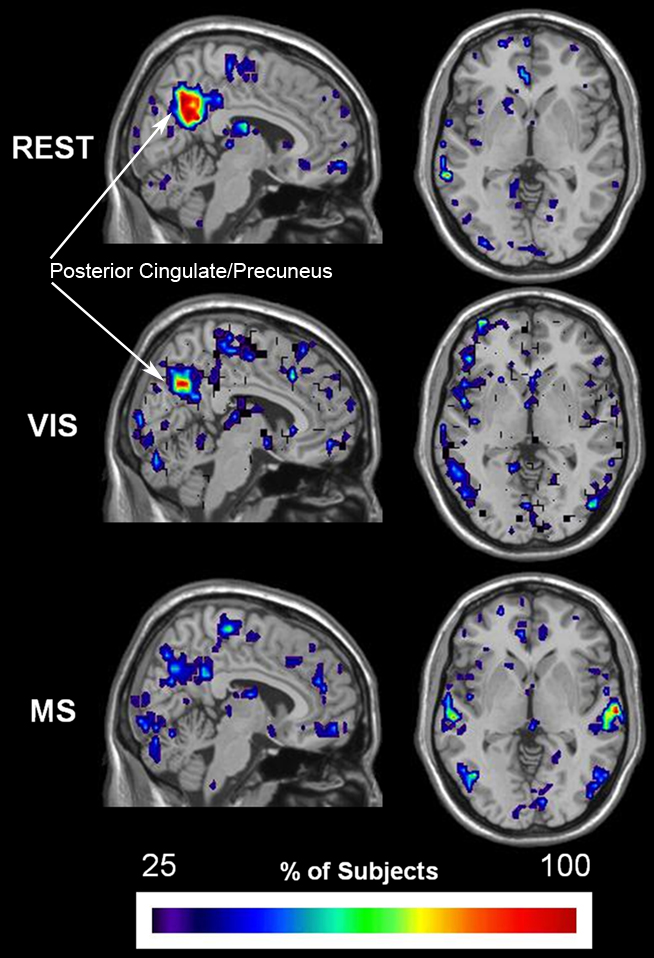
Figure 10. Change in spatial distribution of provincial hubs across tasks. Individual participant provincial hub (pki ≤ 0.01 and pci ≤ 0.3) maps were summated within each task to create an overlay image of spatial distribution within brain space. Note that the consistency of the provincial hubs is generally lower than the overlap presented in the preceding figures. However, there is a clear change in provincial node location across tasks. The rest (REST) condition shows with the greatest number and overlap of provincial hubs between participants in the precuneus, a brain region known to be part of the DMN. The number and overlap of provincial hubs in the visual and auditory cortices increases during the visual (VIS) and multisensory (MS) tasks. In addition, the precuneus loses provincial hubs during the sensory stimulation conditions.
Modular Functional Cartography across Task
Proportion of hub types
Significant differences in the proportion of provincial hubs (rest; visual; multisensory: 66; 80; 91%) and connector hubs (rest; visual; multisensory: 34; 20; 9%) within the auditory module across task were observed (Figure 11A). In this module, there was a main effect of task on the proportion of provincial hubs [yellow; task × node function: F(1, 19) = 6.6; p < 0.05] as well as the proportion of connectors [magenta; task × node function: F(1, 19) = 6.2; p < 0.05]. There was, however, no effect of task on the proportion of non-hubs (blue). These findings demonstrate that despite observed changes in the size of the auditory module across task (Figure 8); there exist real shifts in node function as a result of task demand. Furthermore, outside of non-hubs, it was found that there were predominately more connector hubs during the rest task (rest and visual: p = 0.05; rest and multisensory: p = 0.02) and more provincial hubs during the multisensory task (rest and visual: p = 0.04; rest and multisensory: p = 0.02). Contrary to the shift in node function within the auditory modules across task, no significant changes in the proportion of hubs or non-hubs in the visual cortex modules were observed (Figure 11B).
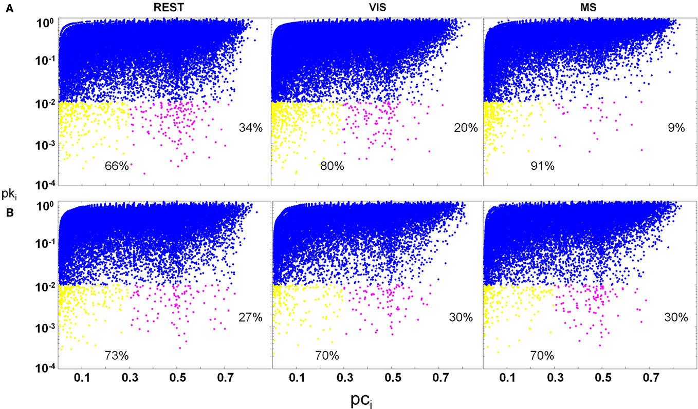
Figure 11. Change in hub proportions across task. Hubs are defined as having a pki ≤ 0.01. Provincial (yellow; pci ≤ 0.3) and connector (magenta; 0.3 < pci ≤ 0.75) hubs as well as non-hubs (blue; pki > 0.01) are plotted across task condition. In both auditory and visual modules, there was no change in the proportion of non-hubs across task. In the auditory module (A), a main effect of task was found for the proportion of hubs across condition. Connectors significantly decreased across task, with multisensory (MS) having the lowest proportion. In contrast, the proportion of provincial hubs increased across task, with rest (REST) having the lowest proportion. In the occipital module (B), no main effect of condition was found on the proportion of either hub type.
Discussion
There is an evergrowing movement toward framing questions of functional activity as questions that relate to interdependent systems. To do this in the brain, a model should capture qualities like distributive processing and localized specialization. In particular, information about the entire brain is necessary to best capture these properties. In the field of functional neuroimaging this has not been possible until the recent application of graph theory and the adoption of network science. Before this, attempts to model data as a system either involved seed or component-based analyses. In seed-based analyses a ROI acts as the starting point, or seed, from which a network is generated. As a consequence of focusing on one seed at a time information about the remaining portions of the brain and how they relate to the network in question is lost. Component-based analyses, on the other hand, are closer to capturing the information of the entire brain. These techniques separate functional information into components, or sub-networks, that are independent from each other. Consequently, these calculations show which areas in a brain are most strongly connected to other brain regions. Unfortunately, they do not give the researcher a sense of how many functional connections exist between different regions in a brain or between the different regions of one of its sub-networks.
Studies have unequivocally shown that functional connectivity is vulnerable to change when analyzed using either seed or component-based techniques (Jiang et al., 2004; Ma et al., 2011). These studies, however, do not explore whole-brain functional connectivity and whether or not it is changed by task or changes in cognitive state. In particular, because of the limitations discussed above, their results do not imply whatsoever that the functional connectivity of the entire brain is vulnerable to change. Interestingly, recent application of graph theory and network science to functional connectivity has shown that network topology, and in particular hub structure, is consistent regardless of task (Buckner et al., 2009). Though hub location may not be altered by changes in task, this study does not explore whether or not overall functional connectivity has been affected. For example, Buckner et al. (2009) showed the posterior cingulate to be an important hub during both passive and active task states. This finding, however, does not address if the brain regions functionally connected to the posterior cingulate have changed as a result of task. In our paper, we show that despite general consistency in network structure both qualitative and quantitative differences in regional network topology and functional connectivity arise as a consequence of task.
The application of graph theory to functional magnetic resonance imaging data has primarily focused on characterizing the brain using whole mean calculations (Bullmore and Sporns, 2009; He and Evans, 2010). In addition to this, the majority of these studies have been conducted with participants at rest (van den Heuvel et al., 2008). In the last few years a trend toward explaining networks throughout task performance has grown (Bassett et al., 2008; Feng et al., 2011; Xue et al., 2011; Yu et al., 2011). The resolution of nodes in these studies, however, is predominately based on 90-node atlas templates, which have been shown to be vulnerable to threshold effects that cause greater inter-subject variability and network fragmentation (Hayasaka and Laurienti, 2010). To the best of our knowledge, studies of functional connectivity that use both the principles of graph theory and a voxel-based approach during a complex task are extremely limited (Eguiluz et al., 2005). In this particular case, cause and effect trends were not readily interpretable because of the complexity of the task. Moreover, characterizations of regional shifts across tasks were limited in scope as the analyses focused primarily on node degree.
We show that when the principles of graph theory are applied to voxel-sized functional imaging data during rest and simple sensory conditions that regional network topology changes despite generally consistent overall network structure. In partial agreement with current literature (Buckner et al., 2009), we present results showing little change in whole-brain mean metric values across tasks (Table 2). However, contrary to prior results, in conducting a more comprehensive assessment of network structure we demonstrate that a full-scale analysis, which involves regional considerations, is necessary to understand the dynamic nature of functional connectivity throughout various conditions and/or cognitive states. The results presented herein demonstrate the utility of assessing the regional specificity of several metrics. These findings emphasize the dynamic nature of networks across task and are the first to show that voxel-based functional brain networks are dynamic and task-driven.
During rest, each metric identified the DMN, specifically the precuneus, as an important brain area. However, during the visual and multisensory tasks each metric exhibited shifts away from this important DMN region. Due to the consistency of the global values, the increases in connectivity, efficiency, and modularity within the visual and auditory cortices imply a decrease elsewhere within the network. Collectively, Figures 5–10 show this to be the case, with the precuneus connectivity decreasing with the addition of sensory stimuli. Therefore, regional metric shifts in brain networks can shed light on the functionality of brain areas during and across tasks.
One advantage of using network science to study the brain is the ability to model patterns of regional specificity and distributive properties with metrics such as Eloc, and Eglob. For example, an increased Eloc represents an increase in clustering and is indicative of brain regions with greater regional specificity. Because Eglob is the reciprocal of the characteristic path length, an increase in Eglob represents a shorter path length and therefore greater distributive properties or efficiency in information transfer. In these data, although average Eglob and Eloc remained consistent, the brain regions within the network with greatest regional specificity and distributive properties changed to brain regions involved with the given task (Figures 6 and 7).
To further support dynamic network interactions across task conditions, the community structure analyses presented here show that the visual and auditory modules exhibit greater spatial consistency and overlap during the visual and auditory tasks, respectively (Figures 8 and 9). For example, during the multisensory condition (Figure 8) the spatial extent of the auditory module across all individuals is primarily confined to the primary and secondary auditory cortices. To the contrary, in both the rest and visual conditions the auditory module also contains brain areas outside those traditionally known for audition. Interestingly, there is also an observed shift in the proportion of provincial and connector hubs within the auditory module across task, with the highest proportion of provincials exhibited in the multisensory condition (Figure 11A, MS) and the highest proportion of connectors in the rest condition (Figure 11A, REST). The enlarged auditory modules during rest, which include brain regions outside the auditory cortices as well as a large proportion of connector hubs, may help the person survey the environment for relevant information, and ready the brain in the event of an external demand. These findings suggest that when a cortical region is actively processing external information it becomes more inwardly focused and connections to other brain regions are shut down. Such changes in connectivity may provide mechanisms for task-tailored information processing.
These changes in modular consistency were accompanied by changes in local efficiency and degree (Table 3). It is of particular note to mention that Eloc captures localized topological changes in networks and is the metric most reliably changed by condition. This finding supports the notion that a more rigorous assessment of change between networks should include metrics that capture not only the distributed properties of brain structure but also its regionally segregated features.
The modular organization of the auditory cortex was highly focused and consistent across subjects during the multisensory task. The auditory modules were localized and confined to the primary and secondary auditory cortices (Figure 8, MS) and contained a greater proportion of provincial hubs than connector hubs (Figure 11A, MS). Together, these changes show that the auditory module has become more spatially specific in its information processing during multisensory feedback. Also, the functional role of connectors during this task, though still integrative in nature, may now be more directed so as to successfully process both visual and auditory information. Interestingly, a combination of the elements of modular organization seen in both the rest and multisensory tasks is nicely represented by that which is exhibited in the visual task (Figure 8, VIS). During this task, the auditory module is not as regionally descript as it is in the multisensory task and instead looks more similar to the auditory modules of the rest condition (Figure 8, REST). However, the provincial and connector hub proportions as well as the spatial overlap across subjects are more similar to that seen in the auditory modules of the multisensory task (Figure 8, MS). In the absence of a stimulus-relevant auditory signal, functional connectivity was organized in a way that could best synthesize the available input. To do this, auditory modules included other somatosensory cortices (Figure 8, VIS) and maintained a modest level of connector hubs (Figure 11A, VIS), which could sample information available in the rest of the network.
Neither the spatial extent nor the proportion of provincial and connector hubs in the visual module significantly changed across task (Figure 9). A likely explanation for this consistency lies in a combination of module choice and the nature of the visual tasks. In particular, despite there often being more than one visual module in a network, those modules with at least 10% of their nodes falling within the defined mask often represented primary visual cortices. Also, though sensory demand did change across task, with fixation being less visually demanding than watching a movie clip, primary visual processing, and the associated functional module is likely to be involved in all tasks. The spatial overlap across subjects did increase in both the visual and multisensory tasks possibly associated with the increased stimulus complexity. Ultimately, what is clear from this data is that with increases in sensory demand and stimulus complexity a greater number of individuals exhibit spatial coherence within the visual module and, therefore, also exhibit dynamic and responsive brain networks.
In the whole-brain functional cartography analyses of Figure 10, as sensory complexity increased from the rest to the multisensory condition, nodes within the precuneus, which is a commonly implicated DMN brain region, lost their provincial status. That is, they become increasingly less connected with other nodes in their modules. Interestingly, with this decrease in provincial node function within the precuneus there was a concurrent increase in provincial node function in those areas that are most likely to facilitate sensory processing in the visual and multisensory conditions: visual and auditory cortices. Again, as with the aforementioned findings, these results support that with task demand there is an associated change in network structure that likely facilitates overall information integration.
Collectively, these findings support the notion that brain networks have task-dependent dynamics. Moreover, they demonstrate how regional changes in network parameters may exist despite overall global consistency across conditions. Overall, our analyses in community structure underscore a common theme in these data: within various sensory conditions there are unique underlying networks that are dependent on the sensory load of the task. When we assess the nodes within these communities, or more specifically the modules within individual networks, a similar theme emerges. That is, a node’s function within modules changes depending on condition type.
Comparing networks across subjects and tasks is an obstacle with inherent limitations. In the current state of research, the easiest and most widely used method of evaluating and comparing networks has been through the use of mean whole-brain metric values that are statistically compared across subjects to test for change. There are two inherent problems with this approach. First, the choice of metrics may potentially influence the observed findings. That is, the metrics of any one study may not be sufficiently sensitive to capture change. Second, and as this paper demonstrates, the resolution used to study networks will also undoubtedly bias results. In light of these limitations, this study compared networks on an extensive list of network parameters and did so at two resolutions: the whole-brain and nodal level.
It should be noted that the methodology behind quantifying regional differences in networks that are generated under the principles of graph theory is far from being well established. Recently, edge-based statistical techniques (Fornito et al., 2011) and exponential random graph modeling approaches (Simpson et al., 2011) have moved the field toward more systematic ways of quantifying network differences between groups of individuals. The qualitative differences exhibited in Figures 5–10, however, are quite suggestive of quantitative differences in network structure as a result of condition. The dilemma researchers are then left with is how to best capture this change using an already firmly established statistical framework. To do so, these analyses focused on the differences among the means of network metrics within a region of interest across task condition. In the future, statistical approaches that are better tailored to the nature of network metric distributions will need to be used to more accurately address not only regional differences but also whole-brain.
The absence of an isolated auditory condition was a limitation of this study. This shortcoming was due to the lack of multisensory stimuli that can be broken down into both a visual and an auditory component, while still maintain meaning. Many studies have used the combination of visual and auditory stimuli such as a flashing checkerboard along with a tone to assess multisensory processing. However, while this combination cues both visual and auditory cortices it does not have a dualistic component that tests higher level multisensory processing. Therefore, this study chose to use a more complex stimulus to address a true multisensory state. Unfortunately, there was not an auditory clip long enough in the movie that could be used for an auditory-only condition. If segments of the movie were concatenated so that there was a 5.6 minutes long auditory clip, we felt it would have lost contextual relevance. As a consequence, these analyses do not explore changes in network structure as result of audition and, thus, do not directly address its potential influence on networks observed in the multisensory condition. Future studies characterizing the effect of audition on network structure are needed, particularly for those research questions that are related to multisensory integration.
A high-resolution correlation matrix will increase network specificity. Unfortunately, higher resolution matrices come at the cost of a lower signal to noise ratio. To strike a balance between networks that are overly dense and likely to mask regional shifts in network metrics and those that are too sparse and insensitive to regional shifts, a threshold needs to be applied to network data. This threshold is ultimately arbitrary in nature; however, research with brain networks has offered some direction (Hayasaka and Laurienti, 2010). Though the analyses presented here were not threshold-dependent, it would be of great benefit to the field if a systematic means of thresholding networks were developed.
Taken together our findings support one overarching theme: networks are dynamic and undoubtedly influenced by the nature of stimuli presentation. Despite stability in whole-brain metric values across condition, we have found that a more comprehensive analysis of network structure is essential in understanding the dynamics of functional connectivity networks. More importantly, this assessment must include a regional survey of the spatial distribution of network parameters.
Conflict of Interest Statement
The authors declare that the research was conducted in the absence of any commercial or financial relationships that could be construed as a potential conflict of interest.
Acknowledgments
This work was supported by National Institute of Neurological Disorders and Stroke at the National Institutes of Health (NS042568 and NS070917); the Wake Forest University General Clinic Research Center (RR07122); the Roena Kulynych Memory and Cognition Research Center; and the Translational Science Center at the Reynolda Campus of Wake Forest University.
Footnotes
References
Babor, T. F., Higgins-Biddle, J. C., Saunders, J. B., and Monteiro, M. G. (2001). AUDIT: The Alcohol Use Disorders Identification Test: Guidelines for Use in Primary Care. 2nd Edn. World Health Organization, Geneva.
Bassett, D. S., Bullmore, E., Verchinski, B. A., Mattay, V. S., Weinberger, D. R., and Meyer-Lindenberg, A. (2008). Hierarchical organization of human cortical networks in health and schizophrenia. J. Neurosci. 28, 9239–9248.
Beckmann, C. F., DeLuca, M., Devlin, J. T., and Smith, S. M. (2005). Investigations into resting-state connectivity using independent component analysis. Philos. Trans. R. Soc. Lond. B Biol. Sci. 360, 1001–1013.
Biswal, B., Yetkin, F. Z., Haughton, V. M., and Hyde, J. S. (1995). Functional connectivity in the motor cortex of resting human brain using echo-planar MRI. Magn. Reson. Med. 34, 537–541.
Buckner, R. L., Sepulcre, J., Talukdar, T., Krienen, F. M., Liu, H., Hedden, T., Andrews-Hanna, J. R., Sperling, R. A., and Johnson, K. A. (2009). Cortical hubs revealed by intrinsic functional connectivity: mapping, assessment of stability, and relation to Alzheimer’s disease. J. Neurosci. 29, 1860–1873.
Bullmore, E., and Sporns, O. (2009). Complex brain networks: graph theoretical analysis of structural and functional systems. Nat. Rev. Neurosci. 10, 186–198.
Calhoun, V. D., Adali, T., Pearlson, G. D., and Pekar, J. J. (2001). Spatial and temporal independent component analysis of functional MRI data containing a pair of task-related waveforms. Hum. Brain Mapp. 13, 43–53.
Calhoun, V. D., Pekar, J. J., McGinty, V. B., Adali, T., Watson, T. D., and Pearlson, G. D. (2002). Different activation dynamics in multiple neural systems during simulated driving. Hum. Brain Mapp. 16, 158–167.
Colcombe, S., and Kramer, A. F. (2003). Fitness effects on the cognitive function of older adults: a meta-analytic study. Psychol. Sci. 14, 125–130.
De Luca, M., Beckmann, C. F., De Stefano, N., Matthews, P. M., and Smith, S. M. (2006). fMRI resting state networks define distinct modes of long-distance interactions in the human brain. Neuroimage 29, 1359–1367.
Eguiluz, V. M., Chialvo, D. R., Cecchi, G. A., Baliki, M., and Apkarian, A. V. (2005). Scale-free brain functional networks. Phys. Rev. Lett. 94, 018102.
Feng, Y., Bai, L., Ren, Y., Wang, H., Liu, Z., Zhang, W., and Tian, J. (2011). Investigation of the large-scale functional brain networks modulated by acupuncture. Magn. Reson. Imaging 34, 31–42.
Folstein, M. F., Folstein, S. E., and McHugh, P. R. (1975). “Mini-mental state.” A practical method for grading the cognitive state of patients for the clinician. J. Psychiatr. Res. 12, 189–198.
Fornito, A., Yoon, J., Zalesky, A., Bullmore, E. T., and Carter, C. S. (2011). General and specific functional connectivity disturbances in first-episode schizophrenia during cognitive control performance. Biol. Psychiatry 70, 64–72.
Freeman, L. C. (1979). Centrality in social networks: conceptual clarification. Soc. Networks 1, 215–239.
Girvan, M., and Newman, M. E. (2002). Community structure in social and biological networks. Proc. Natl. Acad. Sci. U.S.A. 99, 7821–7826.
Guimera, R., and Nunes Amaral, L. A. (2005). Functional cartography of complex metabolic networks. Nature 433, 895–900.
Hampson, M., Tokoglu, F., Sun, Z., Schafer, R. J., Skudlarski, P., Gore, J. C., and Constable, R. T. (2006). Connectivity-behavior analysis reveals that functional connectivity between left BA39 and Broca’s area varies with reading ability. Neuroimage 31, 513–519.
Hayasaka, S., and Laurienti, P. J. (2010). Comparison of characteristics between region-and voxel-based network analyses in resting-state fMRI data. Neuroimage 50, 499–508.
He, Y., and Evans, A. (2010). Graph theoretical modeling of brain connectivity. Curr. Opin. Neurol. 23, 341–350.
Hugenschmidt, C. E., Mozolic, J. L., Tan, H., Kraft, R. A., and Laurienti, P. J. (2009). Age-related increase in cross-sensory noise in resting and steady-state cerebral perfusion. Brain Topogr. 21, 241–251.
Humphries, M. D., and Gurney, K. (2008). Network “small-world-ness”: a quantitative method for determining canonical network equivalence. PLoS ONE 3, e0002051. doi: 10.1371/journal.pone.0002051
Jafri, M. J., Pearlson, G. D., Stevens, M., and Calhoun, V. D. (2008). A method for functional network connectivity among spatially independent resting-state components in schizophrenia. Neuroimage 39, 1666–1681.
Jiang, T., He, Y., Zang, Y., and Weng, X. (2004). Modulation of functional connectivity during the resting state and the motor task. Hum. Brain Mapp. 22, 63–71.
Joyce, K. E., Laurienti, P. J., Burdette, J. H., and Hayasaka, S. (2010). A new measure of centrality for brain networks. PLoS ONE 5, e12200. doi: 10.1371/journal.pone.0012200
Latora, V., and Marchiori, M. (2001). Efficient behavior of small-world networks. Phys. Rev. Lett. 87, 198701.
Ma, L., Steinberg, J. L., Hasan, K. M., Narayana, P. A., Kramer, L. A., and Moeller, F. G. (2011). Working memory load modulation of parieto-frontal connections: evidence from dynamic causal modeling. Hum. Brain Mapp. doi: 10.1002/hbm.21329. [Epub ahead of print].
Maldjian, J. A., Laurienti, P. J., Kraft, R. A., and Burdette, J. H. (2003). An automated method for neuroanatomic and cytoarchitectonic atlas-based interrogation of fMRI data sets. Neuroimage 19, 1233–1239.
Maslov, S., and Sneppen, K. (2002). Specificity and stability in topology of protein networks. Science 286, 910–913.
McKeown, M. J., Makeig, S., Brown, G. G., Jung, T. P., Kindermann, S. S., Bell, A. J., and Sejnowski, T. J. (1998). Analysis of fMRI data by blind separation into independent spatial components. Hum. Brain Mapp. 6, 160–188.
Michael, A. M., Calhoun, V. D., Andreasen, N. C., and Baum, S. A. (2008). A method to classify schizophrenia using inter-task spatial correlations of functional brain images. Conf. Proc. IEEE Eng. Med. Biol. Soc. 2008, 5510–5513.
Newman, M. E. (2003b). Mixing patterns in networks. Phys. Rev. E Stat. Nonlin. Soft Matter Phys. 67, 026126.
Newman, M. E., and Girvan, M. (2004). Finding and evaluating community structure in networks. Phys. Rev. E Stat. Nonlin. Soft Matter Phys. 69, 026113.
Newman, M. E. J. (2008) “Mathematics of networks,” in The New Palgrave Dictionary of Economics, 2nd Edn, Eds. N. S. Durlauf and L. E. Blume Basingstoke: Palgrave Macmillan. Available at: http://www.dictionaryofeconomics.com/article?id=pde2008_M000361 [August 03, 2011].
Radloff, L. S. (1977). The CES-D scale: a self-reported depression scale for research in the general population. Appl. Phychol. Meas. 1, 385–401.
Raichle, M. E., MacLeod, A. M., Snyder, A. Z., Powers, W. J., Gusnard, D. A., and Shulman, G. L. (2001). A default mode of brain function. Proc. Natl. Acad. Sci. U.S.A. 98, 676–682.
Ruan, J., and Zhang, W. (2008). Identifying network communities with a high resolution. Phys. Rev. E Stat. Nonlin. Soft Matter Phys. 77, 016104.
Rubinov, M., and Sporns, O. (2010). Complex network measures of brain connectivity: uses and interpretations. Neuroimage 52, 1059–1069.
Simpson, S. L., Hayasaka, S., and Laurienti, P. J. (2011). Exponential random graph modeling for complex brain networks. PLoS ONE 6, e20039. doi: 10.1371/journal.pone.0020039
Stam, C. J., and Reijneveld, J. C. (2007). Graph theoretical analysis of complex networks in the brain. Nonlinear Biomed. Phys. 1, 3.
Tzourio-Mazoyer, N., Landeau, B., Papathanassiou, D., Crivello, F., Etard, O., Delcroix, N., Mazoyer, B., and Joliot, M. (2002). Automated anatomical labeling of activations in SPM using a macroscopic anatomical parcellation of the MNI MRI single-subject brain. Neuroimage 15, 273–289.
van de Ven, V. G., Formisano, E., Prvulovic, D., Roeder, C. H., and Linden, D. E. (2004). Functional connectivity as revealed by spatial independent component analysis of fMRI measurements during rest. Hum. Brain Mapp. 22, 165–178.
van den Heuvel, M. P., Stam, C. J., Boersma, M., and Hulshoff Pol, H. E. (2008). Small-world and scale-free organization of voxel-based resting-state functional connectivity in the human brain. Neuroimage 43, 528–539.
Watts, D. J., and Strogatz, S. H. (1998). Collective dynamics of ‘small-world’ networks. Nature 393, 440–442.
Xue, S., Tang, Y. Y., and Posner, M. I. (2011). Short-term meditation increases network efficiency of the anterior cingulate cortex. Neuroreport. 22, 570–574.
Keywords: network science, task-based, small-world, efficiency, modularity
Citation: Moussa MN, Vechlekar CD, Burdette JH, Steen MR, Hugenschmidt CE and Laurienti PJ (2011) Changes in cognitive state alter human functional brain networks. Front. Hum. Neurosci. 5:83. doi: 10.3389/fnhum.2011.00083
Received: 21 March 2011;
Accepted: 28 July 2011;
Published online: 22 August 2011.
Edited by:
Hauke R. Heekeren, Max Planck Institute for Human Development, GermanyReviewed by:
Leighton B. Hinkley, University of California San Francisco, USADaniel S. Margulies, Max Planck Institute, Germany
Copyright: © 2011 Moussa, Vechlekar, Burdette, Steen, Hugenschmidt and Laurienti. This is an open-access article subject to a non-exclusive license between the authors and Frontiers Media SA, which permits use, distribution and reproduction in other forums, provided the original authors and source are credited and other Frontiers conditions are complied with.
*Correspondence: Malaak Nasser Moussa, Neuroscience Program, Laboratory for Complex Brain Networks, Medical Center Boulevard, Wake Forest University School of Medicine, Winston-Salem, NC 27157-1083, USA. e-mail: mamoussa@wfubmc.edu