

Abstract
In this paper we construct, on the basis of existing experimental data, a mathematical model of firing-elicited release of peptide transmitters from motor neuron B15 in the accessory radula closer neuromuscular system of Aplysia. The model consists of a slow “mobilizing” reaction and the fast release reaction itself. Experimentally, however, it was possible to measure only the mean, heavily averaged release, lacking fast kinetic information. Considered in the conventional way, the data were insufficient to completely specify the details of the model, in particular the relative properties of the slow and the unobservable fast reaction. We illustrate here, with our model and with additional experiments, how to approach such a problem by considering another dimension of release, namely its pattern dependence. The mean release is sensitive to the temporal pattern of firing, even to pattern on time scales much faster than the time scale on which the release is averaged. The mean release varies with the time scale and magnitude of the pattern, relative to the time scale and nonlinearity of the release reactions with which the pattern interacts. The type and magnitude of pattern dependence, especially when correlated systematically over a range of patterns, can therefore yield information about the properties of the release reactions. Thus, temporal pattern can be used as a probe of the release process, even of its fast, directly unobservable components. More generally, the analysis provides insights into the possible ways in which such pattern dependence, widespread especially in neuropeptide- and hormone-releasing systems, might arise from the properties of the underlying cellular reactions.
- synaptic transmission
- neurotransmitter
- neuropeptide
- transmitter release
- firing pattern
- temporal pattern dependence
- mathematical modeling
- Aplysia
Release of neurotransmitters and hormones is brought about by a complex sequence of intracellular reactions with differing kinetics and stimulation dependence (for review, see Zucker, 1996; Neher, 1998;Kasai, 1999). The dynamic interplay of these reactions underlies the plasticity with which the release responds in a functionally appropriate manner to different patterns and histories of stimulation (Fisher et al., 1997; O'Donovan and Rinzel, 1997). For functional prediction of release, as well as to aid in identification of the underlying molecular machinery, it is therefore highly desirable to obtain a quantitative understanding of the properties of the release reactions and their mutual relations, such as may be embodied in a mathematical model (Magleby and Zengel, 1982; Heinemann et al., 1993;Dittman et al., 2000). Considerable progress in this direction has been made in preparations where release can be measured in “real time,” with high temporal resolution, using a fast electrophysiological response to the released transmitter or a capacitance, amperometric, or optical measure of exocytosis (Angleson and Betz, 1997; Neher, 1998). As schematized in Fig. 1, these techniques allow direct observation of the detailed waveform of release (second row frombottom) that results from any pattern of stimulation (second row from top).
In many interesting preparations, however, these techniques cannot be easily applied. In this paper we deal with one such system: release of peptide transmitters from motor neuron B15 in the accessory radula closer (ARC) neuromuscular system of Aplysia. This release was measured in a series of studies by Vilim and colleagues (Vilim, 1993; Vilim et al., 1996a,1996b); we begin here by modeling their data. Because the functional consequences of the release for the whole, intact system are of major interest (Weiss et al., 1993; Brezina et al., 1996), release was studied in the intact system, from B15 terminals lying inaccessible within the muscle. There is no fast electrophysiological response to these modulatory transmitters. The amounts released are small, and the radioimmunoassay (RIA) technique used by Vilim et al. (1996a,b) integrated the amounts over intervals of several minutes. Thus, rather than the detailed waveform of the release, Vilim et al. (1996a,b) could only measure the mean, heavily averaged release (see Fig. 1, bottom row).
Nevertheless, as we illustrate here using our model and with additional experiments, such measurements can provide considerable information about the properties of the release process. This is because the mean release, in general, is sensitive to the temporal pattern of the stimulation—the way in which a given “amount” of stimulation is arranged in time, even on time scales that may be much faster than that on which the release is averaged. For example, the pattern schematized in the right column of Figure 1 gives threefold greater mean release than the middle pattern, although both patterns deliver the same amount of stimulation (top row). Knowing the general rules that govern such pattern dependence (Brezina et al., 1997), its type and magnitude yield information about the properties of the release reactions that generated it. Temporal pattern can thus be used as a probe of the release process.
Release of transmitters and hormones is strongly pattern dependent in many systems, with important physiological consequences (Dutton and Dyball, 1979; Andersson et al., 1982;Ip and Zigmond, 1984; Cazalis et al., 1985; Bicknell, 1988; Birks and Isacoff, 1988; Peng and Horn, 1991). It is therefore of considerable interest to see how pattern dependence arises from the properties of the underlying intracellular reactions, so as to be able to understand when different types of pattern dependence can and cannot arise.
MATERIALS AND METHODS
Modeling
Here we describe important aspects of the modeling in more technical detail than could be given in the general overview in Results. The principal variables, parameters, and symbols used are summarized in Table 1.
Firing patterns
Vilim et al. (1996a,b) used regular repetitive bursting patterns of the kind shown in Figure 2A. In addition to the total stimulation length L, such patterns are completely definable by three parameters such as the burst duration dintra, the interburst interval dinter, and the intraburst firing frequency fintra, or equivalently the cycle period P = dintra + dinter, the duty cycle D = dintra/ P, and the mean firing frequency 〈f〉 = fintraD (Brezina et al., 1997, 2000). Figure2A is drawn to scale to show the values that Vilim et al. (1996a,b) used as a standard reference pattern: dintra = 3.5 sec, dinter = 3.5 sec, fintra = 12 Hz; or equivalently P = 7 sec, D = 0.5, 〈f〉 = 6 Hz; L = 1 hr.
The waveform of firing frequency f at time t can be conveniently expressed as:
 Equation 1where t mod P is the remainder after dividing P into t the largest possible integral number of times. For simplicity, we will use “ f(t) ” to refer, as well as to the value of f at a particular time t, to a section, or the whole waveform of such values.
The special case dinter = 0 or D = 1 represents “unpatterned,” tonic firing, expressible as:
 Equation 2For every patterned f(t) described by Equation 1there exists unpatterned firing described by Equation 2 with the same mean frequency. We denote this f′(t).
Model equations
A general model with the required properties (see Basic model of the release data of Vilim et al. in Results) is given by the equations:
 Equation 3a
 Equation 3b
 Equation 3c
Below we analyze and fit to the data two versions of the model, setting a priori either y = 1 (Model I) or x = 1 (Model II).
Model I: y = 1
Analysis. Model I gives essentially pattern-independent release with all of the patterns used byVilim et al. (1996a,b) (see Pattern dependence generated by Models I and II in Results). For the purposes of reproducing the release measured by Vilim et al. (1996a,b), averaged on a time scale much longer than P, we may therefore replace every patterned f(t) given by Equation 1 with the equivalent unpatterned f′(t) given by Equation 2.
Equation 3b can then be alternatively written as:
 Equation 4where:
 Equation 5ais the steady-state value that p(t) approaches as t → L, with “dissociation constant” Kp ≡ kp−/ kp+, and
 Equation 5bis the time constant of relaxation to the steady state.
We note that Equation 3a potentially allows rapid release of all S . In the data of Vilim et al. (1996a,b), however, S(t) decreases only slowly as the firing continues (see Fig.2B). This means that p(t)x, and p(t) itself, must be small. Hence 1 − p(t) ≈ 1 in Equation 3b, and Equations 5a and 5b simplify to
 Equation 6a.b
For f′(t) given by Equation 2, with p(0) = 0 and S(0) = S, and with y = 1 and x = 4 (determined below to be the integral value that best fits the data), Equations 3 and 4 have the analytical solutions:
 Equation 7a
 Equation 7b
 Equation 7cwhere a(t) = t −
 τp + τp[4 exp (−t/τp) − 3 exp (−2t/τp) +
 exp (−3t/τp) − ¼ exp (−4t/τp)].
Finally, if we define:
 Equation 8the total amount released up to time t, clearly:
 Equation 9
Fitting the model to the data. Ideally, r(t) given by Equation 7a could now be fitted to the data. However, Vilim et al. (1996a,b) did not directly measure r(t), but rather outflow from the muscle, o(t), i.e., r(t) transformed by some transport function δT, which we do not know a priori. Nevertheless,Vilim et al. (1996a,b) presented two kinds of data that together provided a way past this problem.
[In the data of Vilim et al. (1996a,b), small cardioactive peptide (SCP) and buccalin (BUC) release appears indistinguishable in all respects except absolute amounts (see Figs. 2B, 3, 4) (see Basic model of the release data of Vilim et al. in Results). For fitting, we therefore always pooled SCP and BUC data or constrained the fit to yield identical parameter values, except absolute amounts.]
(1) Long L (1 hr). These data are reproduced in Figure2B. The transport function δT can be thought of as being composed, roughly, of a “diffusional” component δD and a “bulk-flow” component δB, which slow and retard, respectively, o with respect to r. [In the interpretation of the model, the tail of o(t > L) in Fig. 2B, when according to Eq. 7a r(t > L) = 0, is a direct reflection of δT; the complete effect of δT can be seen in Fig. 5C.] After a sufficiently long time into the block of firing L, t > τp, p(t) → p∞, r(t) changes slowly, and δD can be assumed to be near steady state. [This is strictly true, of course, only if we have substituted the unpatterned f′(t).] Then release should directly appear as outflow, but with some fixed delay τB, the mean transit time out of the muscle by the bulk-flow process δB. Using Equation 7a, we predict:
 Equation 10Indeed, as Figure 2B shows, the decline of o(t > 20 min) was well fit by a single exponential with rate constant of 0.037 min−1 (time constant of ∼27 min). By Equation 10, the rate constant is equal to p∞4〈f〉. Thus p∞(〈f〉 = 6 Hz) ≈ 0.10. Then, using Equation 5a, Kp ≈ 54 sec−1.
(2) Short L (5–10 min). In these experiments the system did not have time to reach steady state; no simplifying assumption about δT can be made to extract r(t) from o(t). Thus the time course of o is not useful in this case. Instead, Vilim et al. (1996a,b) measured the total peptide outflow resulting from the whole block of firing of length L, O∞(L) —i.e., not only the outflow during L itself, but also the tail of outflow afterward (see Fig.8A). We define:
 Equation 11Experiments were performed with different patterns over fixed L = 10 min. Because with the patterns used Model I gives pattern-independent release, and Vilim et al. (1996a,b) indeed apparently observed O∞ dependent simply on 〈f〉 (see Experimental test of the pattern dependence predicted by Models I and II in Results), all of these data are replotted together against 〈f〉 in Figure 3A. Other experiments were performed with fixed pattern but varying L (see Fig. 3B).
From Equations 7c and 9, we find:
 Equation 12Equation 12 (together with Equations 5) was simultaneously fitted to the data in Figure 3, A and B, using the value of Kp from the long- L data. As Figure 3, A and B, shows (solid curves), this fit, with x = 4, was excellent. A similar fitting was carried out for x = 1, 2, 3, and 5, using the appropriate equivalent of Equation 12 [differing in the exponent of p∞ and the terms of a(L)] and appropriately recalculated Kp. However, each of these fits was inferior to that obtained with x = 4. The fits with x = 1, 2, and 3 had too little curvature; the fit with x = 5 had too much curvature (Fig. 3A, B, dashed curves).
The inset of Figure 3B extends the time axis to longer L and confirms that the best fit to the short- L data also fits the total outflow in the long- L experiments.
These fits yielded the values kp+ = 2.04 × 10⁻⁴, kp−= 1.10 × 10⁻² sec−1, S0,SCP = 542 fmol, and S0,BUC = 200 fmol. The S0 values are indicated in Figure 3B,inset, and discussed further below.
Model II: x = 1
Analysis. In Model II, for all of the patterns used by Vilim et al. (1996a,b), significant pattern dependence is generated only by the nonlinearityf(t)y (see Pattern dependence generated by Models I and II in Results). For the purposes of reproducing the release measured by Vilim et al. (1996a,b), averaged on a time scale much longer than P, we may therefore replace every patterned f(t) with the equivalent unpatterned f′(t), and in Equation 3a replace f(t)y with Φf′(t)y, where Φ is the pattern dependence (see Eq. 21 in Results; the following shows that Φ is always in the steady state, as assumed in Eq. 21). Evaluating Φ = 〈f(t)y〉/f′(t)yusing Equations 1 and 2 and the relation 〈f〉 = fintraD yields:
 Equation 13Thus Φ is independent of time, a constant in a plot such as Figure 2B, and independent of 〈f〉, a constant in a plot such as Figure4A.
With these replacements, Equations 4–6 hold as for Model I, and, with x = 1, p(0) = 0, and S(0) = S0, Equations 3 and 4 have the analytical solutions:
 Equation 14a

 Equation 14b
 Equation 14cEquations 8, 9, and 11 apply as for Model I.
Fitting the model to the data. The same data (see Fig.2B, and Fig. 4, replotting the data of Fig. 3) and similar strategies were used as with Model I.
(1) Fixed short L, varying 〈f〉. The counterpart of Equation 12 is:
 Equation 15

 With essentially fixed L, Φ, τp (Eq. 6b), and p∞ ∝ 〈f〉 (Eq. 6a), this yields:
 Equation 16where c is a constant. Equation 16 was fitted to the data in Figure 4A, in a first pass (fit not shown), yielding as the best integral value y = 3.
(2) Long L. The counterpart of Equation 10 is:
 Equation 17The exponential rate constant of 0.037 min−1fitted to o(t > 20 min) in Figure 2B is now equal to p∞Φ〈f〉y. With y = 3, D = 0.5, and hence, by Equation 13, Φ = 4, p∞(〈f〉 = 6 Hz) ≈ 7.14 × 10⁻⁷. Then, by Equation5a, Kp ≈ 8.4 × 10⁶ sec−1.
(3) All short L. Finally, fitting Equation 15 simultaneously to the data in Figure 4, A and B, with y = 3, Φ = 4.8 (by Eq. 13; this set of data, within which no differences in pattern dependence were apparent, had mean D = 0.46; see Experimental test of the pattern dependence predicted by Models I and II in Results), and the above Kp, yielded kp+ = 4.04 × 10⁻¹⁰, kp− = 3.4 × 10⁻³sec−1, S0,SCP = 541 fmol, and S0,BUC = 198 fmol. The inset of Figure 4B confirms that these values also fit the total outflow in the long- L experiments.
The S0 values (indicated in Fig. 4B,inset) are essentially identical to those obtained for Model I. Their absolute interpretation is complicated by the fact that the SCPs and BUCs are families of multiple, almost certainly coreleased forms, all of which are not recognized equally by the RIA antibodies used (Vilim, 1993; Vilim et al., 1996a). Minimizing the error, however, the antibodies were raised and calibrated against SCPB and BUCA, both very abundant members of their families; BUCA is the most common single BUC (Miller et al., 1993; Vilim et al., 1994), and SCPB probably constitutes half of the released SCP (Lloyd, 1986; Cropper et al., 1987).
If we accept the S0 values approximately, we can compare them with measurements of the total peptide present in the muscle. Those values are significantly larger: of the order of 3–18 pmol SCP and 4 pmol BUC (Lloyd et al., 1984; Whim and Lloyd, 1989; F. S. Vilim, unpublished observations). The motor neuron processes in the muscle thus contain additional peptide that appears nonreleasable on the time scale of the experiments (see also Whim and Lloyd, 1989; Cropper et al., 1990b). This may be peptide in vesicles that have not been made competent for release or perhaps simply are not located right at the release sites.
Release experiments
Release preparation. The preparation was essentially as described by Vilim et al. (1996a). Briefly, the buccal ganglion and the ARC muscle were dissected from the animal while buccal nerve 3 was kept intact. The ganglion was pinned in a Sylgard-lined Petri dish and desheathed. Buccal nerve 3 was fitted through a slit in the dish, which was then sealed with silicone grease to separate the ganglion from the muscle. The muscle was perfused through an artery at 20 μl/min; every 2.5 min, a 50 μl drop of the perfusate formed at the outflow from the muscle and fell into an individual tube that was then processed for RIA. In the buccal ganglion, identified motor neuron B15 was impaled with two microelectrodes, one to monitor membrane potential and the other through which current was injected so as to fire the neuron in the desired pattern. All experiments were performed at 15°C.
RIA. SCP content was determined as described by Vilim et al. (1996a). Briefly, SCPB was iodinated (125I) using the chloramine-T method. Iodinated stocks were repurified using reverse-phase HPLC and diluted in RIA buffer containing (in mm): 154 NaCl, 10 Na2HPO4, 50 EDTA, 0.25 merthiolate, 1% BSA, pH 7.5, to a final activity of 10,000–15,000 cpm/100 μl. Antibodies were diluted in RIA buffer so that 100 μl bound up ∼50% of the counts in 100 μl of the iodinated trace. The sample volume in the RIA reaction was 50 μl, i.e., the volume of each 2.5 min drop of ARC perfusate. The reaction was performed for 1–2 d at 4°C and terminated by addition of 2 ml of charcoal solution (10 mmNa2HPO4, 0.25 mmmerthiolate, 0.25% activated charcoal, 0.025% 70,000 kDa dextran, pH 7.5). Samples were then centrifuged, and the supernatant, containing the bound peptide, was decanted and counted in a gamma counter. Counts were converted to SCP amounts using standard curves generated with serial dilutions of known amounts of SCPB. [The absolute interpretation of the SCP amounts has the same uncertainties as in the data of Vilim et al. (1996a,b) in Model II above.]
RESULTS
Release of peptide cotransmitters from motor neuron B15 of Aplysia
Motor neuron B15 innervates the ARC muscle, an extensively studied muscle in the buccal mass of Aplysia that participates in the animal's feeding behavior. Like many other Aplysiamotor neurons, motor neuron B15 uses both classical and peptidergic modes of neurotransmission. It releases ACh to contract the ARC muscle (Cohen et al., 1978), but it also releases peptide cotransmitters belonging to two families, the SCPs and the BUCs (Lloyd et al., 1984; Cropper et al., 1987, 1988,1990b; Whim and Lloyd, 1989, 1990;Vilim et al., 1994, 1996a), that then modulate the ACh-induced contractions in various behaviorally appropriate ways (Weiss et al., 1993; Brezina et al., 1996). As is typical in peptidergic neurons, the peptides are contained in large dense-core vesicles (LDCVs), distributed differently within the terminal from the small synaptic vesicles (SSVs) containing ACh (Cropper et al., 1987; Kreiner et al., 1987; Vilim et al., 1996a; Karhunen et al., 1998).
In a series of studies, Vilim and colleagues (Vilim, 1993; Vilim et al., 1996a, 1996b) used RIA to directly measure the amounts of SCP and BUC appearing in perfusate of the ARC muscle (cf. Release experiments in Materials and Methods), while motor neuron B15 was stimulated to fire in various patterns for various extended lengths of time, from 5 min up to 1 hr. The outflow of the peptides from the muscle was taken as a reflection of their release from the neuron's terminals within the muscle. But because of filtering by the slow outflow (see Model I in Materials and Methods) and, more fundamentally, because the amounts measured were integrated over 2.5 min intervals [dictated by the flow rate and RIA sensitivity (Vilim et al., 1996a)], Vilim et al. were unable to measure release with any high degree of temporal resolution. Rather, they measured, essentially, the mean release averaged on a time scale of ∼2.5 min. Explicitly, their data contain no faster kinetic information. Yet there are clear indirect indications that peptide release from motor neuron B15 does have faster kinetic components (see next section). The essence of the problem is thus as outlined in the introductory remarks and Figure1.

Pattern dependence of mean release as a probe of the release process. Three patterns of firing (second rowfrom top) [all with the same mean frequency (top row)] produce, through their interaction with the properties of the release process, three different waveforms of release (second row from bottom). The detailed waveform may not be directly observable because of low temporal resolution of the available measurement techniques, which may yield only the mean, perhaps heavily averaged, release (bottom row), but as described in this paper, this can nevertheless provide considerable information about the properties of the release process. The mean release produced by patterned firing (middle and right columns) relative to that produced by “unpatterned,” tonic firing at the same mean frequency (left column) defines the pattern dependence of mean release, Φ. With the middle pattern, release is pattern independent (Φ = 1): the presence of the pattern does not alter the mean release from that produced simply by the same number of spikes presented unpatterned. With theright pattern, in contrast, release is pattern dependent (Φ ≠ 1). See introductory remarks and Temporal pattern dependence in Results.
Basic model of the release data of Vilim et al.
Firing patterns
Vilim et al. (1996a,b) stimulated motor neuron B15 to fire in regular repetitive bursting patterns of the kind shown in Figure2A. Patterns of this kind are a reasonable approximation of the natural firing patterns of B15 (Cropper et al., 1990a). Such patterns can most concisely be represented, as in Figure 2A, as patterns of the waveform of the firing frequency f as a function of time t . For short, we will refer to “the patterned waveformf(t).” In addition to the total stimulation length L, the patterned waveform f(t) —the pattern itself—is completely definable by a triplet of parameters. For the purpose of discussing pattern dependence, the most suitable triplet is that of the cycle period P, the duty cycle D, and the mean firing frequency 〈f〉 (Brezina et al., 1997, 2000). (For further details see Firing patterns in Materials and Methods. The principal variables, parameters, and symbols used in this paper are summarized in Table1.)

Typical firing pattern of motor neuron B15 and corresponding peptide outflow from the ARC muscle from the data ofVilim et al. (1996a,b). A, Standard reference firing pattern used by Vilim et al.: burst duration dintra = 3.5 sec, interburst interval dinter = 3.5 sec, intraburst firing frequency fintra = 12 Hz; or equivalently cycle period P = 7 sec, duty cycle D = 0.5, mean firing frequency 〈f〉 = 6 Hz; total stimulation length L = 1 hr. B, Time course of SCP and BUC outflow when motor neuron B15 was stimulated to fire as in A (“long- L data”). Replotted from Vilim et al. (1996a), their Figure 8B1. Mean ± SEM from four experiments. Vilim et al. actually measured outflow integrated over 2.5 min intervals (Fig. 8A1) every 5 min (alternately for SCP and BUC), but this has been converted to outflow per minute. The plot was scaled correctly using the absolute amounts measured (F. S. Vilim, personal communication). Thesmooth curves show the best single-exponential fit to both the SCP and BUC values (with different scaling for the two peptides) in the interval 20 < t < 60 min (used for both Models I and II: see Eqs. 10 and 17 in Materials and Methods).
Principal variables, parameters, and symbols
Considerations for model formulation
With these firing patterns, Vilim et al. (1996a,b) obtained the data replotted in Figures 2B, 3, and 4. Figure2B shows the time course of SCP and BUC outflow when motor neuron B15 was stimulated to fire in the particular pattern shown in Figure 2A. Measurements from many such experiments are plotted more analytically in Figures 3and 4.

Fitting of Model I to the data of Vilim et al. (1996a,b). Plotted in all cases is the total peptide outflow, O∞, resulting from the whole block of firing of length L, against the mean firing frequency 〈f〉 (with fixed L), or L (with fixed 〈f〉) (see Eqs. 11and 12 in Materials and Methods). A, O∞ versus 〈f〉, with fixed short L = 10 min. Replotted from Vilim et al. (1996b), their Figures 3B, 4B, 5B. These three figures of Vilim et al. presented data for varying dinter, fintra, and dintra, respectively; because in all cases outflow appeared to depend simply on 〈f〉, the three plots have here been combined. [For both SCP and BUC, one point from each plot constitutes the groups at 〈f〉 ≈ 4, 5, and 6 Hz (the last consists of three points superimposed).] Each point is the mean ± SEM (often smaller than the symbol size) from four to five experiments. Vilim et al. (1996a,b) actually presented the data normalized per spike (∝ O∞/〈f〉), but this has been converted to O∞ again. The plot was scaled correctly using the absolute amounts measured (F. S. Vilim, personal communication). The solid curves are best fits of Equation 12 with x = 4, the dashed curveswith x = 1, 2, 3, and 5 (shown only for SCP), as described in Model I in Materials and Methods. B, O∞ versus short L, with fixed 〈f〉 = 6 Hz. Replotted from Vilim et al. (1996a), their Figure 9B. Means ± SEM, n = 5. Details and fitting as in A.Inset, O∞ versus all L, with fixed 〈f〉 = 6 Hz. Extension of the main plot of B to longer L to include the values from the experiments in Figure 2B (n = 4). Thecurves are simply extensions of the fits with x = 4 in the main plot.

Fitting of Model II to the data of Vilim et al. (1996a,b). Same data as in Figure 3. The curvesare the final best fits of Model II (Eq. 15) as described in Model II in Materials and Methods.
In these data, Vilim et al. (1996a,b) noted three principal features of outflow and so presumably release. (1) In the absence of firing, there is essentially no basal release (Fig.2B); release increases, in a markedly supralinear fashion, with firing frequency (Figs. 3A, 4A). Temporally, release (2) increases over the first minutes of firing, then (3) decreases slowly beyond ∼10 min (Fig. 2B).
To model observation (1), release could simply be made an instantaneous function of the firing frequency f. However, this would not be sufficient to reproduce observation (2), which implies that release responds slowly to changes in f. A model withonly slow dependence of release on f would also be unsatisfactory, however, because release would continue for a long time [again, for minutes: see the behavior of p(t > L) (explained below) in Fig.5A] after firing ended. Although the data of Vilim et al. (1996a,b) lack the temporal resolution to show that this does not in fact happen (indeed, the slow “tail” of release in Fig. 2B, for example, might be taken as evidence of it), there are indications that it does not. For instance, a downstream effect of the released SCP, elevation of cAMP in the muscle, decays relatively fast (with a time constant of perhaps 10 sec) after the end of firing (Whim and Lloyd, 1990), suggesting that release itself decays as fast or faster. (The slow tail in Fig. 2B is then explained as a tail of outflow: see Model I in Materials and Methods.) In other words, changes in firing are reflected relatively rapidly in downstream effects of the released peptides (which can be measured with better temporal resolution), indicating that the release has kinetic components that are considerably faster than can be resolved in the data of Vilim et al. (1996a,b). Altogether, then, the simplest model must incorporate both fast and slow dependence of release on f.

Performance of the complete model: simulation of the typical experiment in Figure 2 using Model II. Right panels show the whole simulation; left panels show the first 3 min. Vertical scaling in B, C is correct for SCP. For the waveform of patterned firing f(t) shown in Figure2A and here again in D, Equations 3, with the parameter values of Model II (see Model II in Materials and Methods), were solved numerically to obtain the probability of release p(t), the size of the releasable pool S(t), and the release r(t), shown in A–C. The gray areas in C, D, right, are the envelopes swept out by the excursions of r(t) and f(t). In C, r(t) was averaged periodwise to obtain the mean release 〈r〉(t). In C, right, the outflow o(t) and its exponential fit have been reproduced from Figure 2B (for SCP), but scaled (×1.2) to match the total areas under o(t) and r(t), so that O∞(L) = R(L) (Eqs. 8, 11). The discrepancy between 〈r〉(t) and o(t) is a measure of the function δT transporting the released peptide out of the muscle (see Model I in Materials and Methods). The same simulation using Model I gave similar results, except that (1) p4 responded more rapidly to changes in f than p here; (2) consequently, p(t)4 varied more within P, and its envelope rose more rapidly at the start of the firing and fell much more rapidly at its end; (3) the rise of the envelope of p(t)4 was sigmoidal rather than exponential; (4) consequently, the envelope of r(t), too, rose sigmoidally and, after the initial lag, more rapidly than here; the same was true for 〈r〉(t); and (5), consequently, there was a larger discrepancy between 〈r〉(t) and o(t).
Basic model structure
Along these lines, we were able to account for all of the data with the following basic model of release. From a pool of releasable peptide of size S, the firing frequency f controls release, r, in two ways, through a slow and a fast reaction. First, r depends on a variable p, which can be interpreted as the probability of release or the actual availability for release of the peptide in S, and p varies slowly with f according to the schema:
 Equation 18with (relatively small) rate constants kp+and kp−. Second, r also depends in an instantaneous fashion on f. Altogether:
 Equation 19(The full set of equations is given in Model equations in Materials and Methods. The exponents x and y will be discussed below.) Although simple and relatively abstract, this model is consistent with the more elaborate models constructed in systems where release can be measured with high temporal resolution (see Discussion).
The model very naturally reproduces observation (3), without postulating any additional, hypothetical reactions, simply by assuming that the releasable pool S decreases from a fixed initial size S0 as the peptide is released—in other words, as depletion. Just as the slow reaction of Equation 18 might correspond to a real cellular “mobilizing” reaction (see Discussion), the modeled depletion might well correspond to real cellular depletion. However, other mechanisms, such as inactivation of the release machinery, would fit the formal properties of the modeled depletion equally well. The matters studied in this paper depend on the formal properties of the release reactions, as captured in the model, independent of their actual mechanisms. Of course, identification of those mechanisms will provide additional insights (see Discussion).
Performance of the model
How the model explains the features of the data is illustrated in Figure 5, where we ran the model in a simulation of the representative experiment in Figure 2. The right panels of Figure 5 show the whole simulation; the left panels show an expanded view of the first 3 min.
The characteristic relaxation time (time constant) of p, τp , is of the order of several minutes. (More generally, the relevant parameter is the relaxation time ofpx, τpx, but here x = 1; see next section.) On the much shorter time scale of the firing pattern in this experiment, with cycle period P = 7 sec, p hardly reacts at all to changes in f; within P, p(t) is essentially constant (Fig. 5A). On time scales approaching τp, however, p begins to respond significantly. Consequently, after the firing starts, the envelope of p(t) rises to steady state with a slow relaxation time of, again, τp. This imparts a similar slow rise to the envelope of r(t) and to the mean release, 〈r〉(t) (Fig. 5C). This rise is slow enough to be resolved in the data of Vilim et al. (1996a,b): it accounts in large part for observation (2), the slow buildup of outflow over the first minutes of firing visible in Figure 2B. [The buildup is additionally slowed by the relatively slow movement of the released peptide out of the muscle, in Figure 5C manifest in the discrepancy between 〈r〉(t) and the outflow, o(t); see Model I in Materials and Methods.]
As the envelope of p(t) approaches steady state, the envelope of r(t), and the mean release 〈r〉(t), peaks, then begins to fall as the pool of releasable peptide S(t), initially of size S0, becomes depleted (Fig.5B). Because p(t), the probability of release, is always small (Fig. 5A), this happens only very slowly, over tens of minutes. This accounts for observation (3), the gradual decline of outflow beyond ∼10 min of firing visible in Figure2B.
Finally, on the short time scale of P, r(t) is gated by f(t). In response to the bursts of firing, there are corresponding bursts of release. These cannot be resolved in the data of Vilim et al. (1996a,b); indeed, the model simply lumps all fast, unobservable components of release into one instantaneous reaction. (As the Discussion shows, however, at least some of these components must in reality be sufficiently slow to integrate the spikes into the firing frequency f.)
[The release in Fig. 5C is scaled correctly for SCP; for BUC, it is ∼2.7 times smaller. This simply reflects the relative size of the releasable pool S of the two peptides. In the model, as in the data of Vilim et al. (1996a,b), SCP and BUC release is identical in all other respects (Figs. 2B, 3, 4). Indeed, all available evidence suggests that all of the peptide cotransmitters released by motor neuron B15—the various forms of both SCP and BUC—are packaged together in the same dense-core vesicles and obligatorily coreleased in an essentially invariant ratio (Vilim, 1993; Vilim et al., 1996a,1996b). The release mechanism, which is our chief interest here, is thus the same for all.]
Two sites of nonlinearity: Models I and II
The model as so far discussed does not yet explain one more prominent feature of the data of Vilim et al. (1996a,b): observation (1), the fact that release depends on the firing frequency not in a linear, but in a highly supralinear fashion (Figs. 3A,4A). To provide two possible sites of nonlinearity, the model includes the exponents x and y. (The dependence of p on f, for small p, is practically linear.) In essence, we can picture Equations 18 and 19, informally, as:
 Equation 20To explain the data of Vilim et al. (1996a,b), how should we distribute the required supralinearity between the slow and the fast reaction?
We created and fitted to the data two extreme versions of the basic model. In Model I, we set a priori y = 1, then found, as the integral value best fitting the data, x = 4. In other words, we made the fast reaction linear and allocated all of the supralinearity to the slow reaction. Conversely, in Model II, we set a priori x = 1, then found y = 3 to best fit the data. In other words, we made the slow reaction linear and allocated all supralinearity to the fast reaction.
As can be seen in Figures 3 (Model I) and 4 (Model II), both models provide an excellent quantitative fit to all of the data ofVilim et al. (1996a,b). (The fitting is described in detail in Model I and Model II in Materials and Methods.) Both models give the performance described in Figure 5, with differences only on fast, unobservable time scales (Fig. 5, see legend). On the basis of the data of Vilim et al. (1996a,b), the two models cannot be distinguished. However, the two models predict very different pattern dependence of release, and this can be used to discriminate between them.
Temporal pattern dependence
We apply some general ideas on temporal pattern dependence in biological reactions (Brezina et al., 1997). We can regard the firing frequency f as input, and a variable of interest X that f controls, such as here p or ultimately r, as output, of an input–output step f → X (Fig. 1). Because it is the mean output that is measured experimentally, we are interested in the pattern dependence of the mean output: how the mean amplitude of X depends on the temporal pattern of f. For each patterned waveform f(t), which produces a waveform of output X(t) with (period-averaged) mean output 〈X〉(t), there exists “unpatterned,” tonic firing with the same mean frequency 〈f〉 as f(t) (see Firing patterns in Materials and Methods), which we denote f′(t) and which produces output X′(t). We then define the pattern dependence, Φf→X, as:
 Equation 21[For simplicity, we focus immediately on the pattern dependence in the dynamical steady state of the system (Brezina et al., 1997, 2000), which corresponds well enough to the situation in the relevant data ofVilim et al. (1996a,b) as well as the new experiments in Fig. 8. See legends to Figs. 6 and7.] The meaning of Equation 21 is indicated graphically in Figure 1. We are asking, how does the mean output differ when the same “amount” of input—here, the same number of motor neuron spikes—is presented unpatterned, and in a particular temporal pattern?

Comparison of the individual pattern dependence generated by the slow and fast reactions in Models I and II. A1, A2, B1, and B2 are laid out identically. In each, themain plot shows the steady-state pattern dependence Φf→X (see Eq. 21 in Results) generated by the reaction, f → X, for firing patterns over a wide range of cycle period P and duty cycle D (note that all scales, in this plot only, are log scales), but all with the same mean firing frequency 〈f〉 = 5 Hz. At thetop left and top right of each ofA1–B2 are two examples of the actual waveforms at the locations indicated in the main plot, showing in each case three periods of the firing pattern f(t) (below, thick trace) and the corresponding output waveform [X(t)]∞ [i.e., X(t) in the dynamical steady state (Brezina et al., 1997, 2000);above, thick trace], compared with the equivalent unpatterned, tonic firing f′(t) at〈f〉 = 5 Hz and its outputX′∞ (thin lines; where no thin lines are visible, they coincide with the thick traces). The two examples clearly have very different time scales (P = 1 sec vs P = 1000 sec), but the output is plotted on the same vertical scale, of Φ, throughout A1–B2.Finally, the top center plot in each of A1–B2shows the shape of the steady-state transformation f → X∞. Throughout, for the instantaneous fast reaction, which in effect is always in the steady state, the specification of the steady state is superfluous. Plots were generated by a combination of numerical and analytical computations using Equations 1, 3a, b, 5a, 6a, 13 (in Materials and Methods), and 21. For detailed discussion see Pattern dependence generated by Models I and II in Results.

Overall pattern dependence of release predicted by Models I and II. A1, B1, Plots of the overall steady-state pattern dependence Φf→r generated by Models I and II for firing patterns over a wide range of cycle periodP and duty cycle D (all scales, in A1and B1 only, are log scales), but all with the same mean firing frequency 〈f〉 = 5 Hz. A2, B2, Expanded linear-scale view of the outlined regionof A1 and B1. The small dark gray region labeled Vilim is that containing the patterns used by Vilim et al. (1996a,b) (i.e., the points plotted in Figs. 3A, 4A). A3, B3, Comparison of the overall steady-state pattern dependence Φf→r predicted by Models I and II for two particular test patterns, P = 8 sec andP = 200 sec, in both cases with D = 0.25 and 〈f〉 = 5 Hz. Unpatterned, tonic firing at 〈f〉 = 5 Hz, defining Φ = 1, is also shown. The location of these two patterns and the tonic firing, color-coded dark gray, black, andwhite, respectively, is indicated by the dots inA1–B2. Plots were generated by numerical solution, for Equation 1, of Equations 3a and 3b, with S(t) = S0, followed by application of Equation 21. Pattern dependence very similar to that computed in A3 andB3 for the steady state was obtained when the complete Models I and II (Eqs. 3) were run in simulations of the exact stimulation protocol used in the real experiments in Figure 8A1, bottom.

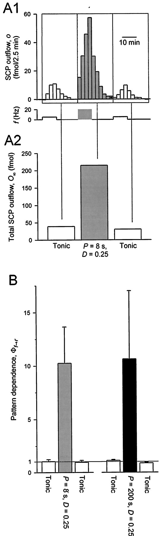
Experimental discrimination between Models I and II by test of the pattern dependence predicted in Figure 7. Specifically, the two patterns in Figure 7, A3 andB3, i.e., P = 8 sec and P = 200 sec, both with D = 0.25 and〈f〉 = 5 Hz, were compared. Color coding as in Figure 7. A, Representative experiment. A1,Time course of SCP outflow while motor neuron B15 was stimulated to fire as shown below, with the test pattern, in this case P = 8 sec (dark gray block), between two blocks of unpatterned, tonic firing at 〈f〉 = 5 Hz. Each bar of outflow is the amount of SCP contained in each 2.5 min drop of ARC perfusate (see Release experiments in Materials and Methods).A2, Total SCP outflow, O∞ , resulting from each block of patterned or unpatterned firing, obtained by summing the indicated bars of A1. B, Group data. Means ± SEM of plots like A2 from four experiments with each test pattern. In each experiment, the plot was first normalized by the mean of the two blocks of unpatterned outflow so as to yield, for the two test patterns, directly the pattern dependence Φf→r.
Viewed another way, Equation 21 states that, in general, the mean amplitude of the output X depends both on the mean amplitude of the input f and on its pattern, as described by Φf→X.
Φf→X is determined by interaction of the pattern of f with the nonlinearity of the f → X transformation. Φf→X = 1 (no pattern dependence) when, at one extreme, f is unpatterned (f → X can then be any function) or, at the other extreme, when f → X is a linear transformation (f can then have any pattern). Otherwise, when both pattern and nonlinearity are present, Φf→X ≠ 1: there is pattern dependence, of a type determined by the shape of the nonlinearity (see below).
The key point is that, in general, both the pattern and the nonlinearity have associated time scales on which they are expressed. Thus, here f(t) is only patterned on time scales shorter than the cycle period P, whereas the nonlinearity of, for instance, the slow reaction f → px becomes expressed on time scales longer than the relaxation time τpx. Only if the time scales overlap, so that the pattern and the nonlinearity are able to interact, does pattern dependence become expressed.
Pattern dependence generated by Models I and II
We now use this framework to explain the pattern dependence generated by Models I and II, first by their slow and fast reactions separately (Fig. 6), then overall (Fig. 7).
In Figure 6, in each of the four parts A1–B2, we have plotted the pattern dependence generated by each of the four reactions for firing patterns over a wide range of cycle period P and duty cycle D (note that log scales are used), all at the same mean firing frequency 〈f〉. (Strictly, the plots are specific for this value of 〈f〉, but plots for other 〈f〉 are similar.) Two examples of the actual waveforms are shown at the top left and top right of each of A1–B2, in each case comparing, as Equation 21 does, the patterned waveform f(t) and the steady-state output waveform that it produces (thick traces) with the unpatterned, tonic firing at 〈f〉 and its output (thin lines). The properties of the pattern dependence can then be correlated with the shape of the steady-state transformation produced by the reaction, in the top centerof each of A1–B2.
Fast reaction, Model I
We start with the simplest case. In Model I, the fast reaction, f → r, fast (Fig. 6A2), is linear. Therefore it cannot generate pattern dependence with any pattern; for all patterns, Φf→r,fast,Model I = 1. The mean output 〈r〉 is the same, through this reaction, no matter what temporal pattern the motor neuron spikes are arranged in.
Slow reaction, Model II
The slow reaction of Model II, f → p (Fig.6A2), is, for small, physiological values of p, also essentially linear. Thus it cannot generate pattern dependence either. Unlike the previous reaction, this reaction is not instantaneous: its output p(t) hardly responds at all to fast patterns with cycle periods P < τp; it responds only to slow patterns with P ≥ τp (Figs. 5A, 6A2, top left andtop right). Nevertheless, Φf→p,Model II ≈ 1 for all patterns, whether fast or slow.
Fast reaction, Model II
The fast reaction, f → r, fast, of Model II (Fig.6B2) is supralinear. This shape of nonlinearity generates “positive” pattern dependence, Φf→r,fast,Model II > 1 (Brezina et al., 1997): the mean output 〈r〉 is greater when the spikes are grouped into bursts than when they are dispersed in tonic firing. Pattern dependence progressively increases as the bursts become more extreme, as the duty cycle D decreases from D = 1 along the right front edge of the main plot of Figure 6B2 (unpatterned, tonic firing, for which, by definition, Φ = 1) toward left rear. Although nonlinear, the reaction is instantaneous so that the nonlinearity overlaps and interacts with patterns on all time scales, equally with all cycle periods P. Thus the pattern dependence does not vary with P. Indeed, Equation 13 in Materials and Methods shows that, simply, Φf→r,fast,Model II = D1−y =1/D2 with y = 3.
Slow reaction, Model I
Finally, the most complex case, the slow reaction of Model I, f → p4 (Fig. 6A1), is nonlinear, but also noninstantaneous. It hardly responds at all to fast patterns with cycle periods P < τp4; it responds only to slow patterns with P ≥ τp4 (Fig.6A1, top left and top right). For the former, the reaction becomes effectively linear (Brezina et al., 1997) and so, for P < τp4, Φf→p4,Model I≈ 1 (flat region at the left-hand end of the main plot of Fig.6A1). The nonlinearity of the reaction, and so the pattern dependence that it generates, is expressed only for patterns with P ≥ τp4. The nonlinearity is sigmoidal: supralinear for small, physiological p4 but sublinear (saturating) for large p4. There is therefore primarily positive pattern dependence (Φf→p4,Model I> 1), but at very large P and very small D (in the right rear corner of the main plot of Fig. 6A1), where p4 becomes large, this is diminished again by the opposite, “negative” pattern dependence generated by the sublinearity (Brezina et al., 1997).
Overall pattern dependence
How the pattern dependence generated by the individual slow and fast reactions then combines to give the overall pattern dependence of release, Φf→r, generated by Models I and II is shown in Figure 7, A1 and B1 (over a wide range of P and D, on log scales), and A2 and B2 (for a more physiological subset of the patterns, on linear scales).
As Equation 19 implies, the pattern dependence of the two reactions, in the first instance, simply multiplies to give the overall pattern dependence. In Model I, Φf→r,fast = 1, and so the overall pattern dependence Φf→r reflects in the first instance just the pattern dependence of the slow reaction, Φf→p4. In Model II, conversely, Φf→p ≈ 1, and so the overall Φf→r reflects in the first instance just the pattern dependence of the fast reaction, Φf→r,fast. However, when the output of both individual reactions is itself patterned, in a temporally correlated way because the same input pattern of f(t) has penetrated into both, an additional component of the overall pattern dependence arises from this correlation. This is not the case for patterns with P < τpx, which do not penetrate through the slow reaction to its output, p(t)x, which is essentially constant. WhenP ≥ τpx, however, both individual reactions produce patterned output that is temporally correlated—simultaneously high when f(t) = fintra, and simultaneously low when f(t) = 0 —in effect adding supralinearity to the overall transformation and so making the overall Φf→r even more positive (compare Fig. 6A1 with 7A1 and 6B2 with 7B1). Ultimately, when P ≫ τpx, Equation 20 yields the real relation r(t) ∝ f(t)xf(t)y = f(t)x+y [for small f(t)]. For Model II, for instance, this gives (by Eq. 13) Φf→r = 1/D3 as compared with Φf→r,fast = 1/D2, a steeper growth of positive pattern dependence with decreasing D, visible at the right-hand end of Figure 7B1.
Thus, as comparison of Figure 7, A and B, shows, Models I and II predict very different pattern dependence of release. Model II predicts positive pattern dependence on all time scales, for firing patterns with all cycle periods P, whereas Model I predicts positive pattern dependence only for slow patterns. For fast patterns, those with P < τp4, it predicts pattern-independent release.
Experimental test of the pattern dependence predicted by Models I and II
In their experiments, Vilim et al. (1996a,b) used firing patterns with cycle periods P ranging from 5 to 10.5 sec and duty cycles D ranging from 0.5 to 0.3. This range of patterns is indicated by the dark gray region labeledVilim in Figure 7, A2 and B2. Within this range, no effect of pattern release could be resolved; release appeared to vary simply with the mean firing frequency 〈f〉 (Vilim et al., 1996b). In other words, release over this range appeared to have the samerelative pattern dependence. This is consistent with the predictions of Model I.
This range of patterns, however, is very narrow, and, in particular, does not include D = 1, that is, the comparison with unpatterned, tonic firing needed to establish the absolutepattern dependence as defined by Equation 21. We therefore performed a series of experiments, similar to those of Vilim et al. (1996a,b), to establish the absolute pattern dependence, and more generally to discriminate between Models I and II on the basis of their predicted pattern dependence.
As best suited for this purpose, we selected two particular test patterns, P = 8 sec and P = 200 sec, both with D = 0.25 and 〈f〉 = 5 Hz [the first of these is similar to the patterns used byVilim et al. (1996a,b); note that it is much faster than the temporal resolution of the release measurements], in addition to the tonic firing at 〈f〉 = 5 Hz. In Figures 7and 8, these are color-coded dark gray, black, and white, respectively. For each of the two test patterns, we measured the absolute pattern dependence of release in the way illustrated in Figure 8A.
The predictions of Models I and II for these two patterns are contrasted in Figure 7, A3 and B3. Model I predicts essentially pattern-independent release for the fast pattern, P = 8 sec, and modest positive pattern dependence for the slow pattern, P = 200 sec. In contrast, Model II predicts similar, and much larger, positive pattern dependence for both patterns.
The experimental data are summarized in Figure 8B. With both patterns, there was similar, and very substantial, positive pattern dependence: ∼10-fold greater release with each pattern than with the same number of spikes presented unpatterned. Clearly, the real release resembles the predictions of Model II, and not at all those of Model I. Model I must be rejected, and Model II is to be preferred as a description of the release of peptides from motor neuron B15.
Looking back at the data of Vilim et al. (1996a,b), we see that Model I predicts no difference in release for the patterns used there only by making the release produced by all of themabsolutely pattern independent, with Φf→r = 1. This is clearly contradicted by the new data. Model II well explains the new data, but it does predict some variation in release over the range of patterns ofVilim et al. (1996a,b) (Fig. 7B2). Over the narrow range used, however, the largest difference is only approximately twofold, which might simply not have been resolved against the inherently large variability of release in this preparation (see magnitude of error bars in Fig. 8B).
The results in Figure 8 bear out the conclusions of Whim and Lloyd, who, although with less direct methods of monitoring release (Whim and Lloyd, 1989, 1990) or working in tissue culture rather than the intact system (Whim and Lloyd, 1994), examined a broad range of patterns, including D = 1, and reported substantial pattern dependence of peptide release from motor neuron B15.
DISCUSSION
In this paper we have constructed, on the basis of existing experimental data, a mathematical model of release of the peptide transmitters, the SCPs and BUCs, from motor neuron B15 in the ARC neuromuscular system of Aplysia. Experimentally, however, it was possible to measure only the mean, heavily averaged release. The minimal model is therefore very simple. It consists of a slow “mobilizing” or “facilitating” reaction (see further below) and the fast release reaction itself. The former is slow enough to be directly observable in the data. The latter is not; we have simply lumped together all fast components of release, inferred to exist from indirect evidence, into one instantaneous reaction. Altogether, release is instantaneously gated by the firing pattern, but its envelope waxes and wanes slowly in response to changes in the mean firing frequency, and very slowly declines as the releasable pool of peptide becomes depleted (Fig. 5).
However, when used in the conventional way—by examining the time course of the waveform of release elicited by each individual firing pattern—the data did not have the temporal resolution to completely specify the details of even this simple model. In particular, the observed release increases highly supralinearly with firing frequency, and this supralinearity could equally well be attributed to the slow reaction (Model I) or to the unobservable fast reaction (Model II) (or, in reality, probably in some ratio to both). We were able, however, to discriminate between Models I and II by using the mean-release data in a different, more global way, by considering its pattern dependence.
Temporal pattern dependence as probe of the release process
In general, mean release depends not only on the “amount” of stimulation—here, the number of motor neuron spikes—but also on its temporal pattern. As we illustrated with our two models in Figures 6and 7, this pattern dependence arises from, and its type and magnitude are governed by, interaction of the pattern with the nonlinearities of the release reactions, which in turn depends on overlap of their respective time scales (Brezina et al., 1997). Reactions with different nonlinearities and kinetics thus generate different pattern dependence for a particular pattern, and different global surfaces of pattern dependence, such as we plotted in Figures 6 and 7, over a range of patterns. Here, attributing the supralinearity to the slow or the fast reaction in Models I and II predicted, respectively, pattern-independent or substantially pattern-dependent release for fast patterns, those faster than the relaxation time of the slow reaction but not of the fast reaction. Our experiments confirmed the latter prediction, that of Model II.
Conversely, an experimental mapping of the surface of pattern dependence could guide subsequent modeling. A surface of positive pattern dependence extending to fast patterns, as in Figure7B1, would immediately suggest supralinearity residing in a fast reaction, whereas decline of the pattern dependence for patterns faster than a certain speed, as in Figure 7A1, would suggest a reaction with that characteristic relaxation time. A pattern-independent surface would imply a linear reaction.
In essence, when low temporal resolution precludes observation of the detailed waveform of release, but yields only a single number, the mean release, for each pattern of stimulation, we can compensate by systematically correlating this number over a range of patterns. By applying patterns faster than the resolution of the release measurements, we can probe even fast, directly unobservable processes of release.
Relation to cellular release processes studied in other systems
How does our model and its predicted pattern dependence relate to what has been found, in much more concrete cellular detail, in preparations in which release, as well as intracellular Ca2+, has been measured with high temporal resolution?
It will be important to recall that release of transmitters and hormones ranges from “fast” (release of classical fast neurotransmitters from SSVs) to “slow” (release or secretion of slower-acting neuropeptides and hormones from LDCVs or secretory granules) (Martin, 1994; Verhage et al., 1994; Morgan and Burgoyne, 1997; Kasai, 1999). Indeed, motor neuron B15 itself is a mixed fast/slow system, performing not only the slow peptide release that we have studied here but also, from the same terminals, fast release of ACh.
In both fast and slow release, activity-dependent elevation of the intracellular Ca2+ concentration ([Ca2+]i) not only triggers the release on a fast time scale but also, on slower time scales, augments it through Ca2+-dependent modulatory reactions. Physically, these may involve mobilization of vesicles from distal to more proximal pools in the release pathway (Neher and Zucker, 1993; Thomas et al., 1993; von Rüden and Neher, 1993; Horrigan and Bookman, 1994; Gillis and Chow, 1997; Neher, 1998; Gomis et al., 1999); functionally, they appear as the multiple components of facilitation and potentiation of release that are well known, in particular, at fast synapses (Zucker, 1989, 1996;Fisher et al., 1997).
These slow Ca2+-dependent preparatory or modulatory reactions, and the final fast Ca2+-dependent release, respectively, provide a natural interpretation for the firing frequency-dependent slow and fast reactions in our model. Our model is consistent, for instance, with that of Heinemann et al. (1993):
 Equation 22Our equations, however, are somewhat simplified from those describing the full model in Equation 22. In particular, the release-ready pool does not have an autonomous existence in our model; release is, in effect, always rate-limited by the slow mobilizing reaction. This indeed may be the rule in slow systems with prolonged stimulation (Neher and Zucker, 1993; Martin, 1994; Gillis and Chow, 1997). At rest, the release-ready pool is empty in our model. Again, this fits with the observation that LDCVs and secretory granules, in contrast to SSVs, are mostly not predocked at release sites (Burke et al., 1997; Morgan and Burgoyne, 1997). The resulting pattern of a slow build-up of release from zero after stimulation starts (Fig. 5C) is commonly seen in slow systems (Ämmälä et al., 1993; Seward et al., 1995; Seward and Nowycky, 1996).
In our preferred Model II, the slow reaction is linear, and the fast reaction supralinear. This fits well what is known about the corresponding real reactions. In addition, it highlights a significant difference between fast and slow release and its pattern dependence.
In fast systems, the final release is controlled by a sensor that binds and unbinds Ca2+ rapidly but with very low affinity (>100 μm), in response to high but brief and localized elevations of [Ca2+]i centered on the inner mouths of open Ca channels (Smith and Augustine, 1988; Heidelberger et al., 1994; Zucker, 1996; Neher, 1998; Kasai, 1999). The intrinsic [Ca2+]i-release relation is highly supralinear (Augustine et al., 1987;Heidelberger et al., 1994; Zucker, 1996). However, this supralinearity will not be evident. Because the relevant [Ca2+]i elevation and reaction of the sensor are much faster than the inter-spike interval, each spike will trigger release in a discrete, stereotyped, independent manner. Total release will reflect simply the number of spikes, regardless of their arrangement—it will be linearly dependent on the firing frequency, and pattern independent. Indeed, ACh release from motor neuron B15 increases relatively linearly with firing frequency (Lloyd and Church, 1994).
In slow systems, in contrast, the final release is controlled by a higher-affinity sensor responding to [Ca2+]i elevations that are less high (perhaps only 10 μm), less brief, and less localized (Ämmälä et al., 1993; Thomas et al., 1993; Burgoyne and Morgan, 1995). This is closely connected with the fact that slow release is loosely coupled, spatially and therefore also temporally, to Ca2+entry (Verhage et al., 1994; Chow et al., 1996; Morgan and Burgoyne, 1997;Mansvelder and Kits, 1998). Under these circumstances, [Ca2+]i can integrate with repeated spikes to a level where a significant proportion of the sensor sites are occupied. The fact that here, too, the [Ca2+]i-release relation is highly supralinear (Heinemann et al., 1993; Thomas et al., 1993) will then become significant and generate positive pattern dependence. This is a possible cellular interpretation of the pattern dependence generated by our Model II. It is, in fact, the “residual Ca2+ hypothesis” of synaptic facilitation in its original formulation (Zucker, 1989,1996).
With distance from the Ca channels and after they close, the high [Ca2+]i rapidly dissipates to leave a low (<1 μm), spatially uniform, and long-lasting [Ca2+]i elevation, believed to mediate the slow Ca2+-dependent reactions (Swandulla et al., 1991; von Rüden and Neher, 1993;Delaney and Tank, 1994; Kamiya and Zucker, 1994; Regehr et al., 1994; Burgoyne and Morgan, 1995; Zucker, 1996; Fisher et al., 1997). These reactions typically depend relatively linearly on the residual [Ca2+]i, which in turn depends relatively linearly on the firing frequency (Peng and Zucker, 1993; Regehr et al., 1994). These processes will generate relatively little pattern dependence.
Overall, both in our model and in reality, the peptide release from motor neuron B15 shows positive pattern dependence—it is greater when spikes are grouped into bursts. This is typical of peptide and other slow release (Dutton and Dyball, 1979; Andersson et al., 1982; Ip and Zigmond, 1984;Cazalis et al., 1985; Bicknell, 1988;Peng and Horn, 1991), with important physiological consequences (Gillies, 1997; Leng and Brown, 1997).
It is usually said that this behavior is caused by a slow process that “integrates” the spikes. As we have seen, some integration is necessary simply to detect the spike pattern. But more importantly, the release process must be supralinear. A linear or sublinear process may also slowly integrate, but it will generate no pattern dependence or indeed the opposite, negative pattern dependence (Fig. 6B1). Differences in this respect between fast and slow release, as well as the generally different time scales of the nonlinearities (Fisher et al., 1997), imply differences in pattern dependence in the two cases. The two kinds of release will thus be differentially elicited by various firing patterns, allowing mixed fast/slow synapses, such as those of motor neuron B15, to act as two differentially controllable channels of communication with different but complementary functions (Vilim et al., 1996b).
Footnotes
This work was funded by National Institutes of Health Grants MH36730 and K05 MH01427 to K.R.W. We thank F. S. Vilim for providing raw experimental data.
Correspondence should be addressed to Dr. Vladimir Brezina, Department of Physiology and Biophysics, Box 1218, Mount Sinai School of Medicine, One Gustave L. Levy Place, New York, NY 10029. E-mailVladimir.Brezina{at}mssm.edu.


