

Abstract
When the flat faces of a coin are grasped between thumb and index finger, a “curved edge” is felt. Analogous curved edges were generated by our stimuli, which comprised the flat face of segments of annuli applied passively to immobilized fingers. Humans could scale the curvature of the annulus and could discriminate changes in curvature of ∼20 m−1. The responses of single slowly adapting type I afferents (SAIs) recorded in anesthetized monkeys could be quantified by the product of two factors: their sensitivity and a spatial profile dependent only on the radius of the annulus. This allowed us to reconstruct realistic SAI population responses that included noise, variation in fiber sensitivity, and varying innervation patterns. The critical question was how relatively small populations (∼70 active fibers) can encode edge curvature with such precision. A template-matching approach was used to establish the accuracy of edge representation in the population. The known large interfiber variability in sensitivity had no effect on curvature resolution. Neural resolution was superior to human performance until large levels of central noise were present showing that, unlike simple detection, spatial processing is limited centrally. In contrast to the behavior of mean response codes, neural resolution improved with increasing covariance in noise. Surprisingly, resolution for any single population varied considerably with small changes in the position of the stimulus relative to the SAI matrix. Overall innervation density was not as critical as the spacing of receptive fields at right angles to the edge.
- tactile resolution
- mechanoreceptive afferents
- somatosensory
- form processing
- spatial coding
- innervation density
- curvature
- edges
It has been recognized for a long time that edges are an important feature of tactile stimuli. Information about these features is relayed to the CNS principally by the slowly adapting type I afferents (SAIs) that are highly sensitive to edges (Vierck, 1979; Phillips and Johnson, 1981a; Johansson et al., 1982). The reason for this sensitivity is that SAIs respond to strain energy density or its equivalent (Phillips and Johnson, 1981b;Srinivasan and Dandekar, 1996); therefore they are also very responsive to rectilinear corners (Blake et al., 1997b) and to circular punctate stimuli with small diameters (Mountcastle et al., 1966). Studies to date have characterized human psychophysical performance and SAI responses only for edges that are straight and relatively long (Phillips and Johnson, 1981a). However, the edges of many important tactile stimuli are not straight, but are curved. This situation is exemplified by tasks such as grasping the flat surfaces of a coin between the thumb and index finger. The stimulus is the curved edge of a surface that is flat in the plane of the skin; this is in marked contrast to grasping a sphere, where the curvature is at right angles to the skin surface. When identifying or manipulating objects such as the grasped coin, it is not sufficient to know that an edge is present; the shape (curvature) of the edge and its position on the skin must be signaled to the CNS. There is no information available about the precision with which humans can discriminate such curved edges.
Currently it is not known how the edge sensitivity of cutaneous mechanoreceptors changes with the curvature of an edge, but it is obvious that enhanced mechanoreceptor responses cannot, in themselves, provide information about the shape of an edge. Such information can only be conveyed by distributed spatial signals within a population of afferents (Doetsch, 2000). Tactile spatial coding has been analyzed for a variety of stimuli, including three-dimensional objects of various shapes (LaMotte and Srinivasan, 1987, 1996; Goodwin et al., 1995;Dodson et al., 1998; LaMotte et al., 1998) and patterns of raised dots and letters (Phillips et al., 1990; Connor and Johnson, 1992; Johnson et al., 1995). Understanding how curved edges could be encoded presents a particular challenge because the number of afferents activated will be relatively small compared with the spatial precision required (Johansson and Vallbo, 1979; Darian-Smith and Kenins, 1980). Thus, it might be expected that parameters of the afferent population, such as innervation density, could have a profound effect on resolution. Because it is not currently possible to record from the entire population simultaneously, such issues can only be addressed by simulating population responses.
In this study we quantified the human capacity to scale and discriminate the curved edges of flat stimuli. We then recorded from single primary afferent fibers and used the data to reconstruct realistic SAI population responses, which were then compared with the human performance. By varying the population parameters (individual afferent sensitivities, pattern and density of innervation, neural noise, and correlation) we elucidated the neural mechanisms underlying this type of form processing in the tactile system.
MATERIALS AND METHODS
The stimuli consisted of a series of annular segments of Delrin, 1.5-mm-wide, with curvatures ranging from 107 m−1 (radius of curvature 9.3 mm) to a straight segment, curvature 0 m−1 (radius of curvature ∞) (Fig.1A,B). For all but the largest curvatures, 107 and 84.7 m−1(smallest radii), the length of the chord b through the end points of each segment was 25 mm. This ensured that the ends of the segments did not contact the fingerpad. The stimuli were fixed ata to a hub attached to a gravity operated, balanced-beam stimulator described previously (Goodwin et al., 1991) that lowered a selected stimulus onto the fingerpad (dark line c highlights the surface that made skin contact). Contact force was set by a counterbalance weight on the beam and calibrated to a resolution of 0.1 gram force (gf). A rotary damper controlled vertical motion of the beam so that the surface of the stimulus contacted the skin at a velocity of ∼20 mm/sec. The beam was mounted on an x–y stage fitted with micrometers and dial indicators; this enabled stimuli to be positioned with a resolution of 0.01 mm. The stimuli were applied passively to the fingerpad and were orientated orthogonal to the axis of the finger with the concave side distal (Fig. 1C).

Stimulus dimensions and conventions.A, The stimuli, annular segments of Delrin 1.5-mm-wide, were fixed by post a to a hub attached to a gravity-operated, balanced-beam stimulator. The superimposed dark line c indicates the stimulus surface that made contact with the skin. The chord b was 25-mm-long for all stimuli, except curvatures 107 and 84.7 m−1 where it was 20 mm.B, The six stimuli used in the human scaling and the neural experiments. Roman numerals I andII identify the two standard stimuli used in the human discrimination experiments, 25.6 and 61.7 m−1, respectively. C, In monkey neural experiments the origin of the x–y coordinate system was located at the receptive field center (rfc), and the center of the surface (e) was positioned at different points on the skin. The center of the circle of curvature is shown byo, and d is the shortest distance from the rfc to the circle. The circle forms the midline of the annular segment, i.e., 0.75 mm from both edges. D,In population reconstructions the origin of thex′–y′ coordinate system was located at the center of the annular segment (e), and different fibers in the population had receptive field centers (rfc) located at different points on the skin.
Human psychophysics
Human capacity to perceive the curvature of an annular segment was measured in two ways; first in a series of scaling experiments and then in a series of discrimination experiments. The same six subjects (five females, one male) ranging in age from 20 to 25 years, took part in both of these experiments. The subject was seated comfortably with forearm supinated and the index finger of the dominant hand secured in a plasticine finger mold to prevent lateral movement between stimulus and finger; a curtain prevented the subject from seeing either the stimulator or their finger. The stimulus in each experiment was applied to the distal portion of the fingerpad at a contact force of 0.49 N (50 gf). Between trials, the position of the stimulus was varied randomly along the long axis of the finger to ensure that subjects were using information about the shape of the stimuli and not any spurious cues. The range of random position variation was ±1 mm from the initial contact point.
Each subject underwent an extensive training period, during which performance improved, so that by the time data were collected, the subject's performance had stabilized at the optimum level.
Curvature scaling. Six stimuli with different curvatures, 0–107 m−1 (Fig.1B), were presented in random order in blocks of 30 trials; each trial consisted of the presentation of a single stimulus for 1 sec with 3 sec between trials and a 2 min rest break between blocks. A reference stimulus, which had a mid-range curvature of 61.7 m−1, was presented a number of times at the commencement of each block and after every 10 trials within each block. To establish some consistency in scale, subjects were asked to assign this reference stimulus an arbitrary value of 50 and to estimate the magnitude of the curvature of all stimuli relative to this, e.g., if they perceived a test stimulus as being twice as curved as the reference stimulus, they were instructed to assign it a value double that of the reference. Eight such blocks were presented so thatn = 40 for each stimulus for each subject. The order of stimulus presentation was varied randomly within and between blocks.
Curvature discrimination. A two-alternative forced-choice paradigm was used to measure the subject's ability to discriminate small differences in the curvature of annular segments. Stimuli were presented in pairs: the standard, for 1 sec, followed by the comparison, for 1 sec, with an interval of ∼2 sec between them. Two stimulus conditions were used: in one (Ss) the curvature of the comparison stimulus was the same as that of the standard, and in the other condition (Sd), the curvature of the comparison stimulus was greater (smaller radius) than that of the standard. Subjects were required to judge whether the two stimuli in the pair were the same (Rs) or different (Rd). Two standard stimuli were used: curvatures 25.6 and 61.7 m−1(Fig. 1B). The curvatures of the comparison stimuli were 31, 41.2, and 61.7 m−1 for the less curved standard and 70.2, 84.7, and 107 m−1 for the more curved standard. The range of comparison curvatures was chosen to provide values below and above the likely difference thresholds. In each experimental session, six blocks of trials were presented, three for each standard (using the corresponding three comparison stimuli); each block consisted of 20 trials, 10 of which were Ss and 10Sd, presented in random order. The order of presentation within and across blocks of trials was varied randomly from session to session for all subjects. After an initial training period, data were collected over five sessions (n = 300 per standard per subject). From the conditional probabilitiesp(Rd/Sd) andp(Rd/Ss), the bias-free measure of discrimination d′ was calculated (Johnson, 1980), and difference limens were determined by linear interpolation of those values for each subject.
Neural recording
Single mechanoreceptive fiber recordings were performed on twoMacaca nemestrina monkeys weighing 2.5 and 4.5 kg, respectively. All experimental procedures were approved by the University of Melbourne Ethics Committee and conformed to the National Health and Medical Research Council of Australia's Code of Practice for nonhuman primate research. An intramuscular dose of ketamine hydrochloride (15 mg/kg) plus atropine sulfate (60 μg/kg) was given before the induction of surgical anesthesia by intravenous administration of sodium pentobarbitone (15 mg/kg). An endotracheal tube was inserted (after the application of topical xylocaine spray) to maintain a patent airway and to enable continuous measurement of end-tidal carbon dioxide levels. Anesthesia was monitored throughout the experiment and maintained with titrated doses of sodium pentabarbitone. This was delivered in isotonic saline (dilution 12 mg/ml) via an intraperitoneal catheter together with additional saline to maintain hydration. Respiration rate, end-tidal carbon dioxide level, blood pressure, core temperature, heart rate, and oxygen saturation levels were monitored throughout the experiment. Body temperature was maintained at 37°C by a heat pad and insulating blankets. Antibiotic cover was provided throughout the experiment by intramuscular administration of amoxicillin (18 mg/kg) and at the end of the experiment by a single dose of procaine penicillin (60 mg/kg).
Using aseptic surgical techniques, single fibers were isolated by microdissection after exposing the median nerve first in the upper arm and then in the lower arm. The process was repeated in the other arm, making a total of four experiments for each monkey. Each experiment lasted a maximum of 18 hr, and there was a rest period of at least 2 weeks between each experiment. During this rest period the monkeys were housed in large cages, together with or adjacent to other monkeys, with access to an outdoor exercise area. They were observed closely and regularly by trained personnel and at all times were found to be in good health with no evident signs of pain or distress. Buprenorphine hydrochloride (8 μg/kg) was available for pain relief but was judged to be unnecessary. At the end of the series, the monkeys were in prime condition and showed no signs of sensory or motor deficits. They were returned to the breeding colony.
The afferents principally activated by our stimuli were the SAIs. This afferent class was therefore selected for study. Fibers were classified by established response criteria (Talbot et al., 1968; Vallbo and Johansson, 1984). The most sensitive spot in the receptive field of each fiber was located using calibrated von Frey filaments; this is subsequently referred to as the receptive field center. Only those fibers with receptive field centers close to the central, relatively flat region of the fingerpad were used. This ensured that any effects caused by the curvature on the sides or end of the fingerpad or attributable to changes in skin mechanics close to the interphalangeal joint were minimized. Once the most sensitive spot had been identified, the finger was immobilized (with the most sensitive spot uppermost) in a customized mold with the fingernail glued to the mold; this was then secured to a hand holder. The finger was positioned so that when the stimulus made contact with the skin, the surface of the stimulus was tangential to the fingerpad, and the line of force was normal to that plane; contact force was set at 0.196 N (20 gf). The contact force used in the neural recording experiments is approximately equivalent to that used in the human psychophysics experiments scaled to take account of the difference in size between human and monkey fingerpads (for rationale, see Goodwin et al., 1997).
Six stimuli were used for all fibers: one stimulus was a straight segment (curvature 0 m−1, radius ∞), and the others had curvatures of 25.6, 34.2, 61.7, 84.7, and 107 m−1 (radii of curvature 39.1, 29.2, 16.2, 11.8, and 9.3 mm, respectively) (Fig. 1B). Responses were recorded from a total of 14 fibers using the following protocol. For each fiber, the origin of the x–y coordinate system was located at the receptive field center. First, the center of the segment (Fig. 1C, e) was presented at positions separated by 0.5 mm along the y-axis, starting with the most proximal position used. At each position the stimulus was applied for 1.5 sec (a single trial), and the time between successive presentations was 3 sec. This presentation sequence was performed for all six stimuli, and then the entire sequence was repeated twice (n = 3 per stimulus for each fiber); n = 3 was deemed sufficient because we and others have shown that variation in the responses of peripheral fibers is low (Edin et al., 1995; Wheat et al., 1995; Vega-Bermudez and Johnson, 1999). This entire procedure was repeated along lines parallel to the long axis of the finger and separated by 1 mm in ±xdirections. The order of the lines depended on the location of the receptive field. The order of presentation of the different curvatures was varied randomly between fibers, but for individual fibers it was maintained across all data collection lines, i.e., at all values ofx. At the commencement of each traverse of the receptive field, a lead stimulus with the same time sequence, 1.5 sec on and 3 sec off, was presented to minimize differential interaction effects. Data from this trial were not included in the analyses with the result that for each trial analyzed, the intertrial time period was constant.
RESULTS
Human psychophysics
Curvature scaling
Subjects scaled the curvature of six stimuli ranging from a straight segment (curvature 0 m−1) to one with a curvature of 107 m−1 (radius of curvature, 9.3 mm). Stimuli were presented passively to an immobilized finger, therefore the only source of information about the stimuli available to the subjects derived from cutaneous sources. An additional feature of the protocol we adopted, i.e., randomly varying the position of successive stimuli on the fingerpad, ensured that estimations about stimulus magnitude were based on information about the comparative shape of the stimuli and not on any spurious positional cues.
As stimulus curvature increased, the subjects' perception of the magnitude of curvature also increased. This is illustrated in Figure2A, which shows mean estimates for each stimulus for each subject; the thick line represents the mean across all six subjects.

Human performance. A, Scaling of segment curvature. Fine lines show perceived curvature of the six stimuli for each of the six subjects (mean curvature estimates, n = 40 for each stimulus for each subject). The thick solid line is the mean across all six subjects. B, Curvature discrimination for the 25.6 m−1 standard. Fine lines showd′ values for each of the six subjects, and thethick solid line shows mean d′ values.Filled circles show difference limens (d′ = 1.35) for each subject. C, Comparison ofd′ values (averaged across subjects;n = 6) for the two standards. Error bars show unidirectional SE.
Curvature discrimination
All subjects could scale stimulus curvature over the range 0–107 m−1. To determine the smallest difference in curvature that could be discriminated, the same six subjects took part in a series of discrimination experiments using subsets of stimuli from within this range. Two standard stimuli were used (curvature 25.6 and 61.7 m−1) to determine whether performance depended on the magnitude of stimulus curvature. Indices of discrimination d′, calculated from the conditional probabilitiesp(Rd/Sd) andp(Rd/Ss), are shown for all six subjects in Figure 2B for the 25.6 m−1 standard. The solid line shows the mean d′ values across the six subjects. The relationship between the curvature of the annular segment and discrimination performance was approximately linear. For each subject, the difference limen was estimated by linear interpolation of the two data points on either side of d′ = 1.35 (Fig. 2B,filled circles).
Performance with the more curved (61.7 m−1) standard was similar to that with the less curved standard. Difference limens for each subject are shown in Table 1 for both standards. The meand′ values across the six subjects are compared for the two standards in Figure 2C. The mean difference limens, 23.0 and 20.8 m−1 for standards of 25.6 and 61.7 m−1, respectively (Table 1) were not significantly different (p = 0.59; two-tailed paired t test; n = 6). Neither were there significant differences in performance between standards when all 18 pairs of data points (six subjects × three curvatures) were considered: there were no significant differences (p > 0.1) in either slope or elevation between performances for the two standards (Zar, 1984).
Difference limens (m−1) for discriminating the curvature of an annular segment
Neural responses
To generate receptive field profiles for single SAI fibers, stimuli were presented for 1.5 sec successively at a matrix of points on the skin; points were separated by 0.5 mm in the ydirection and 1 mm in the x direction. The x andy coordinates refer to the position of the centere of the annular segment with respect to the receptive field center (Fig. 1C). Care was taken to avoid values ofx that were large enough for the end points of the stimulus to contact the skin. The response measure used is the mean response (n = 3) evoked in the first second of stimulus contact.
Figure 3A compares responses of a typical single fiber to all six stimuli of different curvature at different positions along the y-axis. These profiles show three key features. First, all six profiles superimpose, indicating that the response of the afferent depended only on the distance of the receptive field center from the center of the stimulus and not on the curvature of the stimulus as such. Second, there are two response peaks corresponding to the two edges of the annular segment. Third, the skirts of the profiles are Gaussian in shape. In Figure 3B,profiles along a line parallel to the axis of the finger at a distance of 6 mm from the receptive field center are illustrated for four of the stimuli. As the curvature of the segment increases, the profiles shift to the left of the figure. Also, with increasing curvature the profiles become broader and increasingly asymmetric; it is clear that at a curvature of 107 m−1 (thick broken line) the skirt on the right side (increasing y) is steeper than the skirt on the left side (decreasing y). In Figure3C, profiles for one stimulus, curvature 84.7 m−1, are shown along a number of lines, parallel to the finger axis, at increasing distances from the receptive field center. With increasing values of x, the profiles shift to the left and become broader and increasingly asymmetric with a steeper skirt on the right; compare profile at x = 0 (solid line) with that at x = 6 mm (thick broken line). For all afferents, responses were highly consistent among the three repetitions in keeping with previous observations on the low variability of peripheral neural responses. A second order effect can be seen in Figure 3A; the asymmetry of the two peaks increases with increasing curvature.

Responses of a single fiber to stimuli of different curvature at different positions in the receptive field. Thex and y coordinates define the position of the center of the annular segment with respect to the afferent's receptive field center. Responses are the number of impulses occurring in the first second of stimulus contact. A, The six profiles show the mean responses (n = 3) to each of the six stimuli along the y-axis (x= 0). B, Mean responses elicited along a line (parallel to the y-axis) at x = 6 mm for four of the stimuli. For clarity, only one representative bidirectional SD is shown for each of two profiles (n = 3).C, Mean responses for one stimulus, curvature 84.7 m−1, along lines parallel to they-axis.
All fibers responded with similarly shaped profiles, but the magnitudes of the responses varied widely, indicating a wide spread in fiber sensitivity. To reveal the underlying response characteristics common to all fibers in our sample (n = 14) in the absence of sensitivity differences, we normalized the responses of each fiber. This was done by dividing the responses of each fiber by the average response of that fiber to the straight stimulus over seven data points along the y-axis spanning the center of the receptive field; this region corresponded across all fibers. Consistent with our previous studies, the normalizing factors were normally distributed with a coefficient of variation of 0.35 (Goodwin et al., 1995; Wheat and Goodwin, 2000). When the normalized responses were pooled, it was clear that all fibers in the sample produced similarly shaped profiles. This is exemplified in Figure4A, which shows mean normalized responses of the 14 SAI fibers to the straight stimulus (curvature 0 m−1) along they-axis. Figure 4B shows that, as with the single fiber data illustrated in Figure 3A, responses of all fibers along the y-axis were invariant with stimulus curvature; data shown in this figure are mean normalized responses of 14 fibers to each of the six stimulus curvatures (for clarity SE are shown for one stimulus only). All stimuli produced response peaks in the receptive field profiles which corresponded to the edges of the stimuli. The consistency of the profiles between fibers across the extent of the receptive field is shown in Figure 4C. These normalized profiles reflect the shape of the annular segments as is clearly evident in a representative contour plot of the two-dimensional profiles (Fig. 4D). The normalized data verify an important principle that is essential for the population reconstructions that follow. All 14 SAI responses to an annular segment can be quantified by the product of two factors. The first factor is the sensitivity of the fiber, and the second factor is the normalized profile, which is independent of the fiber sensitivity.

Normalized responses for the 14 SAIs.A, Normalized responses of each of the 14 fibers to the straight stimulus (curvature 0 m−1) atx = 0. B, Mean normalized responses (n = 14) to each of the six stimuli atx = 0; ±SE for one representative profile only.C, Mean normalized responses (n = 14) to one of the most curved stimuli (curvature 84.7 m−1) along lines at four locations along thex-axis; ±SE at two representative points.D, Contour plot of mean normalized responses (n = 14) for curvature 84.7 m−1; isometric lines are separated by increments of 0.12 (black = 0; white = 1.2).
Mathematical characterization of response profiles
The normalized receptive field profiles were similar for all fibers in the sample and could therefore be described by a single mathematical function. The data in Figures 3 and 4 suggest that the profiles conform well to the sum of two offset Gaussians (in effect one for each edge of the segment) and that the only positional variable is the radial distance from the receptive field center to the segment (Fig. 1C, d). Thus, the function used was:
 Equation 1where NR is the normalized response, and a,b, and c are the constants of the Gaussians. For an annular segment of radius r the distance d is determined by the x and y coordinates of the stimulus from the relationship, d =
 − r. Thus:
 Equation 2The constants a, b, and cwere determined by nonlinear regression using the data from all 14 afferents, for all six stimuli, at all tested locations in the receptive field: 5239 data points. These data points are plotted in Figure 5A as normalized response versus distance d, together with the regression function. The six regression constants are given in Table2. The close correspondence between the mean normalized data and the fitted function is illustrated for a representative range of curvatures and positions in Figure5B–D. The correspondence along the y-axis is shown for one of the most curved stimuli, 84.7 m−1 (Fig. 5B) and for the straight stimulus 0 m−1 (Fig.5C). Figure 5D shows the fit for the stimulus with curvature 84.7 m−1 along a line 6 mm from the receptive field center. Naturally, the function matches the changes in profile position, width, and asymmetry seen in the data.

Comparison between normalized data and the best fitting function from Equations 1 and 2. A, Data points (n = 5239) show normalized responses from 14 SAIs, for all six stimuli, at all x and ycoordinates tested, plotted as a function of the distanced in Equation 1. The solid line is the regression function. Note that because n is so large, many data points are hidden because they overlap, particularly close to the regression function. B, Responses to one of the most curved stimuli (curvature 84.7 m−1) atx = 0. C, Responses to the straight stimulus (0 m−1) at x = 0.D, Responses to the stimulus with curvature 84.7 m−1 along a line 6 mm from the center of the receptive field. B–D, Solid lines show mean normalized responses (n = 14; ±SE at representative locations), and dashed lines show the fitted function.
Simulated SAI populations
The critical issue in this series of experiments is the precision with which the neural population can reflect the essential features of the stimuli. In the following sections we explore this by simulating realistic SAI population responses. These reconstructions take into account population parameters that are not evident in single fiber responses. Fundamental parameters which degrade the representation of the stimulus in the population response are (1) the variation in sensitivity between fibers, (2) random variation in the responses of individual afferents, and (3) the sampling density and geometry.
The conventions for the simulation are shown in Figure1D. The receptive field center (rfc) of afferents in the population are specified by their x′ andy′ coordinates with the origin located at the center of the annular segment. Initially the matrix of receptive field centers (x′ij,y′ij) is uniform with a spacing of 1.2 mm, which corresponds to the estimated innervation density of 0.7 mm−2 for human fingerpad skin (Johansson and Vallbo, 1979). The total area spanned by the fibers is 12 × 12 mm, which is equivalent to the size of the central part of the average human fingertip.
The normalized response of an afferent with a receptive field center at (x′ij,y′ij) obeys Equation 2. Note thatx′ij = −xij andy′ij = −yij; for example if the coordinates of e in Figure 1C are (4, 4) then the coordinates of rfc in Figure 1D are (−4, −4), and these two figures are equivalent. As a result, population responses are mirror images of receptive field profiles. If the afferent at position (x′ij,y′ij) has a sensitivitysij then its responseREij (impulses elicited in the first second of contact) is given by:
 Equation 3where r is the radius of curvature of the annular segment, and a, b, and c are the constants given in Table 2. The factor εijallows for random neural noise in the processing pathway; initially εij is set to zero, and in later sections we will vary it systematically. The sensitivity sijof each fiber in the matrix varies randomly from fiber to fiber with a Gaussian distribution with a coefficient of variation of 0.387; the distribution of sensitivities was derived from our current and previous experimental data (Goodwin and Wheat, 1999).
Figure 6A (shaded area) shows a slice, parallel to the y′ axis atx′ = 4.8 mm, through a simulated ideal population response to a stimulus with a curvature of 61.7 m−1. The fibers within this ideal population had uniform sensitivity and a high innervation density. No noise was superimposed on these responses so that εij = 0. Corresponding response profiles for a selection of four more realistic populations are shown by the thin lines and symbols in Figure 6A. The constituent fibers had receptive fields that were arranged in a uniform configuration with a density of 0.7 mm−2(spacing 1.2 mm). Fiber sensitivities were randomly distributed following a Gaussian with a coefficient of variation of 0.387, and the pattern of sensitivities was different for each population. Comparison between the realistic and ideal profiles makes it abundantly clear that varying sensitivity has a dramatic distorting effect on the shape of the response profiles, even in the absence of response noise.

SAI population simulation.A, Slices through simulated response profiles for four populations of SAIs (thin lines andsymbols), each with a different sensitivity profile. Receptive field centers were uniformly spaced with a separation of 1.2 mm (density 0.7 mm−2). For comparison, a corresponding response profile for an ideal population (shaded area) is also shown. Stimulus curvature was 61.7 m−1. Slices are taken parallel to the long axis of the finger at x′ = 4.8 mm. B, Curvature estimates κ from each of the five populations illustrated inA for the stimuli used in the human scaling experiments. Curvature (κ) was extracted from the population responses by template matching. The close correspondence between stimulus and estimated curvature is indicated by r = 0.99 for all populations. C, Distribution of curvature estimates (κ) for one representative population with a stimulus curvature of 61.7 m−1. Response variation was the sum of two random variables, one for proportional noise (variance of εij = 1.5 REij), and one for additive noise (SD of εij = 6 impulses/sec). Mean κ was 60.0 (± 5.44 SD; n = 500), and the distribution was Gaussian (shown by the thick line). The Kolmogorov–Smirnov test found no significant difference between the distribution of κ and that of the normal distribution (p = 0.65). Fiber configuration for this simulation was uniform with a spacing of 1.2 mm (density 0.7 mm−2).
Representation of curvature in the population responses
To determine the precision with which the curvature of the stimulus was represented in the simulated population responses, we adopted a template-matching approach. We determined the curvature of the annular segment that would minimize the mean square deviation of the population response from the template response by regression of the equation:
 Equation 4The regression results in a value for the two constants, ρ the radius of curvature of the matching template and λ the mean sensitivity of the afferents in the population. We will express the result in terms of the curvature of the match, κ given by 1/ρ. In the case of an ideal population response (Fig. 6A, shaded area), κ will of course be identical to the curvature of the stimulus (Fig. 6B, thick line). In realistic populations with distortions, noise and finite innervation density, κ will differ from the stimulus curvature. The advantage of this approach is that it provides a quantitative measure of the precision of representation in realistic populations without having to make assumptions about candidate neural codes. Moreover, this is likely to measure the optimal representation (see Discussion). The nonlinear regression was performed using the Levenberg–Marquardt method (Press et al., 1986).
In spite of the severe distortions in the four population responses indicated in Figure 6A, the curvatures κ extracted from the responses of each of those populations were similar (Fig.6B). More striking is the almost perfect relationship between stimulus curvature and curvature estimated from the population responses; r = 0.99 for all four populations. The stimulus curvatures used in these simulations were those used in the human scaling experiments.
Effect of response variability on resolution in the population
Although the variability of peripheral afferents is low, there is considerable noise in the ascending pathway that will reduce resolution. In our model we account for such noise by adding a random component, εij, to the response of each fiber in the population. Two broad categories of lumped noise are used. For one category, termed “proportional noise”, the level of noise is proportional to the magnitude of the response of each fiber; thus εij in Equation 3 is a normally distributed random variable with a mean of zero and a variance proportional toREij. For the second category, “additive noise”, the noise is independent of the magnitude of the afferent's response; thus, εij is a normally distributed random variable with a mean of zero and a SD that is the same for all i and j. These choices are justified in Discussion.
With a constant stimulus, variability in each fiber's response leads to variability in the whole population response and therefore to variability in estimates of curvature κ from the population response. Figure 6C shows the distribution of κ estimated 500 times with a combination of proportional noise (variance of εij = 1.5REij) plus additive noise (SD of εij = 6 impulses/sec). The distribution is Gaussian. The mean value of κ is 60.0, which is close to the stimulus curvature of 61.7 m−1, but the distribution is broad so that most estimates of curvature from the population response will differ from the stimulus curvature, leading to errors in perception. This type of distribution was found under all stimulus and noise conditions.
To quantify the effect on discrimination of the variations in curvature estimates illustrated in Figure 6C, we used a signal detection theory approach analogous to that used in our human psychophysics experiments. Stimuli were presented to the model in pairs. For 500 pairs the first and second stimuli were both the standard, and for an additional 500 pairs the first stimulus was the standard, and the second stimulus was the comparison, which had a larger curvature (smaller radius). Curvature estimates κ were extracted from the population response to each stimulus. For each pair, the second stimulus was judged to be different if κ2 − κ1 ≥ the decision boundary (defined as half the difference between the mean value of κ for the comparison stimulus and the mean value for the standard stimulus), otherwise the two stimuli were judged to be the same. From the resultant conditional probabilities, the index of discrimination d′ was calculated, and discrimination thresholds were determined by linear regression.
In Figure 7A the ability of the model to discriminate small differences in curvature, using the more curved standard from our psychophysics experiments (61.7 m−1), is illustrated for two populations with varying sensitivity profiles and one population with uniform sensitivity. Various magnitudes of proportional and additive noise were used. As expected, increasing either component of noise decreased resolution. Doubling additive noise had a greater impact on performance than doubling proportional noise. The difference limens for populations 1 and 2 are similar and, surprisingly, so are the difference limens for the population with uniform fiber sensitivity. In other words, even if the CNS compensates for varying sensitivity, there would be no improvement in performance as demonstrated by the white bars in Figure7A.

Effect of different noise components on discrimination performance of the model. A, Standard curvature 61.7 m−1. Performance of three populations: the gray and hatched columnsshow performance of two populations with different sensitivity profiles (Gaussian distribution with a coefficient of variation of 0.387), and the white columns show the performance of a population with uniform sensitivity. B, Comparison of performance between the two standards used in the psychophysics experiments, 61.7 and 25.6 m−1 (same population aspopulation 1 in A). For all populations, fibers were uniformly arranged with 1.2 mm spacing (density 0.7 mm−2). Dotted lines inA and B indicate human difference limens for standards of 61.7 and 25.6 m−1, respectively. Noise levels in both A and B were (fromleft to right) as follows: proportional noise alone with variance = 0.75 REijand 1.5 REij, additive noise alone with SD = 4 and 8 impulses/sec, and for A only, combined proportional noise (variance = 3.5REij) plus additive noise (SD = 12 impulses/sec).
For all populations tested, performance of the model was superior to human performance (indicated by the dotted line) at the moderate noise levels represented by the four leftmost sets of bars. The right column in Figure 7A shows that high levels of noise needed to be introduced before human and model performances were on a par; in this illustration proportional noise with variance = 3.5 REij plus additive noise with SD = 12 impulses/sec. Figure 7B confirms that performance of the model with the less curved standard used in the psychophysics experiments is approximately equivalent to that with the more curved standard when tested under the conditions illustrated in Figure 7A; the population used to illustrate this is population 1. The effects of the two standards on the discriminatory capacity of the model parallel their effects on psychophysical performance.
If the only noise present were that in the primary afferent fibers, where the coefficient of variation is a few percent (Wheat et al., 1995), then the precision of curvature representation in the SAI population would far exceed the performance of our subjects.
Response covariance
The analyses so far have assumed that the noise attributed in the model to individual afferents is independent of the noise on the other afferents. However, such independence is unlikely, and correlation among the variation of responses may have a significant effect on the resolution of the population. Although covariance among lumped noise represents a simplification of the real situation, it serves to highlight the major effects that covariance has on the resolution of stimulus features represented in the population response. Values for the range of covariances occurring in the tactile pathway have not been established, so we illustrate effects over a large range to demonstrate the trends (see Discussion).
In the following section, the noise components εij have been generated such that the correlation coefficient between each i, j pair is 0, 0.4, or 0.8. Five representative levels of noise are illustrated in Figure 8: proportional noise alone with variance = 0.75 REij and 1.5REij, additive noise alone with SD = 4 and 8 impulses/sec, combined proportional noise (variance = 1.5 REij) plus additive noise (SD = 4 impulses/sec).
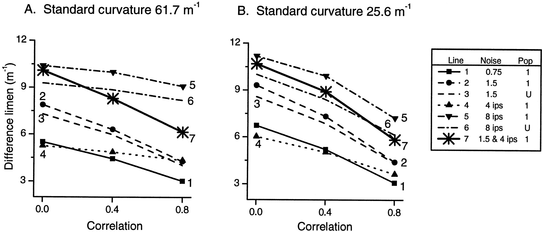
Effect of correlation on resolution in the population response for two standards: 61.7 and 25.6 m−1. Correlation coefficients for noise components εij are 0, 0.4, or 0.8 for all i,j pairs. For a realistic population with varying sensitivity (population 1), five representative levels of noise are illustrated: proportional noise alone with variance = 0.75REij (line 1) and 1.5REij, (line 2), additive noise alone with SD = 4 impulses/sec (line 4) and 8 impulses/sec (line 5), and a combination of proportional noise with variance = 1.5REij plus additive noise with SD = 4 impulses/sec (line 7). For comparison, performance of a population with uniform sensitivity (U) is shown for proportional noise with variance = 1.5 REij, (line 3) and for additive noise with SD = 8 impulses/sec (line 6).Lines with symbols indicate performance of population 1, with varying sensitivity;lines with no symbols indicate the performance of a population with uniform sensitivity.
Figure 8 illustrates that for both standards used in the psychophysics experiments, 61.7 and 25.6 m−1, resolution improved as correlation increased from 0 to 0.8. In this illustration a realistic population with varying sensitivities (population 1 described previously) was used. For the less curved standard (Fig. 8B), the trend illustrated was similar for all noise levels tested and for both types of noise (proportional and additive). For the more curved standard (Fig.8A), however, the functions for additive noise alone (lines 4, 5, and 6) were flatter than those for proportional noise alone (lines 1, 2, and 3). Maintaining uniform sensitivity across the population (lines 3 and 6) resulted in similar performance (illustrated for two levels of noise) to that of the population with varying sensitivity between fibers. Thus, even if the CNS were able to compensate for varying afferent sensitivity, little advantage in performance would be gained, as was the case when noise was uncorrelated.
Innervation density and geometry
So far we have assumed that afferents innervate the skin uniformly with a separation between receptive field centers of 1.2 mm, which corresponds to the estimated innervation density of 0.7 mm−2. However, this density is only an estimate (Johansson and Vallbo, 1979), and the real value may be considerably different. Moreover, the innervation is unlikely to be completely uniform. Given the relatively sparse innervation compared with the spatial detail that must be resolved to discriminate our stimuli, the details of innervation geometry are likely to have a considerable impact, the nature of which is not obvious a priori. In the following section we first explore the effect of varying density with a uniform pattern of innervation, and then we explore the effect of nonuniform innervation geometry.
Three uniform sampling densities were compared: the nominal density of 0.7 mm−2 (fiber spacing 1.2 mm), a higher density of 1.78 mm−2 (fiber spacing 0.75 mm), and a reduced density of 0.25 mm−2(fiber spacing 2 mm). Even for this simple comparison, there are two confounding factors. First, for more realistic populations with varying sensitivity, changing the density in a fixed area of skin also, of necessity, changes the distribution of sensitivities within the population and the distribution relative to the stimulus. To avoid this complication, we used populations with uniform sensitivity so that the effects of innervation density could be isolated. The second factor is the position of the sampling matrix relative to the stimulus, which also changes with changing density. This is demonstrated in Figure9B, which shows a slice along the y′ axis through a population response. The thin dotted lines and open circles show sampling at 3 mm intervals for one position of the fiber matrix, and the thicker broken lines and solid circles show sampling at the same density with a different position of the fiber matrix. It is obvious that, at least for this slice, the images of the stimulus “seen” by the two populations are different, although the only difference between the populations is a shift in origin. It is not possible to vary innervation density without changing the relative position of some of the afferents in the population with respect to the stimulus.

Resolution as a function of innervation density and geometry. Resolution is measured by ςκ, the SD of κ (the estimate of curvature in the population response). The standard stimulus had a curvature of 61.7 m−1.A, Distributions of ςκ for various fiber populations. In each case, the position of the population was varied randomly in both the x′ and y′ directions within a range of ±0.5 times the fiber spacing; n= 500 per population. Fiber spacing was the same in thex′ and y′ directions for distribution 1 (spacing 0.75 mm, density 1.78 mm−2), distribution 2 (spacing 1.2 mm, density 0.7 mm−2), and distribution 3 (spacing 2 mm, density 0.25 mm−2). For distributions 4 and 5, density 0.28 mm−2, spacings were 3 mm x′, 1.2 mm y′, and 1.2 mm x′, 3 mm y′, respectively.B, Indication of the effect of shifting a population relative to the stimulus. The response function being sampled is a slice, at x′ = 0, through the profile of an ideal population with infinite sampling density. The function is sampled every 3 mm by two populations with different relative locations (thin dotted lines and thick broken lines, respectively). C, Resolution indicated by the median value of ςκ. The solid black bars (marked 1–5), show the median values of the distributions (marked 1–5) in A and thus indicate the resolution of five different populations with regularly spaced receptive fields. White bars show resolution when the five populations have some scattering imposed on the receptive fields, assuming the CNS “knows” the exact positions of the fields. Hatched bars show resolution if the CNS does not know those exact positions. D, Geometric arrangement of fibers at two densities. Curved linessuperimposed over the matrices represent a stimulus with a curvature of 61.7 m−1. For density 0.25 mm−2 (top two panels), fiber configuration is either uniform and symmetrical (left) or scattered (right), in which case each fiber has been randomly shifted from the uniform configuration in the x′ and y′ directions within ±1 mm. The bottom two panels (density, 0.28 mm−2) show two alternative fiber configurations:x′ spacing 1.2 mm, y′ spacing 3 mm (left) and x′ spacing 3 mm,y′ spacing 1.2 mm (right). Responses for the analyses depicted in A and C varied randomly with a combination of proportional noise (variance of εij = 1.5 REij) plus additive noise (SD of εij = 6 impulses/sec).
To address this second factor, we varied the origin of the fiber matrix randomly in the x′ and y′ directions within the range ±0.5 times the fiber spacing. Using this approach, we created 500 populations that all had the same density, but each had a different offset with respect to the stimulus. For each of these populations, the model estimated the resolution of the representation of stimulus curvature in the population. We illustrate the results for a stimulus with a curvature of 61.7 m−1 with response noise εij represented by a combination of proportional noise (variance = 1.5REij) and additive noise (SD = 6 impulses/sec). For each of the 500 populations, the value of κ was estimated 500 times, and its SD ςκ was calculated (Fig. 6C). According to signal detection theory, if both the standard and comparison stimuli had the same SD of κ, then the difference limen calculated by our model would be 1.35 × √2 × ςκ (Macmillan and Creelman, 1991). Note that in Figure 6C, 1.35 × √2 × ςκ = 10.4, which is a close approximation to the difference limen of 10.7 calculated more rigorously without the assumption of invariant SD. Because of the complexity of the computations involved in the following analysis, we will use ςκ as a measure of resolution rather than the more precise, but less tractable, difference limen.
The solid black distribution (marked 2) in Figure 9A shows the distribution of ςκ across all 500 populations with a uniformly distributed density of 0.7 mm−2. Populations with different positions relative to the stimulus have different values of ςκ and hence different resolutions; for purposes of comparison, the resolution at this density is characterized by the median value of the ςκ distribution (5.08) shown by the solid black column marked 2 in Figure9C. With an increase in innervation density to 1.78 mm−2, the distribution of ςκ (marked 1) is narrower and shifted to the left, with a median value (marked 1 in Fig. 9C), clearly showing better resolution than at the density of 0.7 mm−2. The converse is true when innervation density is reduced to 0.25 mm−2 (marked 3). The degradation in resolution with decreasing innervation density was expected, but it was not initially obvious that resolution, with fixed innervation density, would depend on the positioning of the fiber matrix.
To determine how variations in the uniformity of innervation impact on resolution, we first examined the effects of changing fiber spacing in the x′ direction to 3 mm while maintaining the spacing in the y′ direction at 1.2 mm (marked 4 in Fig.9A,C) and changing fiber spacing in the y′ direction to 3 mm while maintaining the spacing in the x′ direction at 1.2 mm (marked 5). Although the density was the same in both scenarios, 0.28 mm−2, the resolution was highly dependent on the direction of increased spacing. When the spacing was increased in the x′ direction (marked 4) the resolution at 0.28 mm−2 was better than at the comparable uniform density of 0.25 mm−2 (marked 3) and indeed was close to that at the uniform density of 0.7 mm−2(marked 2), which had the same spacing of 1.2 mm in the y′ direction. Note that in the population underlying performance marked 2, 72 afferents were active, whereas in the population underlying performance marked 4, only 33 fibers were active, and yet their resolutions were similar. Conversely, when the spacing in they′ direction was increased to 3 mm, and spacing in thex′ direction was maintained at 1.2 mm (marked 5), the resolution was inferior to a uniform population of density 0.25 mm−2. The critical factor here is the spacing in the y′ direction. It is clear why this is the case from the slice in Figure 9B and from the bottom two panels of Figure 9D, which show the stimulus (curvature 61.7 m−1) positioned over two differently configured populations, but both with a density of 0.28 mm−2. The difference limens will be smaller when innervation density is higher in the y′ direction than when it is higher in the x′ direction. This clearly demonstrates that overall density per se is not the crucial factor for this type of stimulus.
The solid black columns in Figure 9C show the resolution for populations in which the spacing is regular in both the x′ and y′ directions (even if the spacing magnitude is different in the two directions). But real populations of SAI fibers are likely to have some scattering rather than be regularly spaced. We simulated such a scenario by adding a random component (±0.5 times the fiber spacing) to the position of each fiber in both x′ andy′ directions. Scattering the fibers in this way, albeit by small perturbations, showed that if the central processors have “knowledge” of the actual locations of the scattered receptive field centers, then resolution is similar to that obtained for populations with regular spacing; compare white and black columns in Figure 9C. However, if the actual locations are unknown, and the CNS assumes a uniform and symmetrical array, then resolution is degraded as shown by the hatched columns in Figure 9C.
DISCUSSION
Our stimuli were applied passively to the fingerpad with a low contact velocity, so that only SAIs were activated appreciably. From the responses of single fibers to these stimuli, realistic SAI population responses were reconstructed to examine how the required spatial information could be relayed by the afferents and to elucidate how the inherent properties of afferent populations affect the spatial representations. For the stimuli used in this study, high-resolution form processing is effected by the SAIs, which have already been shown to underlie form processing of ellipsoidal objects contacting and scanned across the skin (Goodwin et al., 1995; LaMotte et al., 1998) and of patterns of raised dots and squares scanned across the skin (Connor and Johnson, 1992; Blake et al., 1997a).
Psychophysics
There is an extensive body of literature on perception of the shape of three-dimensional objects; in most studies the objects were explored with active touch, but in a few experiments passive touch was used (for review, see Appelle, 1991; Vogels et al., 1999). Of more direct relevance to the experiments reported here are a number of studies of planar tactile drawings (Kennedy et al., 1991; Millar, 1991;Lakatos and Marks, 1998). These suggest that humans are able to perceive changes in curvature in the plane of the skin, but they provide no information about the nature or resolution of this capacity.
All subjects could scale the curvature of our stimuli, which ranged from a straight edge to a curvature of 107 m−1. The model (Fig.6B) accounts for the near linearity of the scaling functions and the minor differences among five of the six subjects. For one subject there is an additional gain factor and offset, which could easily occur in the stage at which perception is translated into the subject's notion of an appropriate number scale. It is interesting that for all subjects, although the straight edge was perceived as having lower curvature than any other stimulus, it was not rated as having zero perceived curvature. We cannot say whether this is attributable to some sort of bias in planar curvature perception or to the subjects' reluctance to rate as zero a stimulus that they could clearly feel.
The human difference limen (23.0 and 20.8 m−1 for edges of curvature 25.6 and 61.7 m−1, respectively) differs from performance with (three-dimensional) spheres contacting the skin in two ways. First, the resolution is inferior to the ∼10% Weber fraction for spheres (Goodwin et al., 1991). This is expected because the spheres engage a larger population, and changes in spherical curvature are reflected in two orthogonal changes in curvature, as opposed to the single change in curvature for edges in the current study. Second, Weber's law does not hold for our stimuli, consistent with the fact that the resolution in the SAI population is similar for both standards (Fig. 7). In contrast, for spherical surfaces, the resolution in the SAI population was consistent with Weber's law (Goodwin and Wheat, 1999).
Single fiber and population responses
It has been shown previously that the response profile of a single SAI to a narrow bar is enhanced at the two edges (Phillips and Johnson, 1981a). Our data show that this is also true for annular segments. Because SAIs respond primarily to strain energy density or an equivalent component (Phillips and Johnson, 1981b; Grigg and Hoffman, 1984; Srinivasan and Dandekar, 1996) and because the strain energy density will be different for the two edges of our stimuli, we expected that SAI responses would show an edge asymmetry that increased markedly with curvature. Although this effect was seen, it was only a second order effect indicating that much higher curvatures, tending toward corners or punctate stimuli, are needed for marked asymmetry to become evident. For example, it has been shown that SAI responses are greater for rectangular corners than for long edges scanned over the skin (Blake et al., 1997b). There is now a need for the available models of skin mechanics to be tested with annular segments and to be compared with our data (Srinivasan and Dandekar, 1996; Serina et al., 1998;Pawluk and Howe, 1999). Note that a component of the edge asymmetry seen in Figure 4B is common to all the stimuli, including the straight stimulus, and is therefore attributable to factors other than the curvature of the edge, most likely the increasing curvature of the finger at the distal end.
The information required to make precise judgments about the curvature of the edges was present only within distributed response patterns in the afferent population or in the relative responses among the members of the population. This is an example of spatial coding (Snippe, 1996;Ghazanfar et al., 2000), which has also been referred to as coordinated coding (DeCharms and Zador, 2000), or across-fiber pattern coding (Ray and Doetsch, 1990). We have used template matching to quantify the representation of curvature in the population. There are two advantages to this approach. First, it is in some sense an optimal estimate, minimizing the mean square error between the estimated stimulus shape and the population response. Second, it obviates the need to assume a specific coding scheme used by the CNS. We do not imply that the CNS necessarily uses an equivalent to the template matching scheme; it may, or it may extract curvature using some specific code (for example, some combination of second spatial derivatives of the population response, or any other measure that would reflect curvature). Rather, we use our measure to establish the veracity of curvature representation in the population response.
Sensitivity variation
The number of afferents activated by the stimuli would have been relatively small (estimated at 72 at the nominal innervation density) and yet they conveyed, with a high degree of accuracy, small changes in the spatial configuration of the stimuli. Thus, it was of particular interest to us to elucidate how the spatial information could be preserved in the face of limitations imposed by realistic populations like those that would have been activated in the fingerpads of our human subjects. The first parameter we investigated was the afferent sensitivity, which is known to vary widely from fiber to fiber (Knibestol, 1975; Goodwin et al., 1997).
For most tactile stimuli, population responses are inferred from isomorphic representations of neural images in single peripheral nerve fibers. In these implicit population reconstructions (Phillips et al., 1990; LaMotte et al., 1994; Blake et al., 1997b) and in some explicit reconstructions (Mountcastle et al., 1966; Cohen and Vierck, 1993), it is assumed that all afferents have the same sensitivity. However, the broad distribution of fiber sensitivities distorts such population responses markedly. Only a few population reconstructions have taken into account the varying sensitivity of afferents (Khalsa et al., 1998;Vega-Bermudez and Johnson, 1999). One way for the CNS to circumvent the sensitivity problem would be for less sensitive fibers to have more effective synaptic connections; sensitivities would thus be effectively normalized, removing distortions in the neural representations. However, there is no evidence that this occurs, and it is not easy to imagine how such a mechanism would eventuate because fibers that are more active at any instant are not necessarily more sensitive (just more responsive to the stimulus present at the time). Our simulations show that despite large distortions, the spatial representation of the stimulus in the population as a whole is maintained. Importantly, even with relatively small populations, the distortions are evened out on average, and there is no need to postulate more complex compensations in the central connections. Previously we have shown that this is also true for spheres and gaps contacting the skin (Goodwin and Wheat, 1999;Wheat and Goodwin, 2000).
Noise and correlation
Noise in peripheral nerve fibers is small (Edin et al., 1995;Wheat et al., 1995; Vega-Bermudez and Johnson, 1999), but it is significant in primary somatosensory cortex (Whitsel et al., 1999) and undoubtedly in the subsequent decision-making processes. In our model the noise represents, for the most part, central rather than peripheral noise, even though it is added to the fiber responses. This simplification is justified because the function of noise in the model is not to pinpoint the exact location of the noise, but rather to simulate noisy processing, which results in limited resolution. We have used two types of noise, which have both been found experimentally in the CNS. The first type, in which the variance of the noise is proportional to the response magnitude, has been reported in visual cortex, frontal eye fields, motor cortex, and parietal cortex (Dean, 1981; Vogels et al., 1989; Snowden et al., 1992; Lee et al., 1998;Bichot et al., 2001). The second type, in which the variance of the noise is independent of the magnitude of the response, has been reported in the retina and lateral geniculate nucleus (Schiller et al., 1976; Croner et al., 1993; Edwards et al., 1995).
Because extraction of curvature requires a spatial code, resolution should improve with increasing covariance of noise between neurons (Johnson, 1980). The extent to which this will occur, however, is difficult to predict. There are a few examples in the literature of center-of-gravity-type codes in which correlation is beneficial (Ghazanfar et al., 2000) and, in contrast, there are many examples of total response codes in which correlation is detrimental to resolution (Johnson et al., 1979; Gawne and Richmond, 1993; Zohary et al., 1994;Shadlen et al., 1996). In addition, Abbot and Dayan (1999) have presented a general theoretical analysis of the effects of correlation with additive and multiplicative noise. However, none of these analyses allowed us to predict the behavior of the spatial code mediating form perception used by us; this code is more complex than a center-of-gravity code. Furthermore, we do not know what correlations exist along the tactile pathway. Correlations have been measured experimentally in a number of regions of cerebral cortex and have ranged from low correlation coefficients to high coefficients, in some cases >0.8 (Gawne and Richmond, 1993; Zohary et al., 1994; Lee et al., 1998; Lampl et al., 1999). Therefore, in our simulation we investigated the trends of increasing covariance over a large range of correlations (up to 0.8) for different types of noise.
Density and pattern of innervation
Given the relative sparsity of the populations involved, a question of particular interest in this study was the effect of variations in innervation density and in the pattern of innervation. Our data highlight an important fact not emphasized before. For stimuli that are not circularly symmetrical, and these comprise many stimuli in life, it is not the overall innervation density that is important, but rather the afferent spacing in the critical direction of the stimulus. For example, halving the innervation density in Figure 9 had no effect on resolution if the spacing orthogonal to the annular segment was maintained. In general, this should be taken into account when addressing resolution using estimates of SAI density that are based on assumptions of a uniform pattern of innervation (Johansson and Vallbo, 1979; Darian-Smith and Kenins, 1980).
An unanticipated result from our data is that the resolution of the representation within a population is not only dependent on the innervation pattern but also on the location of the receptor matrix relative to the stimulus. This is illustrated in Figure 9Aby the variations in ςκ, and hence the variations in the difference limen, that resulted when only the relative position of the stimulus and the receptor matrix was changed. For a fixed receptor matrix (as would have been the case in each one of our subjects), the resolution in the population varied considerably when the position of the stimulus was changed by a small amount. In effect, this results from the relatively sparse sampling compared with the stimulus spatial configuration. This phenomenon is an unavoidable source of variability that needs to be taken into consideration in quantitative comparisons of human performance and neural data.
Footnotes
This work was supported by a grant from the National Health and Medical Research Council of Australia.
Correspondence should be addressed to H. E. Wheat, Department of Anatomy and Cell Biology, University of Melbourne, Victoria 3010, Australia. E-mail: hwheat{at}unimelb.edu.au.


