

Abstract
In mammals, localization of sound sources in azimuth depends on sensitivity to interaural differences in sound timing (ITD) and level (ILD). Paradoxically, while typical ILD-sensitive neurons of the auditory brainstem require millisecond synchrony of excitatory and inhibitory inputs for the encoding of ILDs, human and animal behavioral ILD sensitivity is robust to temporal stimulus degradations (e.g., interaural decorrelation due to reverberation), or, in humans, bilateral clinical device processing. Here we demonstrate that behavioral ILD sensitivity is only modestly degraded with even complete decorrelation of left- and right-ear signals, suggesting the existence of a highly integrative ILD-coding mechanism. Correspondingly, we find that a majority of auditory midbrain neurons in the central nucleus of the inferior colliculus (of chinchilla) effectively encode ILDs despite complete decorrelation of left- and right-ear signals. We show that such responses can be accounted for by relatively long windows of bilateral excitatory-inhibitory interaction, which we explicitly measure using trains of narrowband clicks. Neural and behavioral data are compared with the outputs of a simple model of ILD processing with a single free parameter, the duration of excitatory-inhibitory interaction. Behavioral, neural, and modeling data collectively suggest that ILD sensitivity depends on binaural integration of excitation and inhibition within a ≳3 ms temporal window, significantly longer than observed in lower brainstem neurons. This relatively slow integration potentiates a unique role for the ILD system in spatial hearing that may be of particular importance when informative ITD cues are unavailable.
SIGNIFICANCE STATEMENT In mammalian hearing, interaural differences in the timing (ITD) and level (ILD) of impinging sounds carry critical information about source location. However, natural sounds are often decorrelated between the ears by reverberation and background noise, degrading the fidelity of both ITD and ILD cues. Here we demonstrate that behavioral ILD sensitivity (in humans) and neural ILD sensitivity (in single neurons of the chinchilla auditory midbrain) remain robust under stimulus conditions that render ITD cues undetectable. This result can be explained by “slow” temporal integration arising from several-millisecond-long windows of excitatory-inhibitory interaction evident in midbrain, but not brainstem, neurons. Such integrative coding can account for the preservation of ILD sensitivity despite even extreme temporal degradations in ecological acoustic stimuli.
- binaural hearing
- interaural decorrelation
- interaural level difference
- sound localization
- temporal integration
Introduction
Sensory systems evolved to encode biologically important information carried by noisy signals. Elucidating mechanisms of robust sensory coding remains a basic problem in neuroscience (Rieke et al., 1999). One highly conserved sensory capacity that lends itself to the study of this problem is that of sound source localization. Sound localization subserves predator avoidance, prey capture, situational awareness, and communication. In mammals, relative differences in the time of arrival and intensity of sound at the two ears, interaural time differences (ITDs) and interaural level differences (ILDs), respectively, provide the major cues to sound source location in the horizontal plane (Grothe et al., 2010). ITDs are encoded primarily by neurons of the medial superior olive (MSO), which are exquisitely sensitive to the relative timing of the signal at each ear (Goldberg and Brown, 1969). However, natural perturbations in the relative timing of the signal at each ear (e.g., due to reverberation) alter the responses of ITD-sensitive neurons and can severely degrade, or eliminate altogether, their encoding of sound source location (Yin and Chan, 1990; Devore et al., 2009; Kuwada et al., 2014). Sound localization in typical environments thus depends heavily on sensitivity to ITDs at signal onsets, which are less contaminated by reflections and reverberation (Wallach et al., 1949; Devore et al., 2009; Dietz et al., 2013; Brown et al., 2015) (i.e., the precedence effect), or on sensitivity to other cues, especially ILDs (Rakerd and Hartmann, 1985; Devore and Delgutte, 2010).
ILDs are initially encoded by neurons of the lateral superior olive (LSO) (Boudreau and Tsuchitani, 1968), which receive glutamatergic excitatory input from the ipsilateral ear via the cochlear nucleus and glycinergic inhibition from the contralateral ear via the medial nucleus of the trapezoid body (Tollin, 2003). Although more temporally integrative than MSO neurons (Remme et al., 2014), LSO neurons are still quite sensitive to the relative timing of inhibitory and excitatory inputs. The signal at the contralateral ear must arrive within ∼1 ms of that at the ipsilateral ear to effectively inhibit spiking, even when the contralateral sound level is tens of decibels greater (Joris and Yin, 1995). When inhibition and excitation are mistimed by ≥1 ms, the neuron responds as if there were no signal at the inhibitory ear, and ILD coding is thus eliminated. This ∼1 ms temporal window is conserved across studied mammalian species, including cat (Joris and Yin, 1995), bat (Park, 1998), rat (Irvine et al., 2001), and gerbil (T. P. Franken, personal communication). In contrast, human and animal behavioral ILD sensitivity appears to be robust to interaural temporal asynchrony: ILD discrimination is nearly identical for interaurally correlated (identical) and uncorrelated (independent) noise (human, Hartmann and Constan, 2002; ferret, Keating et al., 2013).
However, the LSO is not the only site in the ascending auditory system at which ILD sensitivity is observed. Many neurons of the central nucleus of the inferior colliculus (ICC) exhibit ILD sensitivity, arising via a variety of excitatory and inhibitory inputs (Pollak, 2012). Effects of interaural temporal mismatch on ILD coding may thus differ in ICC and LSO. Neurons of the dorsal nucleus of the lateral lemniscus (DNLL), for example, provide inhibitory input to ICC persisting for several milliseconds, which has been shown to prolong windows of excitatory-inhibitory interaction in ICC neurons (Kidd and Kelly, 1996; van Adel et al., 1999). While such results have been interpreted primarily in the context of ITD coding and “echo suppression” (Carney and Yin, 1989; Kidd and Kelly, 1996; Pecka et al., 2007), extended inhibitory-excitatory interaction could also lead to more robust coding of ILD carried by decorrelated signals. Devore and Delgutte (2010) reported that ILD-sensitive neurons of rabbit ICC were mainly unaffected by simulated reverberation, but stimuli were only partially decorrelated. It remains unclear whether the responses of ICC neurons are sufficient to account for the robustness of behavioral ILD sensitivity to binaural temporal degradations. The present study examined this matter in detail.
Materials and Methods
Psychophysics
Ethics statement.
All testing procedures complied with guidelines set forth by the National Institutes of Health and were explicitly approved under a protocol submitted to the Colorado Multiple Institutional Review Board.
Subjects.
Six adult human subjects (2 female) participated in psychophysical experiments. Four of the 6 subjects participated in more than one experiment. All subjects reported normal hearing and demonstrated pure-tone audiometric thresholds <20 dB HL at octave frequencies over the range 0.25–8 kHz. All subjects were naive to the purposes of the study and were compensated for their participation.
Stimuli.
Stimuli were generated using MATLAB (The MathWorks), synthesized at a sampling rate of 44.1 kHz at 16-bit resolution using a PCI soundcard (Lynx TWO-A, Lynx Studio Technology), and presented via circumaural heaphones (Bose AE2, Bose). Stimuli consisted of either amplitude-modulated narrowband noise tokens (Experiment 1), or sequences of Gabor (cosine × Gaussian, one-third octave 3 dB bandwidth) clicks (Experiment 2). Noise tokens were 4 kHz narrowband noise bursts multiplied by DC-shifted 100 Hz narrowband noise (token bandwidth approximately one-third octave, achieved via digital third-order Butterworth filters), yielding amplitude-modulated (“noise-modulated”) noise. Stimuli were 250 ms in duration with 10 ms on- and off-ramps to remove transients. “Correlated” tokens were identical in left and right channels, whereas “uncorrelated” tokens were generated independently (with both independent carrier and modulator tokens). Gabor click trains (GCTs) of Experiment 2 were sequences of 25 4-kHz center-frequency Gabor clicks with average interclick intervals (ICIs) of 2, 4, or 8 ms. Total duration thus varied with ICI. For reasons described subsequently, the ICI was temporally jittered by 80% (e.g., at 2 ms ICI, ±0.8 ms, total range 1.6 ms) from click to click. “Identical” stimuli used the same click train in right and left channels, whereas “independent” stimuli used different trains. Both noise and GCTs were presented at an average binaural level of ∼65 dB SPL. For both stimulus types, ILDs randomly favored the left or right ear and were imposed symmetrically by amplifying the signal to the favored ear by half of the total ILD and attenuating the signal to the opposite ear by half of the total ILD. Additionally, as all trials consisted of two token presentation intervals (see below), the average binaural level was randomly decremented or incremented by up to 5 dB (noise) or 10 dB (GCTs) between intervals to prevent subjects from performing the task by using monaural level cues rather than the binaural ILD cue.
Experiment 1.
Subjects were seated in a quiet (noise floor ≈ 15 dBA) room and instructed to face a large (80 cm diagonal) touch-sensitive display (elo Touchsystems 3200L, Tyco Electronics). The monitor displayed two adjacent response panels at eye level, each spanning slightly less than half the width of the monitor, overlaid on a schematic illustration of the head. Text centered above the left response panel read “LEFT (how far left?)”; text centered above the right response panel read “RIGHT (how far right?).” Each trial within a block consisted of two stimulus presentation intervals separated by a 500 ms silent period. The first interval contained the reference stimulus, which carried 0 ILD, the second contained the target stimulus, which carried a nonzero ILD. The target ILD was selected randomly from a set of 18 ILDs: 0.0625, 0.125, 0.25, 0.5, 1, 2, 4, 8, and 16 dB ILD, both left- and right-favoring. The subject's task was to indicate by selecting a location within the left or right response panel on the display (1) whether the second stimulus was to the right or left of the first, a discrimination task; and (2) how far to the right or left (i.e., where) the second stimulus appeared to be located, a perceptual scaling task. Visual feedback was given immediately following each response by the appearance of an asterisk at the recorded response location (green if the left/right discrimination response was correct, red if it was incorrect; no feedback was given on the scaling response). Each ILD magnitude was presented 10 times within a block (5 left-favoring values, 5 right-favoring values) for a total of 90 trials per block. Subjects completed “correlated” and “uncorrelated” blocks in random order. Excluding an approximately 1 h session during which subjects were familiarized with the stimuli and task, each subject completed 4 blocks within each condition, for a total of 20 trials per value of ILD and 360 trials per condition.
Data were analyzed offline to determine discrimination performance across ILD for each condition. Discrimination data were combined for left-favoring and right-favoring trials, giving 40 total trials per ILD magnitude. Each subject's percentage-correct performance was fit using a Weibull function (see Wichmann and Hill, 2001) with a lower bound of 50% (random guessing) and an upper bound of 100% (readily attained by all subjects at the larger tested ILDs). The ILD just-noticeable-difference (JND) was taken as the fit ILD yielding 75% correct (d′ = 1). Lateralization data were assessed by plotting lateralization magnitude across ILD (from left-leading to right-leading) for correlated and uncorrelated conditions. Lateralization magnitudes were then compared across subjects, along with discrimination data, to assess the effect of interaural decorrelation on ILD sensitivity.
Experiment 2.
Experiment 2 used an apparatus similar to that used in Experiment 1 but used GCT stimuli (described above) rather than narrowband noise bursts, and used a slightly simpler task. Two GCTs were presented on each trial (again separated by a 500 ms silent period), with the first (reference) carrying 0 ILD and the second (target) carrying a nonzero ILD. The subject's task was only to indicate whether the second (target) stimulus was to the left or right of the first (the extent-of-laterality task was omitted). The ILD of the target was varied adaptively from trial to trial (from a starting value of 8 dB) to increase the number of near-threshold stimulus presentations, but the ILD JND was ultimately determined in the same manner as for Experiment 1, by fitting a Weibull function to find the ILD yielding 75% correct discrimination. Each subject completed ∼350–400 trials for each of 6 conditions (3 ICIs, identical and independent GCTs). Psychophysical data from both Experiment 2 and Experiment 1 were explicitly compared with the output of a rudimentary model of ILD processing, described below.
Physiology
Ethics statement.
All experimental procedures complied with guidelines set forth by the National Institutes of Health and were approved under a protocol submitted to the University of Colorado Health Sciences Center Animal Care and Use Committee.
Animals and surgical procedures.
Data were obtained from 26 (4 female) adult (340–720 g) long-tailed chinchillas (Chinchilla lanigera) anesthetized with intramuscular injections of ketamine hydrochloride (KetaVed, 22.5 mg/kg) and xylazine hydrochloride (TranquiVed, 5 mg/kg). Areflexia was ascertained via toe pinch, and supplementary anesthesia (15 mg/kg ketamine hydrochloride, 5 mg/kg xylazine hydrochloride) was given at regular intervals. Body temperature was maintained at 37°C by use of a heating pad and isothermal probe (TC-1000, CWE). Following removal of hair from the ventral aspect of the neck and topical application of lidocaine gel, a tracheal cannula was implanted. The head was then immobilized by use of a custom bite bar mounted in a stereotaxic instrument (model 1430, David Kopf Instruments), hair was removed from the top of the head, lidocaine was applied to the scalp, and a midline incision was made to expose the skull. The ears were reflected laterally, and a cautery was used to expose the bony external auditory meati. Custom hollow earpieces were fit snugly into each meatus and fixed in place using cyanoacrylate. Probe tubes for stimulus calibration (see below) were inserted to within ∼2 mm of each tympanum via small holes drilled in each bulla ventral to the external canal. Finally, a craniotomy ∼4 mm in diameter was made ∼11 mm caudal and 1.5 mm lateral-right from bregma, and the underlying dura mater was removed to expose cortex overlying the right inferior colliculus. At the conclusion of testing procedures, animals were euthanized with an overdose of sodium pentobarbital (50 mg/kg). In some cases, brains were removed postmortem and fixed in formalin for later histological validation of electrode placement (some recording sites were marked via electrolytic lesion or fluorescent labeling of the electrode with DiI). Penetrations reliably traversed ICC.
Stimuli.
All signals were generated in MATLAB, synthesized using Tucker-Davis Technologies System 3 hardware at a nominal sampling rate of 100 kHz at 24-bit resolution full scale, and attenuated to the target sound pressure level with a programmable analog attenuator (Tucker-Davis Technologies PA5). Signals were amplified (Tucker-Davis Technologies SA1) and presented through closed-field speakers (Tucker-Davis Technologies CF1) connected to the hollow earpieces glued in each ear canal. Each earphone was calibrated for tones between 0.1 and 30 kHz in 0.1 kHz intervals using probe microphones (Type 4182, Bruel and Kjaer). Calibration data were then used to compute 256-tap digital finite impulse response filters providing a virtually flat acoustic response (±2 dB at frequencies ≤16 kHz). Presentation of experimental stimuli then commenced. Initial stimuli consisted of (1) repeating sweeps of 50 ms tone pips of frequencies 0.1–16 kHz presented at ∼40 dB SPL through the left earphone (i.e., contralateral to the right IC), used to locate and isolate auditory neurons; and (2) 100 ms tone pips presented through the left earphone at 0–90 dB SPL across a 2 octave range of frequencies estimated to encompass an isolated neuron's characteristic frequency (CF), used to characterize the intensity × frequency “response area” of the isolated neuron (see below). After characterizing an isolated unit's response area and determining its CF, its responses to monaural and binaural stimulation were studied using a variety of stimulus tokens, including tones, broadband noise bursts, narrowband noise bursts, and GCTs; narrowband noise and GCT stimuli are schematically illustrated in Figure 1. The majority of stimuli were 250 ms in duration, presented at a rate of 2/s. In the first set of experiments, stimuli were 250 ms broadband noise tokens windowed with 10 ms on- and off-ramps to remove transients. The same three stimulus tokens (first token for left and right correlated, second and third for left and right uncorrelated) were used for all studied neurons. In later experiments, stimuli were narrowband noise tokens generated by digitally bandpass-filtering Gaussian noise about each isolated neuron's CF using third-order Butterworth filters. An amplitude modulation envelope was then imposed by multiplying the token with DC-shifted 100 Hz narrowband noise (also generated digitally using third-order Butterworth filters), yielding noise-modulated noise like the stimuli used in psychophysical Experiment 1. In these later experiments, only two tokens were generated for each neuron: The first was used as the contralateral token for both correlated and uncorrelated stimuli, and as the ipsilateral token for correlated stimuli. The second was the ipsilateral stimulus for uncorrelated noise or “independent” GCT stimuli. GCTs were generated by concatenating Gabor clicks centered at the neuron's CF, with temporal jitter of the ICI imposed for “indpendent” stimuli (see Fig. 1; see Results). The width of the Gaussian used to generate the Gabor click was varied with neuronal CF to maintain a constant approximately one-third octave stimulus bandwidth. The ICI was 10 ms for 250 ms stimuli, or 20 ms for a subset of neurons tested with 5 s stimuli (see below).

Stimuli of the present investigation. A, Narrowband (one-third octave) noise bursts centered at 4 kHz (psychophysical experiment) or unit CF (physiological experiments) were amplitude-modulated with 100 Hz narrowband noise. B, Narrowband (one-third octave) Gabor clicks centered at 4 kHz (psychophysical experiment) or unit CF (physiological experiments) were concatenated to produce brief click trains of varied ICI. Large ICIs were used in later physiological experiments to yield large contralateral-ipsilateral mismatches, with the temporal mismatch of each click pair specified (see Materials and Methods).
Data acquisition.
All testing was completed in a double-walled sound-attenuating chamber (Industrial Acoustics Company). A parylene-coated tungsten microelectrode (2–3 mΩ, Microprobe) was affixed to a remote-controlled piezoelectric microdrive attached to a micromanipulator (Kopf model 662). The electrode was advanced ventrally into the brain from the center of the craniotomy. The tone sweep search stimulus was presented continuously as the electrode was advanced. The electrode signal was amplified and filtered (300–3000 Hz) (ISO-80, World Precision Instruments; SRS 560, Stanford Research Systems). Auditory responses were typically first encountered at an electrode depth of ∼4 mm. Spikes were discriminated using an amplitude-time window discriminator (model DDIS-1, BAK), and spike times were stored at a precision of 1 μs (Tucker-Davis Technologies RV8). Units were selected for further study if their spike waveforms and responses across frequency were consistent over multiple presentations of the search stimulus. Unit CF was estimated online from a 3D surface plot (signal frequency × signal intensity × firing rate) generated for each unit in real time during recording. Dynamic range was estimated from a rate-level curve plotted during rate-level testing. The contralateral signal intensity that elicited ∼50% of the maximal firing rate (typically 50–60 dB SPL and ∼20 dB relative to threshold) was recorded and used for subsequent binaural testing. During binaural stimulation, ILDs were imposed by holding the amplitude of the left (contralateral) ear constant at this ∼50% level and varying the amplitude of the right (ipsilateral) ear, with the intent to manipulate the level of inhibition for a constant level of excitation. ILDs were tested in 5 dB increments over the range −30 dB (contralateral ear favoring) to + 30 dB (ipsilateral ear favoring) in most units, a range commensurate with acoustic ILDs in chinchilla (Koka et al., 2011). A few units with higher thresholds were tested over a reduced range of ILDs (typically −20 to +20 dB) due to a 90 dB SPL maximum in calibrated system output. Each ILD cue value was presented at least 20 times (typically 30 times), with cue values presented in random order over the course of a testing block.
Data analysis.
Offline, binaural data were processed using custom-written MATLAB scripts. For most stimulus types, ILD tuning data were fit with a four-parameter logistic function of the form:
 where α is the ILD (ipsi SPL − contra SPL), A is the minimum firing rate (generally occurring at ipsi-favoring α), D is the maximum firing rate (generally occurring at contra-favoring α), C is the inflection point (and therefore also the “half-maximal” ILD), and B is a width parameter, the sign of which also controls the direction of inflection (here, B > 0, for positive-going inflection toward contra-favoring ILDs). Units were classified as ILD-sensitive if the dynamic range of the fit curve was at least 3 dB (modulation of firing rate ≥50%) and the R2 of the fit was at least 0.70 for correlated stimuli. In some neurons, decorrelation significantly modified the rate-ILD curve, sometimes eliminating the sigmoidal tuning shape (and yielding R2 values <0.70). In such cases, ILD tuning was assessed by measuring the Pearson correlation between ILD and spike rate. If a significant (p < 0.05) correlation existed, responses were simply fit with a line (first-order polynomial). If no correlation existed, the unit was considered to have lost its ILD sensitivity and was disqualified from the population of “uncorrelated” neurons (reflected by the lower n for uncorrelated vs correlated conditions). Otherwise, ILD tuning parameters were compared for correlated versus uncorrelated stimuli, as detailed in Results.
For most units, in the interest of deriving a metric more readily comparable with psychophysical metrics (described below), neural ILD JNDs were estimated using Fisher information (FI) (Seung and Sompolinsky, 1993; Tollin et al., 2008). Briefly, FI was computed after the formulation of Seung and Sompolinsky (1993), as follows:
 where y′(α) is the derivative of the rate-ILD tuning curve (Eq. 1), and σ(α) is the SD of spike rate across ILD. Here we assumed a Poisson process, consistent with empirical measurements in the chinchilla ICC by Jones et al. (2015), such that the numerical value of σ(α)2 was set to equal the numerical value of the spike rate (i.e., the number of spikes expected for a 1 s stimulus). Although there are caveats to the extrapolation of spike rate from spike counts elicited using brief stimuli for the calculation of, for example, absolute values of FI (for a discussion of this matter, see Tollin et al., 2008), our interest was rather in relative effects of decorrelation on FI. Application of the same variance assumptions to both correlated and uncorrelated FI calculations thus enabled meaningful cross-comparison of the two. Because FI considers the slope and variance of spiking across stimulus values, it is easily convertible to a signal detection theoretic measure (Green and Swets, 1966) by evaluating the change in stimulus value (ILD) necessary to achieve 1 standard separation in spiking distributions (i.e., the neural JND for a d′ of 1). This value is given by the following:
 where JND(α) gives the neuron's ILD JND, and FI(α) is the FI as a function of ILD as computed in Equation 2 (see also Tollin et al., 2008; Jones et al., 2015).
Finally, for a subset of ICC neurons, we characterized windows of “excitatory-inhibitory interaction” on the basis of responses to long-duration (5 s) GCTs. Each 5 s stimulus carried 250 click pairs with unique temporal mismatches between excitatory (contralateral) and inhibitory (ipsilateral) channels (randomly varying from −8 ms, contra leading ipsi, to +8 ms, ipsi leading contra). To generate a temporal window, we computed the total number of spikes elicited by click pair numbers 6–245, then plotted spike count against the contra-ipsi temporal mismatch for each click pair. Windows were smoothed by computing the average number of spikes within 1 ms bins of temporal mismatch centered at mismatches from −7.5 to +7.5 ms. Averages were weighted by the number of observations (click pairs) per 1 ms bin (an average of ∼15). To quantify window width, each window was normalized to its maximum bin and fit with an inverted Gaussian function of the form:
 where a defines the amplitude, b defines the mean, and c defines the SD of a Gaussian as a function of τ, the temporal mismatch (in milliseconds) of the peaks in contralateral versus ipsilateral Gabor clicks. The width of the window was taken as the full width at half-max (FWHM) of the fit curve after accounting for contra-ipsi stimulus overlap (see Results).
Modeling
Finally, psychophysical and physiological observations were compared with the outputs of a rudimentary model of ILD processing. Inputs to the ILD model consisted of simulated spike trains from nominal “ipsilateral” and “contralateral” auditory nerve fibers, generated using the auditory nerve model of Zilany et al. (2009, 2014). The Zilany model includes outer and middle ear filtering, nonlinear filtering by auditory hair cells, stochastic firing of auditory nerve fibers at the inner hair cell-auditory nerve fiber synapse, and power-law adaptation associated with persistent stimulation. In our application of the model, CFs of model fibers (medium spontaneous rate) were set to the center frequency of the selected input stimulus (4 kHz), and the poststimulus time histogram bin width was set to 50 μs (Zilany et al., 2009). The model was run 500 times for contralateral and ipsilateral fibers to generate summed spike trains that then served as inputs to the ILD model. The ILD model consisted of subtraction of total ipsilateral from total contralateral spikes within a running rectangular temporal window, given by the following:
 where xC(t) is the auditory nerve spike train of the contralateral ear, xI(t) is the auditory nerve spike train of the ipsilateral ear, ti denotes the beginning of the ith temporal window, and W is the duration of the window. SW thus gives the difference in spikes within each window, being positive when there are more spikes in the contralateral ear and 0 when there are more spikes in the ipsilateral ear (due the rectifying function H(·), which ensures that the number of spikes computed for each window is non-negative). While ipsilateral and contralateral inputs are very unlikely to share the same temporal properties and their time-varying subtraction certainly does not capture the detailed biophysical mechanisms at work, this simple phenomenological model captures the basic subtractive (E-I) process that underlies ILD coding, with a single free parameter of direct relevance to the psychophysical and physiological data of the present report, W, the duration of temporal integration. SW(ti) thus gives simulated spike rate as a function of time, and ∑SW gives the total spikes elicited by each stimulus. We note, as an aside, that values of W as defined here for a rectangular window (i.e., all points in the window having a weight of 1) are comparable with the window widths computed using Equation 4, as the equivalent rectangular width of a Gaussian with a height of 1 is equal to 1.06 times the FWHM (√2πσ [rectangular width] vs 2√2ln2σ [FWHM]).
The model was run for “identical” and “independent” GCTs of 2, 4, and 8 ms ICI like the stimuli used in psychophysical Experiment 2 (ICI jittered ±80% bilaterally), and also for the correlated and uncorrelated noise stimuli of Experiment 1. For each stimulus, the model was repeated at 7 different ILDs from −30 dB to +30 dB with the level of the “ipsilateral” (designated inhibitory) stimulus incremented 10 dB each repetition. This enabled the generation of simulated rate-ILD curves for identical versus independent stimuli. Because absolute spike rates are meaningless in this model (dependent primarily on the number of AN model repetitions), all spike rates were normalized to the spike rate elicited by the contralateral stimulus alone. These normalized values were then fit with a continuous function using Equation 1. Last, to enable the comparison of model predictions with psychophysical data, we computed FI-based ILD JNDs (using Eqs. 2, 3) for identical and independent conditions. Predicted JNDs for “independent” stimuli were normalized to the predicted JNDs for “identical” stimuli to give the relative effect of E-I temporal mismatch as a function of integration window duration. Model predictions for given window durations were then compared with psychophysical data.
Results
Psychophysical ILD sensitivity persists for uncorrelated narrowband noise
Figure 2 gives psychophysical data for 5 human subjects tested in a joint ILD lateralization and discrimination task (Fig. 2A) with correlated and uncorrelated 4 kHz center-frequency 100 Hz amplitude-modulated noise bursts. Lateralization of the target stimulus changed systematically as a function of ILD in both cases (Fig. 2B), although mean lateralization was slightly reduced for the uncorrelated stimulus at most ILDs. Consistent with this observation, ILD JNDs were slightly elevated for the uncorrelated stimulus in all subjects (Fig. 2C). The effect was small in ILD terms (∼1 dB), but statistically significant, with the mean JND increasing from 1.3 dB ILD for correlated stimuli to 2.3 dB ILD for uncorrelated stimuli (paired t test, p = 0.019, t(4) = 3.84). These data demonstrate that both the salience (extent of perceived laterality) and detectability (JND) of the ILD cue are minimally degraded by decorrelation even when information is constrained to a single auditory filter (one-third octave frequency band), and signal envelopes in the two ears fluctuate independently—signal conditions that render ITD cues undetectable (Rakerd and Hartmann, 2010). This result suggests, as one possibility, the existence of temporally integrative ILD-sensitive neurons that are highly robust to interaural decorrelation, and motivated a series of physiological experiments using a variety of temporally degraded stimuli.

Psychophysical ILD sensitivity is robust to interaural decorrelation. A, Subjects performed a dual discrimination and lateralization task, indicating the sidedness and magnitude of the ILD carried by a narrowband target stimulus relative to a diotic reference using a touch-sensitive display. B, Lateralization for correlated (filled symbols) and uncorrelated (open symbols) stimuli across a large range of ILDs. C, Discrimination thresholds for correlated (filled symbols) and uncorrelated (open symbols) stimuli. Error bars indicate ±1 SE.
Neural ILD sensitivity persists for uncorrelated broadband noise
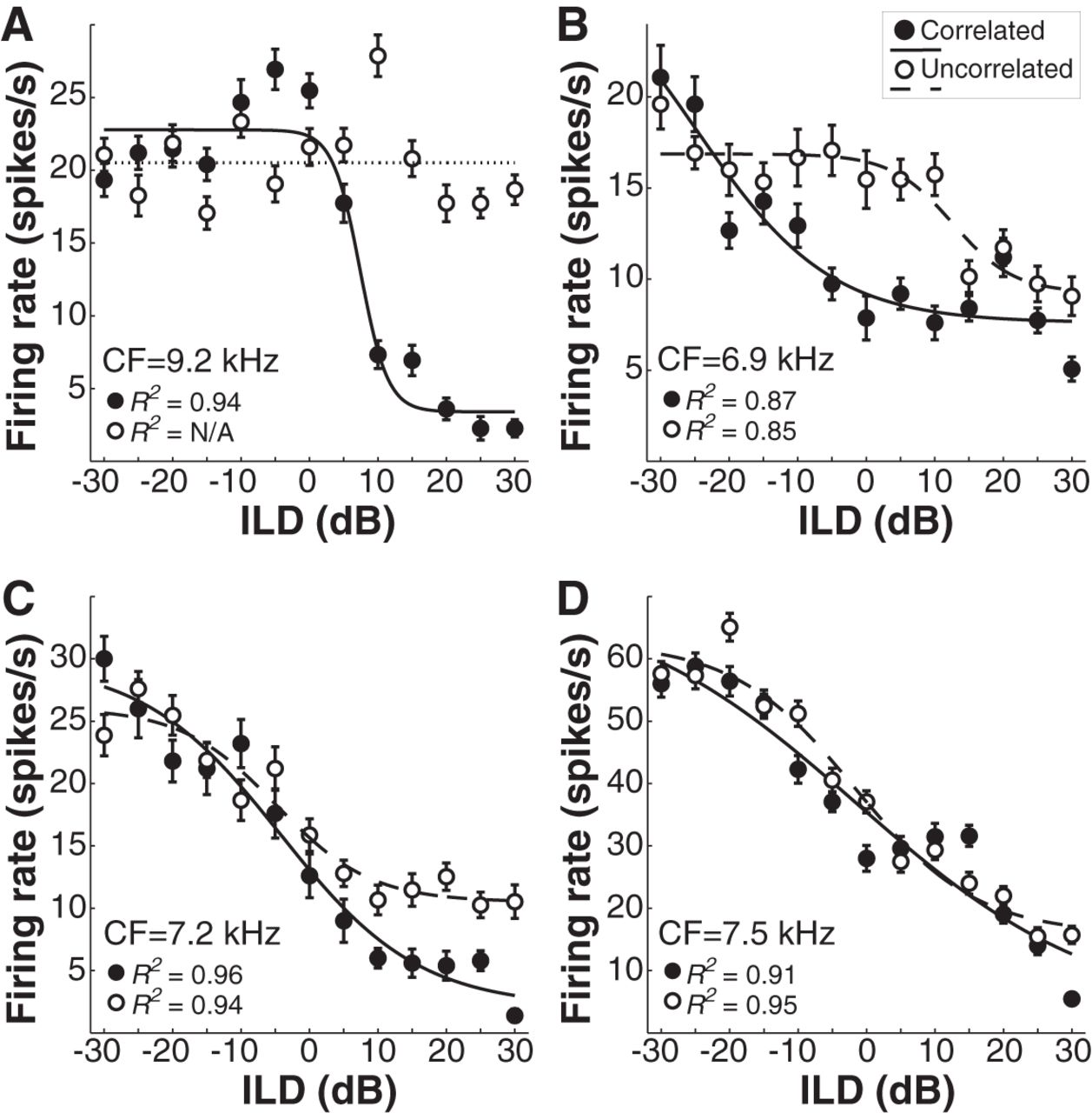
Recordings with broadband noise tokens were obtained from 34 ILD-sensitive ICC neurons (CFs 0.21–12.1 kHz, mean 5.7 kHz; thresholds 5–40 dB, mean 22.5 dB). In each neuron, rate-ILD functions were measured with both correlated and uncorrelated tokens. Figure 3 displays rate-ILD functions for 4 representative neurons of varied CF. ILD tuning was generally well described by a sigmoidal function, with firing rate decreasing systematically as the level of the ipsilateral stimulus increased. ILD tuning was remarkably unaffected by decorrelation, even in neurons with relatively low CFs that would be expected to receive inputs phase-locked to the stimulus fine-structure (Fig. 3C,D). A few (5 of 34) neurons lost their ILD tuning following decorrelation, including two units with very low CFs of 0.21 and 0.31 kHz (data not shown), but recordings from other very low CF neurons (where natural ILD cues are generally small, although see Jones et al., 2015) were not obtained. Across the 29 neurons that maintained significant tuning for both correlated and uncorrelated tokens, the best ILD JND per neuron (computed from FI using Eqs. 2, 3) increased on average by a factor of 1.36 (±0.14 SEM) for the uncorrelated stimulus.

ILD coding in ICC is robust to complete interaural decorrelation of broadband noise. A–D, Mean response rate (±1 SE) across ILD for correlated (filled circles) and uncorrelated (open circles) broadband noise tokens for four neurons of varied CF. Tuning was generally well-described by a four-parameter logistic function (solid line, correlated; dashed line, uncorrelated).
However, a likely source of variability in measured tuning functions and corresponding ILD JNDs in this set of experiments was the change in excitatory drive between correlated and uncorrelated conditions due to a change in the excitatory token used in the two cases (also true in previous measurements of ILD coding for uncorrelated stimuli: Egnor, 2001; Tollin and Yin, 2002; Devore and Delgutte, 2010). Such a change might also be elicited simply by presentation of different correlated tokens. To address this issue and to enable more targeted manipulation of the stimulus at unit CF, we next completed a series of experiments using narrowband noise tokens.
Neural ILD sensitivity persists for narrowband amplitude-modulated noise
Recordings with narrowband noise tokens were obtained from 32 ILD-sensitive ICC neurons (CFs 0.78–12.9 kHz, mean 6.0 kHz; thresholds 15–55 dB, mean 37.9 dB). In this set of experiments, two narrowband noise tokens were generated at each isolated unit's CF. The stimulus to the contralateral ear was fixed between “correlated” and “uncorrelated” conditions, thus restricting the change in stimulation to the ipsilateral (putatively inhibitory) ear. Like stimuli in psychophysical Experiment 1, stimuli were amplitude-modulated with 100 Hz narrowband noise (Fig. 1), thus potentiating large mismatches in the peaks of uncorrelated contralateral and ipsilateral stimulus envelopes. Figure 4A shows spike rasters for correlated (upper) and uncorrelated (lower) stimuli from a representative neuron tested with narrowband noise (CF = 3.6 kHz). Figure 4B shows a rate-ILD function for the same neuron. The uncorrelated ipsilateral stimulus elicited a slight increase in firing rate at most ILDs, but firing was still inhibited at ipsilateral-favoring ILDs, and the tuning statistics were very similar between the two conditions (correlated: half-maximal ILD = 5.3 dB; max-min dynamic range = 5.1 dB [69% modulation]; uncorrelated: half-maximal ILD = 7.3 dB; max-min dynamic range = 4.4 dB [63% modulation]). Correspondingly, ILD coding acuity, as assessed via the FI-derived neural ILD JND (see Materials and Methods), was nearly the same in the 2 cases (Fig. 4B, inset; correlated best JND = 2.6 dB ILD; uncorrelated best JND = 2.9 dB ILD). This pattern of minimal change with decorrelation was observed across the population of neurons in the sample, with only 1 neuron (1 of 32) losing its ILD tuning as a result of decorrelation. Across the 31 neurons that maintained significant tuning for both correlated and uncorrelated tokens, the best ILD JND per neuron increased on average by a factor of 1.80 (±0.39 SEM). This result was consistent with the small but significant psychophysical effect of decorrelation using comparable stimuli (Fig. 2), but surprising from an ILD coding perspective given the high degree of excitatory-inhibitory temporal mismatch produced by slow (100 Hz) uncorrelated envelope fluctuations. The effective overlap of excitation and inhibition for such stimuli apparently remained sufficient to enable ILD coding. We thus next devised stimuli that further degraded the timing of excitation and inhibition in an attempt to “break” the decorrelation-resistant ILD coding mechanism.

ILD tuning and neural discrimination performance in ICC are robust to interaural decorrelation of amplitude-modulated narrowband noise. A, Spike rasters for correlated (top) and uncorrelated (bottom) narrowband noise tokens. The contralateral (putative excitatory) noise token was fixed across conditions, whereas the ipsilateral (putative inhibitory) token was varied. B, Rate-ILD functions for correlated (filled symbols) and uncorrelated (open symbols) narrowband noise, drawn from the rasters in A. Inset, Neural ILD JNDs (heavier lines), derived using Fisher information (lighter lines) for correlated (solid) and uncorrelated (dashed) stimuli.
In some neurons, ILD sensitivity persists for temporally independent GCTs
Recordings with GCTs, which constrained signal energy to temporally discrete yet narrowband Gabor clicks (see Materials and Methods), were obtained from 17 ILD-sensitive ICC neurons (CFs 2.4–12.5 kHz, mean 6.5 kHz; thresholds 0–55 dB, mean 24.1 dB). As for narrowband amplitude-modulated noise stimuli, two stimulus tokens were generated at the CF of each isolated neuron, with the isochronous 10 ms ICI stimulus to the contralateral ear fixed, while a temporally jittered (10 ± 4 ms ICI) token was presented to the ipsilateral ear in the “independent” condition (Fig. 1). “Independent” stimuli included up to 4 ms of contra-ipsi temporal mismatch, potentiating epochs of excitation lacking opposing inhibition, and were therefore expected to significantly degrade ILD tuning. Figure 5 displays rate-ILD functions that represent the range of neural responses observed with GCT stimuli. ILD tuning was completely eliminated by temporal mismatch in some neurons (Fig. 5A), modestly degraded in other neurons (Fig. 5B,C), and remarkably unaffected in other neurons (Fig. 5D). Across the 8 neurons that maintained significant tuning for both correlated and uncorrelated tokens, the best ILD JND per neuron increased on average by a factor of 5.37 (±2.33 SEM), or by a factor of 3.31 (±1.23 SEM) excluding one neuron that gave a 20-fold increase in minimum JND with independent GCTs. Collectively, GCT measurements suggest significant variability in the effective excitatory-inhibitory integration times of ILD-sensitive ICC neurons, with evidence for highly integrative neurons capable of encoding ILD in temporally independent signals (see Discussion). We explicitly examine the matter of excitatory-inhibitory temporal windows in the following sections. Population summary data for neurons tested with 10 ms ICI GCTs are given in Figure 6I–L, along with summary data for broadband noise (Fig. 6A–D) and narrowband noise (Fig. 6E–H).

Summary ICC responses across stimulus types demonstrate remarkable robustness to decorrelation. A, Mean logistic rate-ILD functions for neurons tested with correlated (solid line, shading ±1 SE) and uncorrelated (dashed lines) broadband noise. Rates were normalized for each neuron to the maximum of the function for correlated stimuli. Five units lost ILD tuning with decorrelation (numbers in top right; see Results). B, Rate modulation across neurons for correlated (filled circles) and uncorrelated (open circles) broadband noise. A value of 1.0, rarely observed, means that firing was completely inhibited at sufficiently ipsilateral-favoring ILDs. C, Average Fisher information per cell, derived from 1000-repeat bootstrap estimates of total population Fisher information. Error bars indicate bootstrapped 95% CIs for correlated and uncorrelated broadband noise (shading indicates correlated error bars: thin dashed lines indicate uncorrelated error bars). Inset, To calculate population FI, each cell and corresponding rate-ILD function (from Eq. 1; left panel, thin black trace) is assumed to have a mirrored equal (thin gray trace) in the opposite ICC; FI (from Eq. 2) is then taken as the sum of the FI of “left” and “right” cells (middle), from which the neural JND (from Eq. 3) can also be derived (right panel). Across the population, FI per cell is thus the mean of summed “left” and “right” populations divided by the number of cells per population. D, Mean ILD JND per cell, computed from C using Equation 3. E–H, Identical to A–D, but for amplitude-modulated narrowband noise tokens. I–L, Identical to A–D, but for 10 ms ICI GCTs.
Bilateral excitatory-inhibitory integration windows in ILD-sensitive ICC neurons
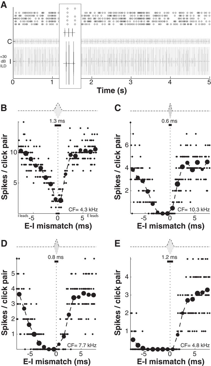
In this set of experiments, neurons were first presented with tones at unit CF to measure conventional rate-ILD functions. Once ILD sensitivity was established, two 5 s GCTs were generated at the unit CF. The contralateral stimulus was isochronous, with a fixed 20 ms ICI; the ipsilateral stimulus was temporally jittered with an ICI of 20 ± 8 ms, with ipsi-contra mismatch defined for each click pair in the sequence (see Fig. 1, bottom). Stimuli were then presented at an ipsilateral-favoring ILD of +30 dB, expected to reliably inhibit spiking given 0 ms contra-ipsi mismatch. Stimuli were repeated five times (five trials) per neuron. A total of 18 neurons were characterized using this method (CFs 1.2–11.6 kHz, mean 6.4 kHz; thresholds 10–50 dB, mean 30.8 dB). Figure 7A illustrates an example spike-time raster, with an enlarged view of a brief segment in which large (click pair numbers 1, 3) or small (click pair 2) ipsi-contra temporal mismatch resulted in either spiking or inhibition of spiking.

ICC neurons exhibit several-millisecond duration windows of excitatory-inhibitory interaction. A, An example raster for the 5 s duration 20 ms ICI GCT stimuli used to assess windows of E-I interaction. Despite a +30 dB ipsilateral-favoring ILD, the contralateral stimulus reliably elicits spikes when the ipsilateral (putative inhibitory) stimulus is sufficiently mistimed. B–E, Each panel plots the number of spikes elicited by each of 240 click pairs (smaller points) with given contra (E)–ipsi (I) temporal mismatch. Mean spike count per 1 ms bin of temporal mismatch is given by the larger points, with the size of each mean point scaled by the number contributing observations. Because Gabor clicks had non-negligible duration (dependent on CF), the effective duration of E-I stimulus overlap is indicated by the black bar above each panel. Window width was computed by subtracting this value from the FWHM of a Gaussian fit to mean spike count data (see Materials and Methods, Results).
Figure 7B–E illustrates responses from four neurons spanning the range of temporal window widths observed in our sample, from narrow (Fig. 7B) to broad (Fig. 7E). Small points plot values for individual click pairs; larger points plot averages across 1 ms bins (the size of each point is weighted by the number of click pairs in that bin). A single Gabor click (and its envelope, dashed line) is illustrated above each window. The number and black bar below each click show the half-width, in milliseconds, of the autocorrelation of the signal envelope, which decreased with increasing CF due to the fixed approximately one-third octave stimulus bandwidth. This purpose of computing this value was to account for the significant stimulus overlap that occurred at putative nonzero values of ipsi-contra mismatch, especially at lower CFs for which click durations were longer. In effect, the computed value defines a “zero-mismatch region” in which the stimuli can be considered to be overlapping even though their peaks are misaligned. E-I window width was then quantified using Equation 4 (as described in Materials and Methods), taken as the FWHM of a fit Gaussian less the duration of stimulus overlap (black bar).
Excitatory-inhibitory temporal windows are uniformly longer in ICC than reported in LSO
Figure 8A plots the population mean normalized window (±1 SD) for our sample of ICC neurons (black lines). Overlaid on this window is the mean (±1 SD, gray shading) of 10 previously reported LSO windows measured in vivo using broadband transients (Joris and Yin, 1995; Park, 1998; Irvine et al., 2001; very similar in vitro measurements were reported by Wu and Kelly, 1992). The LSO temporal windows, though drawn from 3 different studies and model species, appear remarkably homogeneous and substantially narrower than windows observed in ICC. To enable a more quantitative comparison, LSO window data were fit in the same manner described above for ICC windows. Figure 8B displays computed window widths for both ICC (black) and LSO (gray), ordered from narrowest to widest. The distributions are non-overlapping, with the narrowest windows in our ICC sample at ≥2 ms, compared with LSO windows which are uniformly <l ms (cf. Park, 1998) (see Discussion). This spread of window widths in ILD-sensitive neurons along the neuraxis is of interest with respect to behavioral performance and led us to examine the effect of window width on ILD sensitivity parametrically.

Temporal windows of integration are longer in ICC than in LSO. A, Mean temporal window (±1 SD) for ICC neurons of the present study (black lines) and for 10 LSO neurons from 3 previous studies (asterisk; Joris and Yin, 1995; Park, 1998; Irvine et al., 2001). B, Distributions of window widths in ICC neurons of the present study and previously reported LSO neurons, each computed using Equation 4.
Narrow temporal windows precipitate degraded ILD sensitivity for decorrelated stimuli
We studied the effect of binaural temporal window width on ILD sensitivity using (1) a rudimentary model of ILD processing (see Materials and Methods) and (2) a second psychophysical experiment. In both cases, stimuli were GCTs similar to those used in physiological experiments, with the exception that stimuli were temporally jittered bilaterally, either identically or independently. Jitter was imposed in both channels (rather than only one, as in physiological experiments) to avoid the introduction of timbral differences between the ears in the psychophysical experiment.
Figure 9A illustrates our usage of the Zilany auditory nerve model (Zilany et al., 2009, 2014), with example model outputs for 4 ms ICI GCT stimuli. The model was run for parallel “excitatory” and “inhibitory” channels. In the example illustrated, the ILD favors the inhibitory channel by 10 dB. Firing should thus be inhibited, given by few spikes (bold lower traces) falling out of the window of E-I integration. Effective ILD coding is illustrated in Figure 9A (left) for binaurally identical inputs, with a temporal integration window of 1 ms. When this same 1 ms window is applied to binaurally independent GCT inputs, however, the excitatory stimulus “leaks through” the E-I process, and significant spiking occurs (Fig. 9A, middle). An increase in the duration of the integration window (to 8 ms, in this example) reduces the leakage of excitation, and enables effective computation of the ILD despite the temporal independence of E and I inputs (Fig. 9A, right).

Rudimentary model elucidates significance of “slow” temporal integration in ILD processing. A, Inputs to the model, consisting of spike trains generated by the Zilany et al. (2009, 2014) auditory nerve model (see Materials and Methods). In this example, spike trains are shown for 4 ms average ICI GCT stimuli that were binaurally identical (left panel) or independent (two right panels). One channel is assigned a positive (excitatory) value, the other a negative (inhibitory) value. The output is then the sum of E and I within a running temporal window of varied duration (“sliding” bar in each panel), with the result half-wave rectified to eliminate negative spikes (Eq. 5). For example, when stimuli are identical, an inhibition-favoring ILD of 10 dB yields few spikes, even with a short (1 ms) integration window (left). When stimuli are temporally mismatched, however, a large number of spikes leak through the E-I process (middle). A longer (slower) window enables recovery of the inhibition-favoring ILD (right). B, Model outputs for identical and independent GCTs with ICIs of 2, 4, and 8 ms, with window width varied from 1 to 32 ms. Input ILD was varied to enable the generation of simulated rate-ILD curves (normalized to the response rate for the excitatory stimulus alone).
Figure 9B illustrates model computations for GCT inputs with 3 different ICIs as a function of ILD. The top row gives normalized (to E alone) rate-ILD functions for “identical” inputs, with temporal integration window width as the parameter; the bottom row gives rate-ILD functions for “independent” inputs. There is little or no effect of window width given identical inputs. Given independent inputs, the effect of window width is readily apparent. Short temporal windows enable dramatically more excitation to pass through the E-I process when E and I inputs are mistimed, leading to poor encoding of the ILD cue for “decorrelated” stimuli, with poorer coding for higher degrees of decorrelation (achieved, in this case, via increases in the average ICI).
To quantify the effect of temporal window width on ILD coding acuity, computed rate-ILD functions (Fig. 9B) were transformed into FI-based JND functions using Equations 2 and 3. Absolute JND values were not of interest; rather, we were interested in assessing the relative effect of E-I temporal mismatch across window widths for each ICI. Figure 10 illustrates our derivation of these values, with predicted increases in JND for each window width given in Figure 10B. The deleterious effect of narrow window widths on ILD detection performance (for a shift in the ILD cue away from midline) is clear, with expectedly more dramatic effects at longer ICIs where greater E-I mismatches are possible.
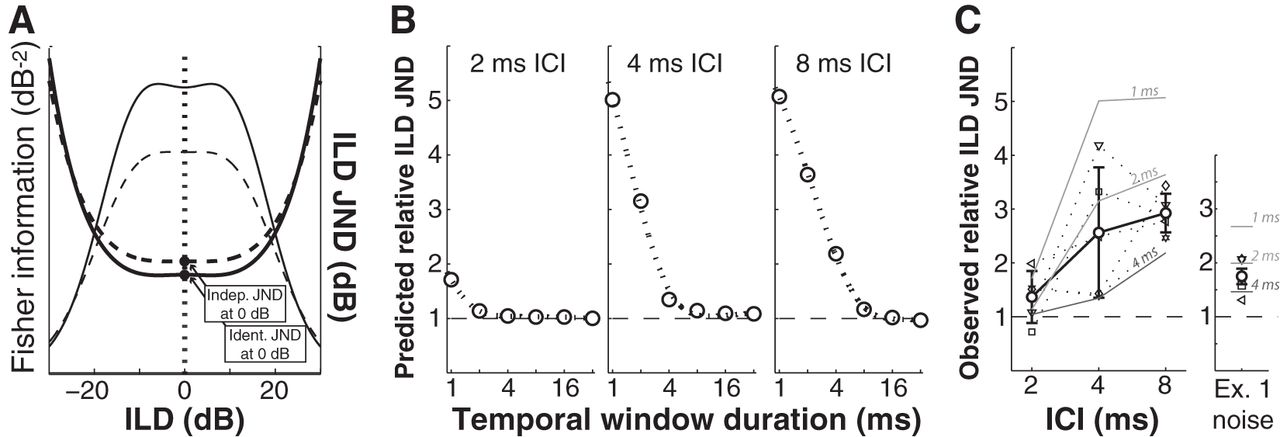
Comparison of model predictions and psychophysical data suggests an ILD integration window of ∼3 ms. A, Model responses were used to generate Fisher information-based (thin lines) ILD JNDs (thicker lines) for identical (solid lines) and independent (dashed lines) stimuli. B, A predicted relative ILD JND for each stimulus passed through the model (GCTs of 2, 4, and 8 ms) was generated by normalizing independent to identical model ILD JNDs for each window size. C, A second psychophysical experiment was conducted to measure these values empirically in 5 human subjects. For comparison, model predictions using three different temporal window durations (1, 2, and 4 ms) are indicated (labeled grayscale lines). ILD JNDs increased across ICI, with the observed mean effect falling between model predictions for 2 ms and 4 ms integration windows (left). The same pattern was evident for data from the first psychophysical experiment using narrowband noise stimuli (right).
Psychophysical effect of increasing temporal mismatch elicited using jittered GCTs
Data for a second psychophysical experiment (Experiment 2; see Materials and Methods) that used the same jittered GCT stimuli passed through the model are given in the left panel of Figure 10C. Five human subjects, four of whom had participated in Experiment 1, were tested in a simple adaptive ILD discrimination task using identical and independent GCT stimuli with ICIs of 2, 4, and 8 ms. As for the model (Fig. 10B), data are given as thresholds for independent stimuli normalized to thresholds for identical stimuli. As for model responses, the relative effect of interaural decorrelation increased with increasing ICI. At a nominal ICI of 8 ms, performance was approximately threefold worse for independent than for identical stimuli, a decrement more severe than predicted given a 4 ms temporal window, but less severe than predicted given a 2 ms temporal window. Indeed, the mean effects of E-I mismatch for the GCT stimuli of Experiment 2 (Fig. 10C, left) and also for the 100 Hz amplitude-modulated narrowband noise stimuli of Experiment 2 (thresholds replotted as normalized values in Fig. 10C, right) are consistent with an E-I integration window of ∼3 ms. This window duration is approximately threefold longer than observed in neurons of the LSO (Fig. 8) but consistent with the lower end of window durations observed in neurons of ICC. The implications of this and the foregoing findings are discussed in the remaining sections.
Discussion
Neurons of the ICC are extremely robust to interaural decorrelation
A principal finding of the present study is that ILD-sensitive neurons of the ICC are nearly immune to even complete interaural decorrelation, a stimulus manipulation that renders ITDs undetectable for both neurons (Yin et al., 1986; cf. Devore et al., 2009) and psychophysical subjects (Rakerd and Hartmann, 2010). Previous neurophysiological studies showed little effect of decorrelation on ILD sensitivity but used either broadband unmodulated noise (Egnor, 2001; Tollin and Yin, 2002) or only partially decorrelated noise (Devore and Delgutte, 2010) and reported data for only high-CF neurons (CFs > 3 kHz). We found that total decorrelation of both broadband noise and narrowband amplitude-modulated noise affected ILD sensitivity very little across nearly all neurons in our sample, including some low-CF neurons (Fig. 3C,D), with mean neural ILD JNDs increasing only slightly as a result of interaural decorrelation (Fig. 6D,H). Indeed, a subset of neurons (n = 8 of 17) remained capable of encoding ILDs carried by temporally independent click trains (Fig. 6I–L), although degradations of sensitivity were larger than for noise tokens, with the mean neural JND increasing more than threefold (see Results; Fig. 6L). Such integrative coding differs from that observed at the primary site of ILD sensitivity in the brainstem, the LSO (cf. Park, 1998; see below). Indeed, it is interesting to consider why such a temporally precise E-I circuit is maintained at the level of LSO if this precision may limit ILD coding. Two ideas are that, apart from ILD coding, fast E-I processing in LSO contributes to the encoding of ITD (Joris, 1996; Tollin and Yin, 2005), or the encoding of amplitude modulation for both monaural and binaural signals (see Ashida et al., 2016).
Behavioral ILD sensitivity is consistent with several-millisecond windows of E-I interaction
Previous psychophysical measurements in human (Hartmann and Constan, 2002) and animal subjects (Egnor, 2001; Keating et al., 2013) indicated that psychophysical detection of ILDs was essentially unaffected by decorrelation. These experiments used broadband stimuli that conveyed information in many auditory filters simultaneously and did not assess the usability of suprathreshold information (e.g., for lateralization). The present psychophysical data demonstrate that, even when signal energy is confined to a single auditory filter and inhibitory and excitatory stimulus envelopes fluctuate independently, the detectability and salience of the ILD cue are very minimally affected (Fig. 2). These data are in some ways reminiscent of previous psychophysical measurements suggesting that ILDs carried by rapidly fluctuating amplitude-modulated signals can be temporally averaged to facilitate detection (cf. Brown and Stecker, 2010; Stecker and Brown, 2012). Cross-comparison of our psychophysical, physiological, and modeling data points to an effective window of ILD integration of at least ∼3 ms. This estimate may not capture secondary stages of integration (e.g., cross-frequency integration), which might contribute to longer estimated integration times and smaller measured JNDs in previous studies using broadband stimuli (cf. Hartmann and Constan, 2002). Nonetheless, the temporal robustness of ILD sensitivity reported here should be sufficient to enable detection of ILD carried by any ecological signal, including signals in highly reverberant environments, where values of interaural correlation approach 0.1–0.2 (Hartmann et al., 2005). As reverberation also reduces the magnitude of ILD cues (Shinn-Cunningham et al., 2005; Devore and Delgutte, 2010), maintenance of sensitivity to small changes in ILD under reverberant conditions may be particularly important. From a human clinical perspective, integrative coding could also contribute to the preservation of ILD sensitivity for bilateral device-processed signals, which are typically unsynchronized between the ears, potentiating temporal distortions (Brown et al., 2016) that may impact ITD but not ILD sensitivity (Grantham et al., 2008).
Previous studies of E-I interaction in ICC
Previous studies have evaluated windows of binaural E-I interaction in neurons of the ICC (Benevento and Coleman, 1970; Carney and Yin, 1989; Irvine et al., 1995; Kidd and Kelly, 1996; Park, 1998; van Adel et al., 1999). Such measurements have generally been made (1) with single transients, in the context of ITD processing (see below) and (2) under barbiturate anesthesia, which dramatically alters the extent and time course of inhibition in the ICC (Kuwada et al., 1989; Tollin et al., 2004; Song et al., 2011; Chung et al., 2014). Consistent with the effects of barbiturate anesthesia, very long windows of interaction (≥30 ms) have been reported in a number of studies (Carney and Yin, 1989; Kidd and Kelly, 1996 van Adel et al., 1999). However, in a study of LSO versus IC ILD sensitivity in bat wherein animals were allowed to recover from barbiturate anesthesia before recording, Park (1998) found that the so-called “duration of excess inhibition,” the temporal window of complete inhibition in EI neurons, was 3.1 ms in ICC and only 0.4 ms in LSO. In our sample, collected under ketamine/xylazine anesthesia, which exerts minimal effects of ICC responses (Astl et al., 1996), only a few E-I windows exhibited any “excess inhibition” (completely inhibited firing at non-zero mismatches; Fig. 7E), even at a 30 dB ipsi-favoring ILD. Windows of the present study thus appear somewhat narrower than measured in previous ICC studies. Nonetheless, all ICC studies to date suggest E-I window widths on the order of multiple milliseconds rather than hundreds of microseconds (cf. Tollin et al., 2004), and thus uniformly longer E-I windows in ICC than LSO.
Origins of long binaural E-I windows in ICC
Although our data do not provide a mechanistic explanation for the long E-I windows we measured in ICC, a very likely candidate mechanism is GABAergic inhibition via inputs from DNLL (Kidd and Kelly, 1996), also called “persistent inhibition,” extensively studied by Pollak and colleagues (see Pollak, 2012). Iontophoretic application of bicuculline, a GABA receptor antagonist, blocks the effect of persistent inhibition in ICC (Burger and Pollak, 2001; Pecka et al., 2007). Kidd and Kelly (1996) explicitly demonstrated that pharmacological blockade of contralateral DNLL via injection of kynurenic acid in DNLL led to shorter windows of E-I interaction (that later recovered to preinjection width), indicating an essential role for DNLL-based inhibition in shaping E-I interactions in ICC. The shape of our windows, clearly skewed toward negative (inhibition-favoring) E-I mismatches (Figs. 7B–E, 8), is consistent with such persistent inhibition. Other mechanistic explanations are possible, such as convergent input to a single IC neuron from two or more LSO neurons with differently tuned E-I windows. Given the heterogeneity of ILD-coding circuits in ICC (Pollak, 2012; Li and Pollak, 2013), it is indeed likely that multiple mechanisms contributed to the windows we and others have measured.
“Fast ILD” sensitivity versus ITD sensitivity
E-I neurons that are systematically modulated by ITD generally exhibit discharge peaks when the inputs are maximally out of phase (i.e., at a “characteristic phase” of 0.5 cycles; Tollin and Yin, 2002) and prominent discharge minima when inputs are in phase. Indeed, previous reports of E-I windows for transients have typically plotted the relative timing of ipsilateral and contralateral inputs explicitly in terms of ITD (Carney and Yin, 1989; Kidd and Kelly, 1996; Irvine et al., 2001). The functional role of E-I neurons in ITD coding has been discussed previously (Grothe et al., 2010), but Joris (1996) raised the interesting notion that E-I-type ITD sensitivity in LSO neurons may be “nothing else than ‘fast’ ILD sensitivity.”
While the temporal windows generated in the present study likely could have been generated using single transients varied in “ITD” or by presenting binaural beat-like click train stimuli, this study was not developed in the context of ITD coding. Rather, the temporally jittered click trains we used intentionally lacked orderly changes in ITD, in the interest of producing an extreme example of interaural decorrelation. Although it would be accurate to plot the measured windows in terms of ITD, the windows are defined on a scale of milliseconds rather than microseconds, or, from an ecological standpoint, on the scale of millisecond fluctuations due to reverberation, echoes, superposed signals, and other sources of temporal asynchrony, rather than microsecond shifts in signal timing between the ears due to sound source azimuth. To recast the point raised by Joris (1996), the ILD sensitivity of many E-I neurons in the ICC is apparently not very “fast,” and their resultant E-I temporal tuning functions may be more sensibly viewed as windows of binaural integration rather than ITD sensitivity curves.
Limitations of the present study
Our study compared behavioral data from human listeners with neurophysiological data from a rodent model, the chinchilla. While chinchillas were selected for the audiometric similarity to humans, including a similar range of hearing (Heffner and Heffner, 1991) and demonstrated use of both ITD and ILD cues for sound localization (Heffner et al., 1994), such cross-species comparisons are, of course, limiting. The effect of interaural decorrelation on ILD sensitivity appears to be similarly negligible in humans (present study; Hartmann and Constan, 2002) and ferrets (Keating et al., 2013), and also barn owls (Egnor, 2001), but behavioral data from chinchilla or other animal models could be informative, if only to further confirm the lack of an effect. Although aspects of our behavioral and midbrain neural data were similar, other explanations for integrative ILD sensitivity (e.g., involving downstream mechanisms we did not consider) could certainly be proposed (Stecker et al., 2015). Finally, although effects of ketamine anesthesia on ICC neuronal responses appear to be minimal (Astl et al., 1996), it would be desirable to obtain data from an unanesthetized/awake preparation for comparison with the present and previous data.
Footnotes
This work was supported by National Institute for Deafness and Communication Disorders, National Institutes of Health Grant F32-DC013927 to A.D.B. and Grant R01-DC011555 to D.J.T. We thank Drs. Nate Greene, Victor Benichoux, and Chris Stecker for many helpful discussions on mechanisms and models of ILD coding; and Brianne Beemer, Kelsey Anbuhl, and Alex Ferber for technical assistance.
The authors declare no competing financial interests.
- Correspondence should be addressed to Dr. Andrew D. Brown, University of Colorado School of Medicine, Department of Physiology and Biophysics Research Complex 1-N, Room 7401G, 12800 East 19th Avenue, Aurora, CO 80045. Andrew.D.Brown{at}ucdenver.edu


