

Abstract
Noise, which is ubiquitous in the nervous system, causes trial-to-trial variability in the neural responses to stimuli. This neural variability is in turn a likely source of behavioral variability. Using Hidden Markov modeling, a method of analysis that can make use of such trial-to-trial response variability, we have uncovered sequences of discrete states of neural activity in gustatory cortex during taste processing. Here, we advance our understanding of these patterns in two ways. First, we reproduce the experimental findings in a formal model, describing a network that evinces sharp transitions between discrete states that are deterministically stable given sufficient noise in the network; as in the empirical data, the transitions occur at variable times across trials, but the stimulus-specific sequence is itself reliable. Second, we demonstrate that such noise-induced transitions between discrete states can be computationally advantageous in a reduced, decision-making network. The reduced network produces binary outputs, which represent classification of ingested substances as palatable or nonpalatable, and the corresponding behavioral responses of “spit” or “swallow”. We evaluate the performance of the network by measuring how reliably its outputs follow small biases in the strengths of its inputs. We compare two modes of operation: deterministic integration (“ramping”) versus stochastic decision-making (“jumping”), the latter of which relies on state-to-state transitions. We find that the stochastic mode of operation can be optimal under typical levels of internal noise and that, within this mode, addition of random noise to each input can improve optimal performance when decisions must be made in limited time.
Introduction
Trial-to-trial variability, considered ubiquitous in neuronal systems (Shadlen and Newsome, 1998), can obscure the nature of the dynamics of a single-trial neural response to a sensory stimulus (Durstewitz and Deco, 2008). In particular, if neural processing involves sharp transitions between discrete states and if the timing of the transitions varies from trial to trial, then these transitions become broadened by analyses such as principal component analysis (PCA) that first combine data across trials to form peristimulus time histograms (PSTHs). Analyses such as Hidden Markov modeling (HMM) (Abeles et al., 1995; Seidemann et al., 1996; Jones et al., 2007), meanwhile, are not anchored to the time point of stimulus delivery and so have no difficulty incorporating such trial-to-trial variability. If state transitions are real properties of the data, HMM can use correlations in firing-rate changes of multiple cells across transitions regardless of whether the transitions occur at identical poststimulus times in each trial; thus, HMM extracts more information about such neuronal responses than PSTH-based methods.
Recently, we documented the existence of just these kinds of ensemble responses in gustatory cortex (GC) during taste processing (Jones et al., 2007). HMM of ensemble neural data from GC provided more information on taste identity than standard ensemble PCA and other PSTH-based analyses. Such a result suggests that each taste does in fact produce a reliable sequence of relatively long-lived (200–1000 ms) states with fast transitions (averaging 60 ms) between them. Transition times vary from trial to trial (by up to the mean lifetime of states) such that averaging of firing rates across trials reveals only an artifactually smoothly varying response.
Here we place these empirical findings in a solid computational framework, demonstrating that such neural activity can arise from the timing of stochastically induced, rapid changes between discrete, deterministically stable network states (Okamoto et al., 2007; Miller and Wang, 2006; Deco et al., 2007b, 2009; Gigante et al., 2009). Our attractor-based model network possesses the key features of neural activity observed during taste processing (Jones et al., 2007). (1) Transitions between states produce correlated, rapid changes in firing rates of multiple neurons. (2) Transitions occur at discrete but unpredictable times in individual trials. (3) Much slower variations of activity are observed in PSTHs. (4) Individual stimuli bias the transitions through reliable sequences of states.
To study the computational advantage of network dynamics based on stochastic transitions between discrete states, we also investigate a reduced network that performs winner-takes-all decision-making (Wang, 2001), representing a categorical perception of one taste over another (or the two-alternative forced choice of “spit” vs “swallow”) evident in neural activity of GC as a palatability response (Katz et al., 2001; Fontanini and Katz, 2006; Grossman et al., 2008). We modulate the excitability of the network to change its operating mode from one of deterministic integration (“ramping”) to one in which the spontaneous state remains stable and decisions are made by stochastic transition (“jumping”). We measure how reliably the probabilistic binary responses follow small input biases favoring one outcome over another and demonstrate that the jumping mode is optimal under many conditions.
Materials and Methods
Model network simulations: taste-processing network.
Our model taste-processing network (Fig. 1) is designed to mimic the cortical neural responses observed during the processing of two tastes of opposite palatability (such as sucrose and quinine): specifically, cell groups whose activity increases in one of the three epochs of taste processing (Katz et al., 2001; Fontanini and Katz, 2006), which we label “detection,” “identification,” and “decision.” For the simplified model, one group of cells is necessary for detection and two each for the identification and decision, so our base network has five groups. Each group of cells comprises an excitatory population and an inhibitory population in a 4 to 1 ratio in correspondence with cortical data. Unless otherwise stated, a total of 100 cells per pool is used (80 excitatory and 20 inhibitory). Specific connection strengths are given in the supplemental data (available at www.jneurosci.org as supplemental material).

Architecture of model network for taste processing. A, The model network is based on five pools of neurons, with each pool containing NE excitatory cells and NI = NE/4 inhibitory cells (by default, NE = 80, NI = 20). Recurrent excitatory connections (data not shown) dominate within a pool. Arrows indicate significant excitatory connections between pools, and balls indicate the strong cross-inhibition between pools that produce one binary decision of palatability. Other connections (data not shown) produce weak inhibition between all pools. Recurrent excitation is sufficient to maintain the activity of a pool, once a combination of inputs and random fluctuations has driven the pool into an active state. The network progresses through the three epochs of detection (somatosensory response), identification (chemosensory response), and decision (palatability response) that are observed in gustatory cortex during taste processing. Each successive epoch is driven by strong activity arising in a particular pool, which through cross-connections alters the activity in all pools. B, C, Trial-averaged firing rates of four cells in the model network, after a stimulus representing either taste 1 (B) or taste 2 (C). Color of the trace indicates the pool from which the cell is taken. Note the gradual ramping of firing rates that can take >1 s for some cells.
We simulate taste delivery by adding Poisson spike trains to all excitatory cells in the taste-processing network, beginning at a time of 100 ms after stimulus (representing the delay from taste delivery to neural responses in gustatory cortex). The two tastes were distinguished by the cells in one of the two pools labeled “taste” in our model network (Fig. 1A) receiving inputs at a 20% higher rate than the otherwise symmetric pool. For additional details, see the supplemental data (available at www.jneurosci.org as supplemental material).
Model network simulations: decision-making network.
The decision-making network is a subsection of the taste-processing network that is designed to produce a palatability response upon receiving input from cells with information pertaining to taste identity. That is, we designed the subnetwork to analyze just one of the multiple transitions in the full taste-processing network: the transition from “identity” to “palatability”. A similar decision-making network could underlie the transition from “detection” to “identity” in taste processing.
Our network has the structure of previous model networks for decision-making (Wang, 2002; Wong and Wang, 2006; Wong et al., 2007): competing pools of excitatory neurons with strong self-excitation and strong cross-inhibition. As with the full taste-processing network, each excitatory pool of cells is coupled with one-fourth the number of inhibitory cells (rather than a global inhibitory network as in some models). The self-excitation generates an attractor state of high activity for each pool, such that with sufficient input they are excited from a stable state of low firing-rate, spontaneous activity to the highly active state. The cross-inhibition ensures that only one of the excitatory pools can be active at a time (in the absence of overwhelming input). Details of the specific connections are given in the supplemental data (available at www.jneurosci.org as supplemental material).
We adjust the operational mode of the decision-making network, from ramping to jumping, by reducing its overall excitability, to render the spontaneous, low activity of each pool more stable. We achieve such a reduction in excitability by either reducing overall excitatory input during the stimulus or increasing the leak conductance of all excitatory cells (equivalent to a uniform inhibitory input). For Figures 5 and 6, we simultaneously altered several synaptic parameters (see Fig. 5 legend) to generate a network in the ramping mode that had sufficiently slow integration of inputs to match the timescale of the jumping network.
Model network simulations: single-cell properties.
Because HMM was applied to neural spike train data by Jones et al. (2007), our level of modeling is sufficiently realistic that neural spike trains are produced. Beyond this, model specification is minimal, however: we do not assume that any particular property of a single neuron is responsible for the observed temporal dynamics. The multiple timescales of the system arise from the interaction between network structure and rapid noise fluctuations rather than from any specific property explicitly built into the model. Thus, we chose the simplest possible model of a spiking neuron, namely the leaky integrate-and-fire (LIF) model (Tuckwell, 1988). LIF cells fire at a higher rate with increased excitatory input once a threshold is reached and at a lower rate when inhibitory input is increased; they produce spike trains with a coefficient of variation similar to that of a Poisson process, assuming sufficiently noisy inputs. To ensure noisy spike trains, beyond the input explicitly calculated from cells within the network, we add a Poisson barrage of excitatory and inhibitory synaptic inputs to represent activity of other connected cells not explicitly included in our network.
The basic equation for the LIF neuron describes the temporal variation of membrane potential, Vi, of cell i, when receiving total excitatory synaptic conductance input gESiE, and total inhibitory conductance input gISiI, according to the following:
 where Ci is the membrane capacitance of the cell, gL is its leak conductance, VL is the leak membrane potential (respectively, the conductance across the cell membrane and the resting potential of the cell in the absence of synaptic input and spiking activity), VE is the reversal potential of excitatory synaptic input, and VI is that of inhibitory synaptic input. The scales of excitatory and inhibitory synaptic conductance are set by gE and gI, respectively, with maximal conductance of a synapse from neuron j to i given by gEWIi (if excitatory) or gIWIi (if inhibitory). Total synaptic inputs SiE and SiI are given by summing over presynaptic cells (over all excitatory cells to calculate SiE and over all inhibitory cells to calculate SiI):
 where sj is the fraction of receptors opened by the spikes of neuron j. We determine sj from
 where τs is the synaptic time constant, tjn is the time of the nth spike of neuron j and tj−n is the time just preceding that spike time. When the membrane potential reaches a threshold, VTh, a spike is recorded and the membrane potential is lowered to a reset value, VR, for a refractory period, τref. Equations were integrated using second-order Runge–Kutta with a time step of 0.1 ms.
Parameters were chosen such that, in the absence of explicitly modeled synaptic inputs, excitatory cells fired at under 3 Hz, whereas inhibitory cells fired at ∼5 Hz. Their specific values are given in the supplemental data (available at www.jneurosci.org as supplemental material).
Hidden Markov modeling.
We used standard Matlab packages for Hidden Markov modeling, using as inputs 10 trials of spike trains of two excitatory cells per pool (10 total) in the taste-processing network and four excitatory cells per pool (8 total) in the decision-making network (these numbers of trials and neurons are similar to those successfully analyzed by Jones et al., 2007). We binned spike trains on a scale of 2 ms and generated vectors containing the identity of a neuron that spiked in each bin, with a “0” for no spike. (For the rare occurrence of a bin containing spikes from more than one cell, neuron identity was chosen randomly from the cells that spiked.) We iterated until convergence or up to a maximum of 500 iterations, using the Baum–Welch algorithm, which is guaranteed to approach a local optimum, using eight different random starting models. The final model with maximum log likelihood (calculated as the probability of producing the measured spike trains given the particular model) was treated as the optimal characterization of population activity in the network. Given the final model, we were able to plot for each trial the probability as a function of time that the ensemble of neuronal activity corresponds to a particular HMM state.
For our baseline simulations we allowed six HMM states to be used in the modeling. In typical simulations of the taste-processing network, only four states were used in a trial, and, in the decision-making network, only two states were used. That is, HMM defined the probability of being in these extra states as 0 throughout trials. To test the importance of model parameters, we also ran HMM starting with from 3 to 10 states and with time bins varying from 1 to 25 ms. We calculated the overlap of these model outputs with our original model in cases when equivalent states could be observed. We defined the overlap, O(λ) in each trial (λ) as a normalized dot product between the probabilities P and P′ for the original and new HMM by the following calculation:
 where i is the index of the time bin (from 1 to N) in the original model, and the sum over n is the sum over states matched across models by their order of appearance. Thus, P′in(λ) is the probability in a comparison model, being in state n in trial λ at the time equal to the time of the ith bin in the original model (the actual bin number may be different when comparing models of different bin size). From the set of O(λ) across trials, we report the mean and SD in Results. Figures of example trials with specific parameters and values for O(λ) are provided in the supplemental data (available at www.jneurosci.org as supplemental material).
Performance of decision-making network.
For each parameter set, we simulated 100 random trials and defined performance as the number of correct minus the number of incorrect responses. We defined a response as the average firing rate of one pool exceeding that of the other pool by >20 Hz and the response as “correct” when the pool with greater input had the high firing rate.
Results
Stochastic transitions between discrete states
Our model network for taste processing produced a predictable sequence of activity states given a specific set of inputs, with sharp transitions between the states (Fig. 2A,B,D,E). Sequences were stable, with all 10 trials of each particular set of inputs producing an identical sequence (see also transition matrices in the supplemental data, available at www.jneurosci.org as supplemental material). We simulated two types of input corresponding to two different tastes, which produced two different sequences (although with an identical initial state). Average state duration was 615 ± 68 ms for taste 1 and 471 ± 50 ms for taste 2, whereas average transition time between states was smaller by more than an order of magnitude (mean of 27 ± 6 ms for taste 1 and mean of 35 ± 4 ms for taste 2).

Neural activity produces sharp transitions between discrete states, with trial-to-trial variability in transition times. A, Spike trains of 10 cells (2 from each pool) with the results of a hidden Markov analysis of their activity after a stimulus representing taste 1. Bold solid lines over the solid color indicate the probability of the network being in a given state. The probability remains close to 1, except for short intervals when the system transitions to a new state. B, A subsequent trial with the same inputs representing the same taste gives rise to an identical sequence of states but with different transition times. C, Distribution of firing rates for each of the 10 cells in the four successive HMM states produced by taste 1. D, E, As in A but for the response of the same cells to a stimulus representing taste 2. F, As in C but for the firing rates in the five successive HMM states produced by taste 2.
The timing of individual transitions was highly variable across trials, such that an abrupt change in the firing rates of cells apparent on individual trials at a particular time were observed at a different time in the successive trial. For example, the average range of the time of second transition within a single set of trials was 600–894 ms for taste 1 and 636–1020 ms for taste 2. Thus, much of the sharpness of the reliably observed firing rate changes is lost in the trial-averaged activity, which are by their nature time locked to the stimulus onset (Fig. 1B,C). This sharpness is recovered in histograms keyed to state transitions rather than stimulus delivery, as shown by the comparison of these two cases for individual cells in each panel of Figure 3.

Transition-triggered average reveals more rapid changes in firing rate than apparent in standard histograms. A, In orange, we plot a histogram of firing rates of a cell, aligned to the end of the second HMM state of each trial. This transition-triggered average (TTA) of firing rate reveals a rapid change in rate at the time of transition that are smoothed out in the standard histogram (yellow line, which is cell 2, taste 1 from Fig. 1B,C shifted for comparison). B, Cell 8, taste 1. Blue indicates TTA. C, Cell 2, taste 2. Orange indicates TTA. D, Cell 10, taste 2; maroon indicates TTA.
Similar results were observed across a broad region of parameter space used for the HMM. Overlaps, O, of probabilities with a standard model that used six states and 2 ms time bins are given in Table 1. The final column is a control, comparing the original data with trial indices randomly shuffled with the original HMM parameters. In some other cases (e.g., using fewer than six states with a time bin of above 20 ms or more than six states with a time bin of <2 ms), no reliable state sequences were produced. Figures showing these comparisons of HMM fits can be found in the supplemental data (available at www.jneurosci.org as supplemental material).
Overlaps of probabilities
Because cells in a network are connected to each other, a significant change in the firing of one group of cells leads to correlated changes in firing rates of other cells as the state sequence progresses. Thus, histograms of average firing rates as a function of states in the sequence (Fig. 2C,F) demonstrate that our interconnected network gives rise to the features of distributed processing apparent in the neural data: (1) individual cells fire spikes in more than one state, (2) firing rates of some cells increase whereas others decrease across state transitions, and (3) each state contains activity of multiple cells at multiple rates.
Two modes of decision-making
To assess the computational value of a model with discrete states and sharp, stochastic transitions between them, we analyzed the subpart of our taste-processing network that produces a binary choice, namely “palatable” versus “unpalatable”, to produce a behavioral response of “spit” versus “swallow” (Fig. 4A). In general, the relative strength of inputs (Fig. 4A, arrows) to the two pools is history and learning dependent, as well as stimulus dependent. We do not consider the full interplay of past with present stimuli here but assess how differences of input determine the basins of attraction for network activity and how likely the network is to produce one decision or the other. We distinguish two modes of operation that can be instantiated within such a decision-making network: a ramping mode produced by deterministic integration of activity and a jumping mode that relies on a stochastic transition from one deterministically stable attractor state to another.

Detailed architecture of the decision-making part of the network, used alone for additional analysis, with its two modes of operation. A, All of the types of connection within and between pools are represented in the figure, with arrows indicating excitatory connections and balls indicating inhibitory connections. Size of each pool ranges from 20 excitatory and 5 inhibitory cells to 80 excitatory and 20 inhibitory cells. As shown, the inputs to the network produce a bias toward swallow (3 arrows vs 2, indicates a stronger input; in practice, the stronger input is just 10% higher, unless otherwise stated). B, C, Pseudopotentials indicating the jumping mode of decision-making, which arises with reduced total input, or by increasing the inhibitory conductance, without a bias (B) and with a bias toward swallow (C). Initial state is deterministically stable, so fluctuations are required to produce a decision. D, E, Pseudopotentials indicating the ramping mode of decision-making with sufficient external input or without inhibitory current, without a bias (D) and with a bias toward swallow (E).
Attractor networks that can produce binary choices typically possess three stable states (Brunel and Wang, 2001; Wang, 2002; Wong and Wang, 2006; Wong et al., 2007): a state with no decision, and two decisive states, one for each of the binary choices, as indicated schematically by the “pseudopotentials” in Figure 4, B and C. A pseudopotential is defined to possess a slope proportional to the deterministic rate of change of a variable, such as the firing rate of a group of cells (Miller and Wang, 2006). Strictly it requires the state of the system to depend only on that one variable, but, in this case, we draw schematic figures to indicate the deterministic tendency for the system to change as a function of the difference in firing rates of the two populations. A pure random walk process possesses a flat pseudopotential, because whatever the rates of cells, they have no tendency to drift in one direction above another. Biased random walk models produce pseudopotentials with constant slope downward in the direction of bias. However, attractor models have local minima, such that the firing rates return to a stable value after any small change. Previous investigations (Brunel and Wang, 2001; Wang, 2002; Wong and Wang, 2006; Wong et al., 2007) of such attractor-based decision-making proposed that stimulus delivery renders the spontaneous activity state (representing no decision) deterministically unstable, so that firing rates elevate, on average more for the state with greater input. Once one group is sufficiently active to suppress the other, fluctuations have little effect and one of the two attractors representing a decision is reached. The attractors appear as local minima of the pseudopotential in Figure 4, D and E.
However, the mode in which this network functions can be changed with any one of a number of simple adjustments: if either the total input is weaker or if the cells in the decision-making network are less excitable, the spontaneous state can remain stable even in the presence of a stimulus (Fig. 4B,C). Small fluctuations do not accumulate, because after small deviations, the system returns to a stable state of low activity with no difference between the rates of cells in the two pools. Occasionally, larger fluctuations can cause a significant change in the activity of the network, sufficient to switch the system into a different stable activity state, in which one of the pools is highly active and suppresses the other. Thus, the final state of the system after such a fluctuation is qualitatively the same as that of models of decision-making based on deterministic integration, but the dynamics of the change from spontaneous to persistent states is significantly different: in our terminology, a jump rather than a ramp. In the following section (Figs. 5, 6), we use two different networks, one in ramping mode and one in jumping mode, with parameters adjusted so the two networks take similar mean times (1280 ± 434 ms for jumping, 1640 ± 260 ms for ramping) to reach an active state after stimulus onset.

Hidden Markov analysis of decision-making network in two modes of operation. All figures include the spike trains of eight selected cells (4 from each decision-making pool) on a particular trial, combined with the HMM output of probability for each state as a function of time (solid curves with color below curve). A, B, Two separate trials for a network in ramping mode. Note the relatively slow transitions between states in the HMM output. C, D, Two separate trials from a network in jumping mode. Transitions are much sharper. Networks were matched for similar average temporal behavior but with different parameters. Ramping mode (A, B): gL = 18 nS, WEE = 5, WEI = 10, WIE = 6, α = 0.25 (performance of 37 with N = 50). Jumping mode (C, D): gL = 22 nS, WEE = 5, WEI = 30, WIE = 8, WII = 3, α = 0.5 (performance of 41 with N = 50). These different parameters account for differences in behavior: stimuli are identical.
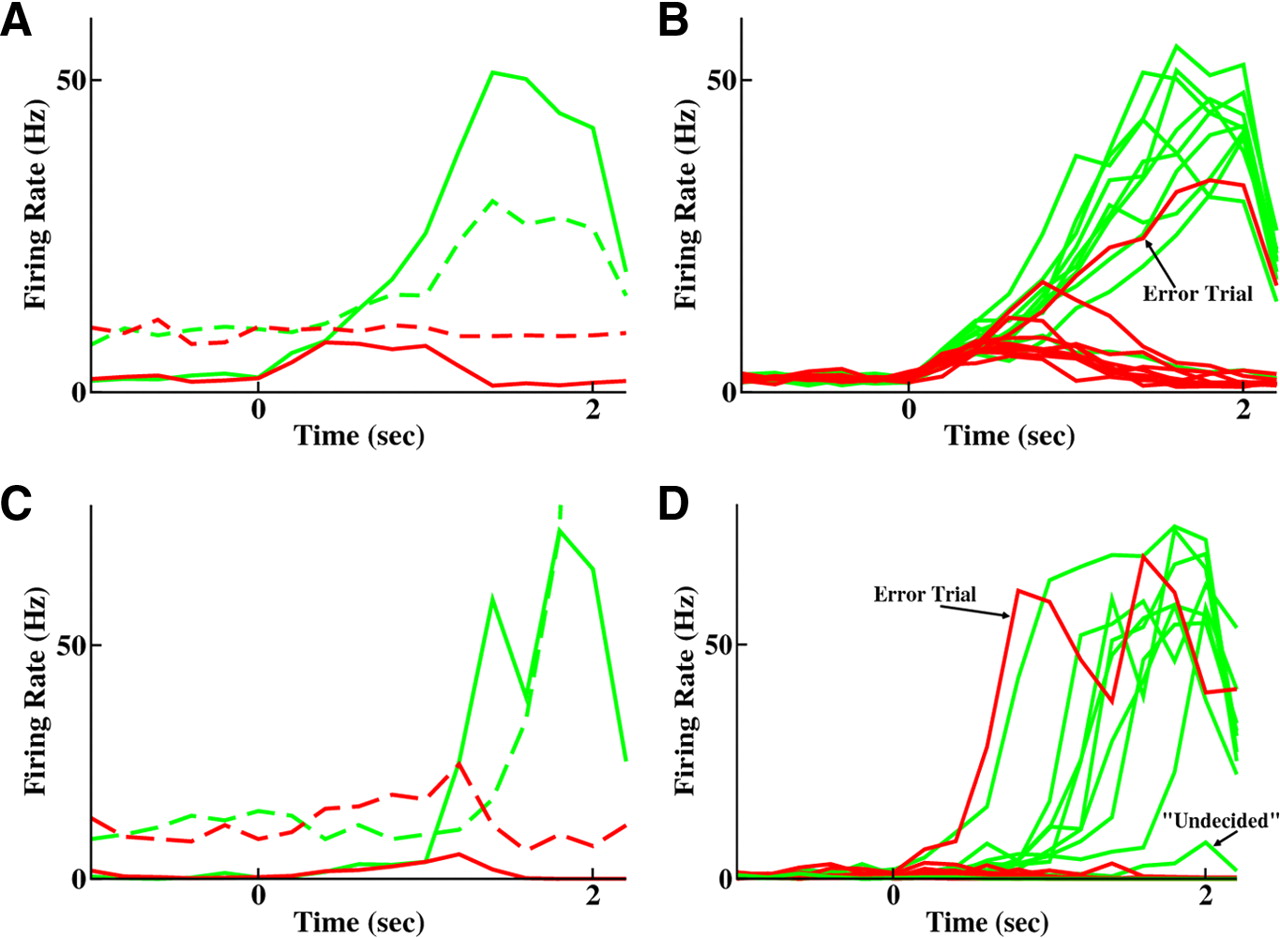
Decision-making network produces a winner-takes-all response to a small bias in input. A, B, Network in ramping integration mode (parameters of Fig. 5A,B). A, In a single trial, solid curves indicate activity of each excitatory population, and dashed curves indicate activity the inhibitory population of the corresponding color. B, Activity of the two excitatory populations across 10 trials, given a small bias current to the “choose swallow” population (green) over the “choose spit” population (red). An error trial is visible when the red curve reaches high activity. C, D, Network operating in jumping mode (parameters of Fig. 5C,D). C, A single trial with average activity of excitatory populations solid and their corresponding inhibitory population in the same color dashed. D, Ten trials of activity of the two excitatory populations given a small bias to the swallow population (green). An error trial is visible when the choose spit population (red) achieves high activity. On one trial, neither population reaches high activity, representing an undecided state.
HMM analysis of spike trains from eight representative cells selected in equal numbers from each pool reveals the difference in the two modes of operation (Fig. 5). Ramping produces slow transitions (153 ± 47 ms) between states and an extra HMM state of intermediate activity between spontaneous and persistent states (Fig. 5A,B). However, the jumping mode produces just two stable states with sharp transitions (mean of 19 ± 5 ms) between them, with highly variable timing of those transitions (Fig. 5C,D) (mean transition time of 1065 ± 556 ms).
The advantage of computer simulation is our ability to monitor every single neuron in every trial. Thus, we can analyze the fine temporal details of network activity on a trial-by-trial basis, in a manner not possible in a biological network. In particular, neurons that have similar responses (typically all 80 excitatory neurons or all 20 inhibitory neurons of a specific population in our simulations) can be binned together, reducing noise, and allowing us to obtain the dynamics of each type of neuron during each trial. To reduce measurement noise, the bins we use to calculate mean population activity on a trial-by-trial basis are significantly larger (200 ms) than the 2 ms bins used as input to the HMM analysis.
Figure 6, A and C, shows the mean activity of the four types of cell: excitatory in solid line, inhibitory in dashed lines, with the pool receiving more input in green and the pool with less input in red. The slower ramping on a single trial is apparent in Figure 6A, with the network in ramping mode, compared with Figure 6C, with the network in jumping mode. Activities of the excitatory pools across 10 trials are shown in Figure 6, B and D, respectively, for ramping and jumping modes of decision-making. These panels each include an “error trial” (in red), during which the population with less bias became the highly active one. Figure 6D shows, in addition, a trial in which neither pool made the transition to the active state within the allocated 2 s of stimulus response. Such trials, which we label as “undecided” and count as ½ for a correct trial and ½ for an error trial, disappear if response time is drawn out far beyond 2 s. Although noise does lead to variability across trials in neural responses in the ramping mode (Fig. 6B), the latency variability is significantly greater in jumping mode (Fig. 6D).
To quantify these differences in transition speeds, we defined the onset time of a firing rate change as the point at which mean population activity passed 5 Hz (a rate never produced in the spontaneous state) and calculated how long it took increasing firing rates to reach an arbitrary threshold of 40 Hz. In ramping mode, firing rate changes commenced at 240 ± 84 ms (mean ± SD), whereas in jumping mode, firing rate changes commenced at 820 ± 416 ms (mean ± SD). This fivefold difference in SDs reflects the fact that ramping begins at approximately the same time on each trial, whereas jump times evince trial-to-trial variability. Mean time to reach 40 Hz in ramping mode is 1400 ms, whereas in jumping mode this change took only 460 ms; jumps were swift, whereas ramps were slow. The variability in the rate of slow deterministic ramping (Fig. 6B) is primarily responsible for the trial-to-trial variability in the time taken to reach 40 Hz (SD of 246 ms) in ramping mode. However, in jumping mode, the SD of jump onset time entirely accounts for the SD of the time taken to reach 40 Hz (434 ms), a fact that demonstrates that jumps were also much more reliable in duration than ramps.
Note that the transitions in jumping mode of our model were much slower than transition times found by HMM analysis of the same data for two reasons. First, population activity is binned at 200 ms, limiting our ability to resolve rate of change, whereas HMM analysis can use 2 ms bins. Second, in our sparse random networks, neurons within a population differ in their inputs and excitability, so the times for the average rate of 80 cells to increase is much longer than the times for the rate of individual cells to change.
To further analyze the behavior of our model network, we switch between modes of decision-making by adjusting, in a single network, the stability of the spontaneous state of activity of the two excitatory populations when an input is present. In the jumping mode, the spontaneous state is stable, either because both populations receive relatively little total input (Fig. 7A) or because we globally increase the leak conductance of all cells (Fig. 7B) to represent a constant inhibitory drive. Figure 7A shows the results of a speed–accuracy tradeoff within the jumping mode. As we enhance the stability of the spontaneous state (i.e., reducing the total applied current and moving along the x-axis to the left), the probability increases that the decision-making network response will follow input bias. Thus, performance improves with increased stability of the spontaneous state. However, in the case of highest stability and best performance, the time taken to produce a decision was frequently >10 s, far longer than of behavioral relevance for taste processing. That is, in the jumping mode, any increase in performance comes at the cost of increased decision-making time (see Analyses in the supplemental data, available at www.jneurosci.org as supplemental material). In the ramping mode at larger applied currents, meanwhile, choice probability is approximately constant, such that there is no benefit of increasing integration time.

Benefits and limits of noise and the stochastic, jumping mode of decision-making in a fixed time interval. A, Total applied current is varied to shift the network from the ramping mode (high total applied current) to the jumping mode of decision-making (low total applied current) while maintaining a fixed bias (difference between the currents to the two populations is held fixed). Proportion of trials in which the winning pool is the one with greater input, maximized when the system is in jumping mode. B, With constant inputs for a limited, 2 s decision-making period, inhibitory conductance is increased to shift the network to jumping mode. Optimal performance occurs in the parameter region of the jumping mode. Bottom curve, Inputs are fixed currents. Top curve, Inputs are Poisson spike trains with the same mean current as the bottom curve. Note that performance is better when inputs are noisy. C, Performance varies with size of network, always improving with network size (which reduces internal noise) for deterministic integration in the ramping mode but having an optimal level for the jumping mode. Note that noise is uncorrelated across cells in these simulations, so unrealistically low levels of internal variability could be reached with large network size.
We define performance as the difference between percentage of “correct” trials and “incorrect” trials, so that chance response corresponds to zero performance. Our definition of performance penalizes those undecided trials in the jumping mode when no transition away from spontaneous activity was made during stimulus presentation, by assuming no better than chance responses on such trials, thus neglecting any information from the inputs that could affect any forced response. Such undecided trials, when all cells remained at or near spontaneous activity levels, never occur in the ramping mode: in all ramping trials, at least one population reached activity at least 20 Hz higher than the other for two consecutive 200 ms time bins (our criterion to select the “winning” population) so a binary response could be determined even if the attractor state was not yet reached.
When we restricted the duration of stimulus processing to 2 s [a typical time for a taste to remain on the tongue before swallowing (Travers and Norgren, 1986)], performance was best (Fig. 7B) when the spontaneous activity is stabilized by an increase of inhibitory current to all excitatory cells in the network. The peak in performance occurs, furthermore, when this inhibitory current drives the network into the jumping mode of decision-making. At even higher levels of inhibition, the network more frequently remains in the spontaneous state, producing no decision within the stimulus duration of 2 s, and thus overall performance declines. Such a peak in performance, in which the timescale for a noise-dependent state transition approaches but does not exceed the timescale of the input (in our case the duration of the input), is an indication that our system undergoes stochastic resonance (McDonnell and Abbott, 2009).
Addition of noise to the stimulus, produced when inputs are simulated as Poisson spike trains rather than as constant currents, has little effect in the ramping mode, because the difference in the two inputs producing a bias for deterministic integration is of a far greater magnitude than the fluctuations in the inputs. Such inclusion of input noise allows the network to operate farther into the region of stochastic transitions in its jumping mode, however, specifically because increased noise increases the likelihood of a state transition before 2 s (Fig. 7B). Thus, although stimulus noise inevitably reduces the reliability of the difference between two stimuli, it paradoxically leads to better performance in the jumping mode by accelerating the decision-making process.
The benefit of the jumping mode for decision-making—an improved ability to produce a binary output that follows a small bias—arises because the decision-making network has its own internal noise. To explore the extent of the advantage of the jumping mode over the ramping mode, we can reduce the effect of internal noise simply by increasing the number of neurons in each network pool (and simultaneously scaling down individual synaptic strengths); this reduces noise because the noise is injected into each neuron independently. Performance of the jumping mode peaks at a level of 50 independent cells (Fig. 7C): increasing noise heightens the probability of errors, whereas reducing noise lessens the ability of the network to respond in the stimulus window. However, the advantage over the ramping mode remains across a realistic range of levels of network noise [up to a noise level corresponding to 100 independent neurons, beyond which in vivo correlations render any additional averaging out of noise impossible (Zohary et al., 1994)]. Ultimately, deterministic integration in the ramping mode performs better only under conditions in which internal noise levels are reduced further (as they can be in computer simulations, in contrast to in vivo): a jumping network performing stochastic transitions under low-noise conditions ultimately reaches zero performance, because no transitions occur in the absence of noise, whereas such noise is only a detriment to the performance of a ramping network performing deterministic integration.
To explore the generality of these findings, in Figure 8 we present the results of parameter exploration in which, compared with Figure 7B, the signal is stronger, because the input rates are either doubled (Fig. 8A–C) or quintupled (Fig. 8D–F). The network is slightly altered from that of Figure 7 in an attempt to optimize the ramping mode; we reduced the recurrent excitation within a pool to reduce the speed of deterministic transitions. In all figures, the transition from ramping to jumping arises as we increase leak conductance to stabilize the spontaneous state; the stabilization requires higher leak conductance with greater external inputs. The transition is obtained by monitoring the SD of transition times as the network size is increased to reduce internal noise. In the ramping mode, the reduction of noise reduces SD of transition times, but in the jumping mode the opposite occurs (i.e., because of the increase in mean transition time, a reduction in noise increases absolute temporal variability).

Optimal mode for decision-making shifts to ramping with strong external signal, low internal noise, and short duration of stimuli. A–C, Response of the network with a doubling of both inputs used in Figure 7, B and C. Network size increases from left to right panels: A, n = 50; B, n = 100; C, n = 200. D–F, Response of the network with a factor of 5 increase in both inputs of Figure 7, B and C. Network size increases from left to right panels: A, n = 50; B, n = 100; C, n = 200. In A–F, input durations are 1 s (red), 2 s (green), or 5 s (blue). The transition between jumping and ramping modes is determined by a switch from increasing to decreasing variance of response times with reduced internal noise (larger networks).
In Figure 8A–C, we see for all three population sizes (50, 100, and 200) and for all three stimulus durations (1, 2, and 5 s) that optimal performance occurs with sufficient leak conductance that the system operates in jumping mode. However, a dramatic drop off in performance occurs when the leak conductance is increased beyond that needed for optimal performance, because the response time rises extremely rapidly (supplemental data, available at www.jneurosci.org as supplemental material) with additional stabilization of the spontaneous state. A fivefold increase of the inputs from our base conditions produces a different story (Fig. 8D–F). In all cases but one, optimal performance arises either in the ramping mode or on the boundary of ramping and jumping modes. Only in the system with highest internal noise (50 cells with independent noise, per group) and longest stimulus duration (5 s) is the jumping mode still optimal. Thus, in general, we find that a strong signal (here an average of an extra 50 spikes/s through 5 nS AMPA receptor-mediated synapses to each excitatory cell of the biased population) favors the deterministic ramping mode, whereas high internal noise (equivalent to 100 or fewer cells with independent Poisson-like firing per population) combined with a long allowed response time favors the jumping mode.
One factor that can have a deleterious effect on the response is variability in the network preceding stimulus onset. In fact, even if the spontaneous state is deterministically stable, in principle, spontaneous transitions can produce a random response (Miller and Wang, 2006). In Figure 9 we assess, using a firing rate model and nullcline analysis, how variation in starting conditions can produce differing responses once the stimulus is present. The nullclines (Fig. 9, S-shaped curves) indicate the values at which the rate of change of one variable is 0 given a fixed value of a second variable. In this case, the two variables are the synaptic outputs of the two excitatory populations, which are monotonic functions of the firing rate of each population. The green curve shows where dS2/dt = 0 at fixed S1, and the red curve shows where dS1/dt = 0 at fixed S2. The S-shape to each curve indicates that one population is bistable (can have both a stable low firing rate and a stable high firing rate) for a small range of activity of the other population. Intersections of the two nullclines indicate fixed points of the system, which we mark by filled circles for stable states and open circles for unstable states.

Nullcline analysis reveals how the jumping mode reduces response variability arising from non-identical initial conditions. Nullclines in the synaptic variables indicate the steady states of the system. Green lines indicate dS1/dt = 0 for a given S2; red lines indicate dS2/dt = 0 for a given S1. Filled circles are stable fixed points of the system, and open circles are unstable fixed points. Trajectories for the system with inputs biased by 10% in favor of S2 from a symmetric range of starting points are presented without noise (A–C) and with noise (D–F). Orange trajectories result in a correct response with high S2, low S1; magenta trajectories show an incorrect response with low S2, high S1; blue trajectories result in a lack of response with low S1 and S2. A–D, With inputs of 0.0040 and 0.0044, the low activity state is stable; B–E, with inputs of 0.0050 and 0.0055, the low activity state is just unstable and noise generates many errors; C–F, with inputs of 0.0200 and 0.0220, the low activity state is highly unstable and asymmetry in the initial state of the system produces multiple errors.
In Figure 9A–C, we increase the input strengths multiplicatively, thus increasing the signal, to switch from jumping mode (Fig. 9A) to a slow ramping mode via 25% increase of inputs (Fig. 9B) and a strongly ramping mode with fivefold increase of inputs (Fig. 9C). The 10% bias of inputs favors the fixed point (filled circle) with high S2 and low S1. In the absence of noise, all trajectories (blue) in the jumping mode (Fig. 9A) terminate in the symmetric state with low S1 and low S2, whereas in the deterministic ramping mode (Fig. 9B), 10 of 11 trajectories (orange) terminate in the state with high S2 (near perfect performance). However, with even stronger signal (Fig. 9C), a large number of errors occur, because many initial conditions produce a trajectory (in magenta) that terminates with large S1 and low S2 (only 8 of 13 trajectories follow the input bias).
Figure 9D–F shows the same nullclines as Figure 9A–C, with the same set of initial conditions but with a small amount of noise added to the trajectories. The noise enables the jumping mode to produce responses (Fig. 9D) so that 10 trajectories terminate at high S2 versus one at high S1 (and 2 at low S1, low S2). The noise produces more errors in the slow ramping mode so that eight trajectories terminate at high S2 and 5 at high S1, whereas trajectories in the strong, fast ramping mode are little affected by the additional noise (Fig. 9F).
The benefit of a high threshold in the jumping mode for stochastic decision-making can be appreciated by considering two Gaussian distributions of instantaneous input current, with a difference in means, D, and SDs, σ. Rather than integrating the instantaneous current over time to distinguish the two distributions, one could set a threshold current, T, and ask the following: what is the probability that one distribution of inputs might produce an instantaneous current above that threshold compared with the other distribution? That is, we assume that a superthreshold instantaneous current is sufficient to cause a jump to one of the two decision states. Measuring T with respect to the mean current of the two distributions, we thus compare the ratio of
In summary, a small increase in the stability of the initial state beyond its optimum can easily lead to a network with prohibitively high response times. However, maintaining stability of the initial state on stimulus onset has clear advantages (Fig. 9). Together, these two results lend theoretical support to the concept of an urgency signal (Cisek et al., 2009)—in our case, a gradual ramping up of global excitation or ramping down of global inhibition—to optimize decision-making within the jumping mode.
Discussion
The variability and apparent unreliability of individual neural spikes, particularly notable in awake animals (Shadlen and Newsome, 1994, 1998; Zohary et al., 1994), long ago led researchers to begin averaging neural spike trains across multiple trials to obtain reliable data. This practice is now ubiquitous, although we have entered an era when multiple cells are recorded simultaneously on a regular basis, making such across-trial averaging less essential. However, in the absence of a good reason to suppose that across-trial averaging is missing any important aspect of the data, such traditional methods, being easy to use and explain, will continue to be the norm. In this paper, we describe a jumping mode of network operation that is obscured by across-trial averaging but that matches the trial-to-trial variability in cortical neural activity during sensory processing observed through Hidden Markov modeling (Abeles et al., 1995; Seidemann et al., 1996; Jones et al., 2007). Furthermore, we reveal a useful computational aspect of this mode of operation in decision-making, expanding theoretical work by others in this area (Deco and Romo, 2008; Mart í et al., 2008; Deco et al., 2009).
We do not attempt here to reproduce all the specific details of neuronal responses during taste processing (nor do we reproduce the entire system responsible for such responses). We do, however, show how some important key response features arise, features that may also be important in other functions of cortical activity. First, we demonstrate how neurons possessing only fast time constants (the slowest time constant in our simulations is that of NMDA receptor activation, lasting 100 ms) can produce time structure that is an order of magnitude longer, even in the presence of a constant, time-invariant stimulus. The ability to remain in one constant state for this long allows completion of one stage of processing (such as taste identification) before the next stage (deciding on a behavioral response) commences. This “slowing” of cortical processing suggests a mechanism that can explain a wide range of behavioral responses, some with relatively slow reaction times, in a unified manner (Halpern, 2005).
Second, we show that stable states of activity can transition rapidly to other states, at latencies that vary from trial to trial. The trial-to-trial variability of transition times is produced because of the inherent noise in the network. Others (Moreno-Bote et al., 2007) have considered similar state transitions as the basis for binocular rivalry in visual perception and have shown that the distribution of times between transitions can be used to elucidate more detailed biophysical properties of the cells and network connections. This analysis has the potential to explain both the reliability and “trial-to-trial” variability of perceptual judgments (Deco et al., 2007a,b, 2009; Deco and Romo, 2008), again within a single unified framework: that is, the same mechanism that drives the system through states is responsible for the “random” variability in response speed. Our framework may also be applicable to other systems in which sequences of activity states have been observed, such as during songbird singing (Fee et al., 2004; Hampton et al., 2009) and insect olfaction (Laurent et al., 2001).
Previous models of decision-making have assumed the existence of a perfect integrator, so that integration of evidence follows a biased random walk (Ratcliff et al., 1999, 2007; Smith and Ratcliff, 2004; Ratcliff and McKoon, 2008). In these models, a constant bias in the inputs produces a constant ramping up of activity of an appropriate set of cells as a function of time; trial-to-trial fluctuations represent random noise distributed about a mean ramping rate. Other models, based on the properties of connected groups of neurons, have shown that such gradual ramping and accumulation of evidence can arise in an attractor model (Wang, 2002; Wong and Wang, 2006; Wong et al., 2007; Wong and Huk, 2008), without the need for a perfect integrator. However, all models that produce a slow time constant for deterministic integration require a level of fine tuning (Seung, 1996; Aksay et al., 2000; Seung et al., 2000a,b) that may be difficult to realize biologically.
Our model is a variant of such an attractor model, operating in a regimen in which deterministic integration is impossible, so fluctuations are key (Deco et al., 2007b). In such a regimen, fine tuning is not as necessary (Koulakov et al., 2002; Goldman et al., 2003; Okamoto and Fukai, 2003). The discrete jumps in activity that occur in any individual trial resemble a gradual ramping of activity when neural data is averaged across trials (Okamoto and Fukai, 2001), but in our model, this ramp is artifactual. In particular, trial-to-trial variability in timing of sharp transitions, and a gradual ramping of activity on each trial, will look similar in any analyses that average across trials (cf. Deco et al., 2005).
Such an effect has been observed in a number of systems (Abeles et al., 1995; Seidemann et al., 1996; Jones et al., 2007) and has been suggested, following single-unit analysis, to characterize cortical activity during delay-period “ramping activity” in the anterior cingulate cortex of monkeys (Okamoto et al., 2007). In most cases, recognition of such a process requires the use of HMM (or similar analyses) brought to bear on simultaneously recorded multi-electrode data, although not necessarily dense multi-electrode data: both times HMM have been applied successfully to neural data (Seidemann et al., 1996; Jones et al., 2007), a handful (6–12) of neurons have been enough to allow reliable detection of states. The use of more neurons might reveal greater complexity (subsets of neurons performing independent sequences of states, for instance), but it is clear that these dynamical processes are not sparse: whereas many neurons work together during stimulus processing, the patterns that reflect this processing can be observed in >50% of the neurons (Jones et al., 2007) and thus in relatively small recorded ensembles.
A significant theoretical difference between the two modes of operation of an attractor-based decision-making network has to do with the fact that, in the jumping mode, the initial, spontaneous state of activity is deterministically stable even while the inputs are present. Maintaining the deterministic stability of the initial activity state can allow the network to more reliably follow a small bias of the inputs than is possible in a ramping mode when the initial state is unstable and a response is deterministically “forced”. This benefit is apparent when a major cause of errors in the ramping mode of decision-making arises from variability in network activity before and up to the moment of stimulus onset. Such variability in initial conditions has less effect when the spontaneous state remains stable, and thus a source of error is greatly reduced (Fig. 9).
Of course, the higher the threshold for a decision, the more stable is the initial state and the longer it takes to generate a response; this produces the well known tradeoff between response speed and accuracy (Ratcliff, 1985; Ratcliff and Smith, 2004; Smith and Ratcliff, 2004; Shea-Brown et al., 2008; Eckhoff et al., 2009) (also see the analyses in the supplemental data, available at www.jneurosci.org as supplemental material). If a finite decision time is needed, such a tradeoff leads to an optimal level of stability for the initial state. Similarly, for a fixed network with a stable initial state, an optimal level of noise is needed to balance the desire for a timely transition during the response time with the need to keep any input bias from being hidden in the variability. Such a matching, of the timescale of transitions produced by noise to the timescale of a stimulus to produce optimal performance, is a hallmark of stochastic resonance (Gammaitoni et al., 1998; McDonnell and Abbott, 2009).
Because the addition of noise can increase the speed with which a network jumping mode processes input, we find our simulation capable of performing an unlikely feat: the addition of a certain amount of noise to the inputs of the network allows the network to more reliably detect a difference between the inputs. The optimal level of stimulus noise will depend on the level of internal network noise (and vice versa). In the brain, inputs to one region from another contain inherent variability and fluctuations but so too do environmental stimuli. The improved performance of our network with stochastic inputs leads to the suggestion that the brain can use environmental fluctuations to enhance its function (Deco et al., 2009).
Footnotes
This work was supported by National Institutes of Health/National Institute on Deafness and Other Communication Disorders Grants R01DC00945 (under the National Science Foundation/National Institutes of Health Collaborative Research in Computational Neuroscience mechanism) and R01DC007708 and the Swartz Foundation.
- Correspondence should be addressed to Paul Miller, MS013, Volen Center for Complex Systems, Brandeis University, 415 South Street, Waltham, MA 02454-9110. pmiller{at}brandeis.edu


