

Abstract
Neurons in macaque primary visual cortex (V1) show a diversity of orientation tuning properties, exhibiting a broad distribution of tuning width, baseline activity, peak response, and circular variance (CV). Here, we studied how the different tuning features affect the performance of these cells in discriminating between stimuli with different orientations. Previous studies of the orientation discrimination power of neurons in V1 focused on resolving two nearby orientations close to the psychophysical threshold of orientation discrimination. Here, we developed a theoretical framework, the information tuning curve, that measures the discrimination power of cells as a function of the orientation difference, δθ, of the two stimuli. This tuning curve also represents the mutual information between the neuronal responses and the stimulus orientation. We studied theoretically the dependence of the information tuning curve on the orientation tuning width, baseline, and peak responses. Of main interest is the finding that narrow orientation tuning is not necessarily optimal for all angular discrimination tasks. Instead, the optimal tuning width depends linearly onδθ. We applied our theory to study the discrimination performance of a population of 490 neurons in macaque V1. We found that a significant fraction of the neuronal population exhibits favorable tuning properties for large δθ. We also studied how the discrimination capability of neurons is distributed and compared several other measures of the orientation tuning such as CV with Chernoff distances for normalized tuning curves.
- primary visual cortex
- orientation selectivity
- population coding
- macaque monkey
- Chernoff distance
- discrimination
Introduction
Neurons in primary visual cortex (V1) are selective for the movement direction or the orientation of line-like simple visual patterns. The shape of the response tuning curve and orientation selectivity of neurons in macaque V1 are diverse (Ringach et al., 2002). Our motivation was to understand the possible functional use of the observed diversity in V1 orientation tuning.
The orientation selectivity of neurons in V1 has been studied mainly in two different ways. First, the most informative point of a tuning curve, which is usually the steep flank part of the tuning curve, is selected, and discrimination capability of the neuron for two angles is computed using ROC analysis or neurometric functions (Bradley et al., 1987; Hawken and Parker, 1990; Vogels and Orban, 1990; Parker and Newsome, 1998). But these studies only analyzed discrimination for two nearby angles and did not clarify the functional use of broadly tuned neurons. In addition, discrimination capability computed in this way depends only on the local shape of the tuning curve. The advantage of having diversity in the global shape of tuning curves may be clear only in terms of population coding.
Discrimination capability of a population of neurons is more difficult to study mainly because a practical measure for it has been lacking. In several studies (Seung and Sompolinsky, 1993; Abbott and Dayan, 1999; Sompolinsky et al., 2001), Fisher information was used to study population coding. But Fisher information can be used only when angles are very near to each other. Other well known measures such as mutual information are computationally too expensive to calculate for a population of neurons.
Here, we studied the relationship between the shape of a tuning curve and the discrimination capability of a population of neurons using the Chernoff distance (Cover and Thomas, 1991; Kang and Sompolinsky, 2001). The Chernoff distance is a measure of the difference between two probability distributions and has direct relationships with other information measures such as Fisher information, mutual information, and the error of maximum likelihood discrimination.
For a population of neurons with preferred orientations that are distributed isotropically, the Chernoff distance between two distributions of spike counts corresponding to two different orientations depends on only δθ, the difference in the orientations. The information tuning curve is a plot of Chernoff distance as a function of δθ. The shape of the information tuning curve characterizes how different orientations are represented by the activities of a population of neurons. In Results, we studied how the information tuning curve depends on various features of the response tuning curve.
We applied the theoretical analysis to macaque V1 data. The results suggest that diversity may exist in V1 because different neurons are optimal for different discrimination tasks. It also shows that neurons in macaque V1 are not optimized for the discrimination of nearby angles. Finally, we discussed the relationship between Chernoff distance and several other measures of orientation tuning such as circular variance (CV) and tuning width.
Materials and Methods
Preparation and recording. Acute experiments were performed on 40 adult Old World monkeys (Macaca fascicularis) in the laboratories of R. M. Shapley, M. J. Hawken, and D. L. Ringach and colleagues (cf. Ringach et al. 2002). The methods of preparation and single-cell recording are the same as those described by Ringach et al. (2002). Each cell was stimulated monocularly via the dominant eye and characterized by measuring its steady-state response to drifting sinusoidal gratings (the non-dominant eye was occluded). With this method, basic attributes of the cell, including spatial and temporal frequency tuning, orientation tuning, contrast response function, and color sensitivity, as well as area, length, and width tuning curves, were measured. Orientation tuning curves were measured at high contrast (0.8). Spike times were recorded for 18 directions (every 20°). Spatial frequency, temporal frequency, and size of the sinusoidal gratings were optimized for each cell separately to maximize the peak response.
A model for the directional tuning of the spike count. We introduced a Gaussian model for the directional tuning of mean spike count and fit the model to the measured mean spike counts for 18 directions to reduce noise in the experimental data and to extract a small number of parameters to describe the shape of the tuning curve. The model tuning curve λ(θ) is described in Equation 1:  (1) where θ′ = R(θ, θ0) and θ″ = R(θ, θ0 + π). θ0 is the preferred direction of the neuron. R(x, y) = min{|x – y|, 2π – |x – y|} is the angle between x and y. See Figure 2 for examples of tuning curves. For each neuron in the V1 data, we minimized the squared error, Er(A, B1, B2, σ, θ0):
  (2) where m(θi) is the mean spike counts of the neuron for the direction, θi. We also defined the error ratio, RER to measure the goodness of the fit to a Gaussian model:
  (3) where
  and m0 is the mean of m(θi). A*, B1*, B2*, σ* and θ0* are the values of parameters minimizing the error Er(A, B1, B2, σ, θ0).

The response tuning curves of six neurons in V1. Solid lines are models of tuning curves fitted to experimental results. Filled dots present the observed mean spike counts for 1 sec.
In this study, we ruled out neurons with a maximum firing rate lower than five spikes per second. Seventy-six neurons among 897 neurons were discarded in this way. We fitted the observed mean spike counts to our Gaussian model (see Eq. 1) and did not study further those neurons that did not show a good fit to the proposed model (RER > 0.3). Three hundred thirty-one neurons among 821 neurons are discarded in this way. The total number of neurons in the resulting database was 490. Most of the discarded neurons should be considered as “noninformative” in any sense. For most of the discarded neurons, the tuning curves were very irregular, and baseline firing rates were relatively large. Spiking activities of those neurons were less reliable so that the statistics of the spike count had larger variance. For a few neurons (<1%), our model was bad because the distance between the peaks of the tuning curve was different from π. But such neurons were rare and ignored in this study.
Classification of neurons. Neurons are classified into orientation-selective (OS) neurons and direction-selective (DS) neurons based on the ratio of the heights of two peaks of tuning curves RB. RB is min(B1, B2)/max(B1, B2) where B1 and B2 are the height of two peaks (see Eq. 1 and Fig. 4). RB is a ratio of the responses for the preferred direction and the opposite direction. For tuning curves of ideal OS neurons, RB is 1, and for ideal DS tuning curves, RB is 0. We classified neurons as OS if RB > 0.5 or as DS otherwise. We found that 240 neurons are OS and 250 neurons are DS among 490 neurons. A similar method was used in a previous study (Hawken et al., 1988).

A model of tuning curve λ(θ). λ(θ) = A + B1 exp(–θ′2/2σ2) + B2 exp(–θ″2/2σ2). θ′ (θ″) is the angle between θ and 90° (270°). For this example, A = 5, B1 = B2 = 20 σ = 22.5°.
Spike count statistics. As for the statistics of the spike count, we assumed that it follows a Poisson distribution, the mean of which is the same as the variance. It is observed in experiments that the variance is often approximately proportional to mean spike count (Tolhurst et al., 1983). Real distributions show some deviations from Poisson distributions. Figure 1 shows a scatter plot of the mean and the variance of spike count at the preferred orientation for 490 neurons. Here, we just assumed Poisson distributions and focused on studying the role of the shape of tuning curves in the neuronal representation of sensory information.

Mean and variance of spike counts of 490 neurons for preferred directions of each neuron. For each neuron, the number of spikes for one period of sinusoidal grating stimulus was counted. The average value of the ratio of variance and the mean is 1.9, but the distribution of the ratio between mean and variance has a peak at 1, which is the value for Poisson distributions.
Significance of correlation. We calculated correlation coefficients between several features of tuning curves. To show the significance, we randomly shuffled the indices of one of two quantities with which the correlation coefficient is calculated and calculated the correlation coefficient again. We used the frequency that the absolute value of this correlation coefficient after random shuffling is larger than the absolute value of the correlation coefficient before random shuffling as a measure of the significance. We did this 1000 times. If none of the trials generated a correlation coefficient larger than the original, we took the significance as <0.1%.
Results
Distance measures in the representation space of a population of neurons
To study the relationship between the shape of a tuning curve and the capability to discriminate angles, a measure of discrimination capability should be defined and calculated. Here, we used Chernoff distance as a measure of orientation discrimination capability for a population of neurons.
Chernoff distance measures the difference between two distributions. For two distributions,  and
and  , Chernoff distance DC(θ1, θ2) is defined in the following way:
  (4)
(4)  (5) DC(θ1, θ2) is the maximum value of Dα(θ1, θ2) in terms of α within an interval 0 ≤ α ≤ 1. θi is the orientation of a sinusoidal grating, and
  is a vector of spike counts for a population of neurons.
  is the distribution of activity across the population
  when the stimulus with the orientation θi is presented.
  is a summation over all possible
  .
.
DC(θ1, θ2) ≥ 0 for any pairs of distributions. DC(θ1, θ2) is 0 if and only if two distributions are the same. DC(θ1, θ2) = DC(θ2, θ1) so that DC(θ1, θ2) is uniquely defined for a given pair of orientations (Cover and Thomas, 1991; Kang and Sompolinsky, 2001).
Before deriving the form of Chernoff distance for a population of neurons, we introduced its relationship with Euclidean distance and the error of maximum-likelihood discriminator to explain the meaning of the Chernoff distance. For the relationships with Fisher information and mutual information, see Appendix. We discuss the advantage of Chernoff distance later (see Discussion).
The relationship between Chernoff distance and Euclidean distance
A simple way to measure the difference between two distributions is to calculate Hellinger distance (Cam and Yang, 2000), which is the Euclidean distance between  :
:  (6) Chernoff distance DC is the maximum value of Dα in terms of α, and Dα often has its maximum at α = 0.5. In this case, DC has the following relationship with Hellinger distance:
  (7) Hellinger distance is a more intuitive measure than Chernoff distance and often gives a very good approximation of Chernoff distance through Equation 6 if Dα has its maximum near α = 0.5. In fact, for the population of neurons with orientation symmetry as considered later here, Dα has a maximum at α = 0.5 (see Appendix). So Chernoff distance and Hellinger distance have the above relationship here.
Relationship with the error of maximum-likelihood discriminator
Another way of measuring the difference between two distributions is to perform discrimination using a discriminator and calculate the error. If two distributions are well separated, the discrimination error is small. The error of maximum-likelihood discriminator provides an error of the optimal discriminator.
When DC(θ1, θ2) ≫ 1, the error of the maximum-likelihood discriminator PC has an exponential dependence on the Chernoff distance DC(θ1, θ2) (Kang and Sompolinsky, 2001):  (8) The error of the maximum-likelihood discriminator PC is defined in the following way:
  (9) where Θ(x) is 1 for x > 0 and 0 for x ≤ 0. Equation 8 shows that if the Chernoff distance DC(θ1, θ2) is larger than 1, discrimination between two stimuli can be done with small error.
Whether the condition of DC(θ1, θ2) ≫ 1 is satisfied or not depends on the size of the population, the size of the time interval, and the shape of tuning curves in general. For two far-away orientations, this condition will be satisfied in most cases. For two orientations very close to each other, this condition may not be satisfied for a population of neurons with small size. For example, for a population of ∼100 typical neurons in V1, time interval ∼100 msec and angles larger than a few degrees, the Chernoff distance for this population is typically of the order of 1 if not much larger than that. So the condition required for the relationships between Chernoff distance and other information measures are satisfied in physiologically plausible situations. Chernoff distance has exponential relationships with mutual information and the error of maximum-likelihood discriminator. So, in practice, it is enough for Chernoff distance to be 3–4 to show good convergence to its asymptotic behavior.
Chernoff distance for a population of neurons
Here, we calculated the Chernoff distance for a population of neurons to get a quantitative relationship between the shape of the tuning curve and the discrimination capability of a population of neurons. We assumed that each neuron observed in the experiment represents a population of neurons with tuning curves that have the same shape as the observed one but in which preferred directions are different. We calculated DC(θ1, θ2) for this population of neurons.
When the tuning curve of a neuron is λ(θ), we generate tuning curves for a population of neurons using the operation of rotation and reflection:  (10) where θk = 360° k/N, k = 0... N – 1 and a = 1 or2. k is an index for rotation of the tuning curve, and a is an index for its reflection. The number of neurons in this population is 2N.
For this population of neurons, the Chernoff distance in Equation 4 has the following form (see Appendix for the derivation):  (11) The summation in Equation 11 can be approximated by an integration for large N:
  (12) Equation 12 shows us how the shape of the tuning curve is related to the discrimination capability of a population of neurons. The Chernoff distance is an extensive quantity so that it is proportional to the size of the neuronal population. Here, this N will be assumed to be divided out so that the Chernoff distance will be Chernoff distance per neuron in the population. DC(θ1, θ2) will be also written as DC(δθ) because DC(θ1, θ2) depends on θ1 and θ2 only through δθ.
The information tuning curve
We introduced the information tuning curve, a plot of DC(δθ) as a function of δθ, and discussed what it shows. Then we studied how DC(δθ) depends on the features of a tuning curve.
Examples of information tuning curves
Figure 2 shows response tuning curves with various shapes. There are broad tuning curves and narrow tuning curves. There are neurons with large baselines and neurons with baselines at zero. Neuron (a) has a bigger peak response than neuron (b). In the previous section, we found the relationship between the shape of a tuning curve and discrimination capability (Eq. 12). Figure 3 shows DC(δθ) as a function of δθ and how the diversity in the shapes of response tuning curves affects the discrimination capabilities of neurons.

Plots of DC(δθ) (i.e., examples of information tuning curves). Response tuning curves of corresponding neurons are shown in Figure 2.
The information tuning curve shows how the distance between two orientations in the neuronal representation space changes as the angle between them, δθ, increases. Consider information tuning curves (a) and (e) in Figure 3. One thing very easy to notice in the shape of those information tuning curves is that OS tuning curves like (a) in Figure 2 have information tuning curves with two peaks whereas a DS tuning curve like (e) in Figure 2 has an information tuning curve with one peak. Figure 2a is an OS tuning curve so that it is not able to discriminate two opposite directions. It is represented by a minimum of DC(δθ) at δθ = 180° in Figure 3. Discrimination capability of an ideal DS neuron such as (e) in Figure 2 should be maximized for two opposite directions. It is represented by a maximum of the information tuning curve at δθ = 180° in Figure 3e. There are also information tuning curves between these two cases like Figure 3c.
The information tuning curve also enables us to compare the discrimination capability of neurons quantitatively. Consider (a) and (b) in Figure 3. The information tuning curves have similar shapes, but the overall scale is more than three times bigger for (b), which means that we need three times as many neurons like (a) as neurons like (b) to achieve the same discrimination power. This is because of the big baseline of the response tuning curve of (a) (Fig. 2). Because the spike count is Poisson, a large baseline means spike counts are more stochastic. In fact, the modulation of the tuning curve for (a) is bigger than for (b), suggesting that without a large baseline, neuron (a) should be the more informative neuron. Neurons (d) and (f) also have information tuning curves with similar shape and different overall scales. Neuron (d) has a discrimination capability about 40 times bigger than neuron (f).
Information tuning also shows which tuning curves are good for the discrimination of nearby angles or faraway angles. Consider the information tuning curves of (d) and (e) in Figure 3. For (d), DC(δθ) increases with a large slope as δθ increases from 0. For (e), the information tuning curve has a much smaller slope. For narrow response tuning curves like Fig. 2d, information tuning curves increase with large slopes as δθ increases from 0 and saturate soon. For broad response tuning curves like Figure 2e, information tuning curves increase with small slopes and do not saturate. This makes neurons with narrow response tuning curves have a discrimination capability larger for small δθ and smaller for large δθ than neurons with broad tuning curves.
Parameters to determine the Chernoff distance
Here, we study which features of tuning curves determine DC(δθ). Consider the model of tuning curve λ(θ) shown in Figure 4. λ(θ) has two peaks at opposite directions. A is the level of baseline. B1 and B2 are the size of Gaussian peaks on the top of the baseline. σ is the width of the Gaussian functions. For simplicity, we considered only the case of OS tuning curves (B1 = B2 = B) here.
Equation 12 shows that DC(δθ, A, B, σ) is MBDC(δθ, A/MB, B/MB, σ), where MB = A + B is the peak response of the tuning curve. Note that DC(δθ, A/MB, B/MB, σ) is the Chernoff distance for a normalized tuning curve, the peak response of which is 1 because A/MB + B/MB = 1. We found that it is convenient to factor out the peak response MB and study how Chernoff distance depends on the remaining parameters because once we understand how DC(δθ, A/MB, B/MB, σ) behaves, it is easy to see how the original Chernoff distance depends on the peak response MB: it is proportional to MB. For this reason, we factored out peak response MB and studied how DC(δθ) depends on three parameters: δθ, relative baseline RA = A/MB, and tuning width σ. Relative baseline RA = A/MB is also the ratio of the responses to preferred orientation and orthogonal orientation (Gegenfurtner et al., 1996) and has been considered as a measure of orientation selectivity.
Dependence on the relative baseline RA
DC(δθ) decreases monotonically as RA increases because RA is a nontuned component of the tuning curve. Figure 5 shows a two-dimensional plot DC(δθ, RA, σ) for σ = 17.2°, a typical value of σ for neurons in V1. For RA as large as 0.5, DC(δθ) is already very small for all δθ. Also note that DC(δθ) for large RA looks flatter than DC(δθ) for small RA. This point is more clearly shown by the inset in Figure 5. DC(δθ) decreases monotonically as RA increases and decreases faster for larger δθ.

A surface plot of DC(δθ) as a function of RA andδθ.σ = 17.2°. The inset has plots of DC(3°) and DC(10°) as a function of RA. The solid line is for DC(3°). The dashed line is for DC(10°).
To study these points more quantitatively, we use the “half-width” value of RA, AH, where DC(δθ, RA = AH, σ) is DC(δθ, RA = 0, σ)/2. AH measures how fast DC(δθ) decreases as RA increases. If AH were small, it would mean DC(δθ) decays very fast as RA increases. If RA of a tuning curve were much larger than AH, the discrimination power of the tuning curve would be small, unless peak response MB were very big.
Figure 6 shows a plot of AH for several different values of σ and for all possible values of δθ. Note that DC(δθ) is very sensitive to RA. For RA as large as 0.15, DC(δθ) is already significantly smaller than DC(δθ) for RA = 0 because a typical value of AH is 0.1. AH is smaller than 0.142 and larger than 0.059 for any σ and δθ. These values of AH provide a scale for RA to be “too big” or “small enough.” For example, the response tuning curve of Figure 2a has too large a relative baseline because RA is about 0.5.

Plot of the half-width for relative baseline AH as a function of angular difference δθ. The dependence on tuning width is revealed by comparing these curves for tuning width σ = 11.5, 17.2, and 22.9°.
The effect of RA is not the same for different δθ. For small δθ, AH is 0.142 for any tuning width σ. Figure 6 shows that when δθ is close to 90° or 270°, AH tends to be smaller, which means that degradation of the discrimination capability is bigger for such δθ. This is the reason why DC(δθ) for large RA is flatter than for smaller RA as a function of δθ in Figure 5.
Dependence on tuning width σ
Consider the case that the relative baseline RA = 0. In this case, it is possible to calculate DC(δθ) analytically. Performing the integration in Equation 14 gives the following result:  (13) where R(x, y) is the angle between x and y.
As a function of σ, DC(δθ) has a maximum at a nonzero value of σ. Figure 7 shows a surface plot of DC(δθ) as a function of σ and δθ. For small σ, exponential terms in Equation 13 are very small for nonzero δθ, and DC(δθ) rapidly saturates to 4Nσ as δθ increases [for another example see (d) in Fig. 3]. This makes DC(δθ) flat as a function of δθ. Figure 7 also shows that a very narrow tuning curve does not produce large DC(δθ) because DC(δθ) converges to a value proportional to σ as σ → 0. For larger σ, DC(δθ) has round shape. In this case, the 4Nσ factor is larger but the exponential terms in Equation 13 decrease DC(δθ).

A plot DC(δθ) as a function of tuning width σ and δθ. Relative baseline RA = 0.
For each δθ, there is an optimal tuning width maximizing DC(δθ). Maximization of Equation 13 gives this optimal width, σ*, which is proportional to δθ:  (14) where x* satisfies 1 – e–x* – 2x*e–x* = 0. We assumed that δθ ≪ π.
An optimal value is more important when DC(δθ) decreases rapidly as the difference between tuning width σ and optimal tuning width σ* increases. We defined σH to measure how fast DC(δθ) decreases as σ departs from σ*. It is defined in a way similar to AH, such that DC(δθ, RA, σH) = DC(δθ, RA, σ*)/2. There are two σH for a given δθ and RA. Because the optimal tuning width σ* is non-zero, DC(δθ) would be decreased if σ deviated from σ* either by increasing it or decreasing it.
DC(δθ) depends on σ more sensitively for smaller δθ. Analytical study of Equation 13 shows that |σ* – σH| is O(δθ) for small δθ, that is, smaller for smaller δθ. Figure 8 shows σH and σ* together for A = 0. It is clear that σH is closer to σ* for small δθ. It means that neurons with broad tuning curves have poor capability to discriminate two nearby angles because tuning width is very different from the optimal value for nearby angles and DC(δθ) depends on σ very sensitively. In contrast, for a large δθ, DC(δθ) depends on σ more weakly so that informative neurons do not need to have σ very close to σ*.

Half-width for tuning widthσ,σH, andσ*. Solid lines are forσH. The dashed line is for optimal tuning width σ*. Relative baseline RA = 0.
We now consider the more general case in which the relative baseline RA > 0. This cannot be calculated analytically but can be calculated numerically. Figure 9 shows DC(3°) and DC(45°) for various values of RA. These should be compared with the RA = 0 case in Figure 7.

Plots of DC(3°) and DC(45°) as functions of tuning width σ. Each line is for a different value of relative baseline RA. From top to bottom, RA = 0, 0.1, and 0.2, respectively.
DC(δθ) has non-zero and finite optimal widths, σ* for non-zero RA, too. A smaller value of σ decreases the number of neurons active for the stimuli making DC(δθ) smaller. But it also increases the slope of the tuning curve making DC(δθ) bigger. This competition of two effects results in the existence of an optimal σ to discriminate two orientations in general.
Optimal tuning width σ* is bigger for larger RA. There is a small shift of σ* peaks as RA goes from 0 to 0.3. Figure 10 shows σ* for various values of RA. This graph also shows the δθ dependence of the optimal tuning width σ*.

Optimal tuning width σ* for several different values of relative baseline RA.
Neurons in V1
Here, we studied how the features of tuning curves are distributed within the population of neurons in V1 of macaque monkeys. After that, we discussed the distribution of discrimination capability of neurons in V1.
Features of V1 tuning curves
We studied how the features of tuning curves are distributed in V1 separately for OS and DS neurons. Figure 11 shows histograms of peak responses, relative baselines, and response tuning widths for 240 OS neurons and 250 DS neurons.

Histograms of peak response MB, baseline RA, and response tuning widthσ for OS population (top graphs) and for DS population (bottom graphs). MB is A + max{B1, B2}. RA is A/MB, where A is the baseline of the tuning curve and MB is the peak response. See Figure 4 for the description of the model of the tuning curve.
Peak responses, MB = max{B1, B2} + A, to 80% contrast stimuli are <100 spikes/sec for most of the neurons in V1. The means of MB are 38.6 and 49.7 spikes/sec for OS neurons and DS neurons, respectively. Only 37 neurons among 490 neurons have peak response higher than 100 spikes/sec. Thirty-three neurons among them are DS neurons.
Figure 11 shows the histograms of relative baseline RA = A/MB, too. Remember that typical values of AH are between 0.059 and 0.142 (Fig. 4). AH gives us a scale to see whether there is a significant degradation of discrimination capability attributable to the baseline. Figure 11 shows that RA is smaller than these values for most neurons. It means for most neurons RA of the tuning curve is not too large to degrade discrimination capability. The mean of RA is bigger for the OS population than the DS population.
Finally, the histograms of tuning width σ show that the distributions of σ are broad or nearly flat within intervals of allowed values. σ cannot be much larger than 40° for OS neurons because two Gaussians overlap if the peaks of Gaussians are too broad. Only DS neurons with one peak can have σ as large as 60°. This gives an upper bound condition on the value of σ. There is also a lower bound for σ. Because our experiment was done only for 18 directions (every 20°), this resolution limitation requires that σ should be larger than 7°. If neurons with tuning width smaller than this existed, our estimation of tuning width would be an overestimation.
It should be emphasized that the tuning widths of neurons in V1 are not optimized for the discrimination of nearby angles. Equation 14 and Figure 10 show that the optimal tuning width σ* is about 0.3δθ. This means for δθ as large as 10°, σ* is only 3 or 4°. Such a small tuning width is hard to find, if not impossible, in macaque V1. As orientation discriminators, neurons in V1 are optimized for δθ larger than 20°.
Table 1 shows the means and median values of distributions shown in Figure 11. The features of tuning curves are not independent of each other. There seems to be several different types of tuning curves in the neuronal population such as narrow OS tuning curves with zero baselines or broad OS tuning curves with large relative baselines and large peak responses. This gives correlations between different features of tuning curves within the neuronal population. We calculated correlation coefficients between different features for the OS and the DS populations. Table 2 shows these correlation coefficients.
Mean and median values of relative baseline RA, peak response MB, and tuning width σ
Correlation coefficients between relative baseline RA, peak response MB, and tuning width σ
There are three significant correlations. For the OS population, the relative baseline RA showed a significant correlation with the peak response MB (correlation coefficient, 0.24.). So there is a tendency that OS neurons with a large peak response have a large baseline. The mean of peak responses for OS neurons with relative baseline RA > 0.2 (80 cells) is 47.8 spikes, whereas that for OS neurons with relative baseline RA < 0.2 (160 cells) is 34.0 spikes.
Another significant correlation is found between RA and σ in the OS population (correlation coefficient, 0.39). Many narrow tuning curves of OS neurons do not have a baseline. The mean of tuning width σ for OS neurons with relative baseline RA > 0.2 (80 cells) is 26.4°, whereas that for OS neurons with relative baseline RA < 0.2 (160 cells) is 20.0°.
The last significant correlation is between MB and σ in the DS population. DS neurons with large peak responses tend to have broad tuning curves. For example, the average tuning width of 33 DS neurons with MB > 100 spikes/sec is 34.2°. The mean of σ for the other 217 neurons is 23.4°.
Specialization of neurons to different tasks
Here, we studied specialization in V1. We showed in Equation 14 and Figure 9 that optimal tuning width is different for different δθ so that neurons with different tuning width may be specialized to discrimination between angles with different ranges of δθ.
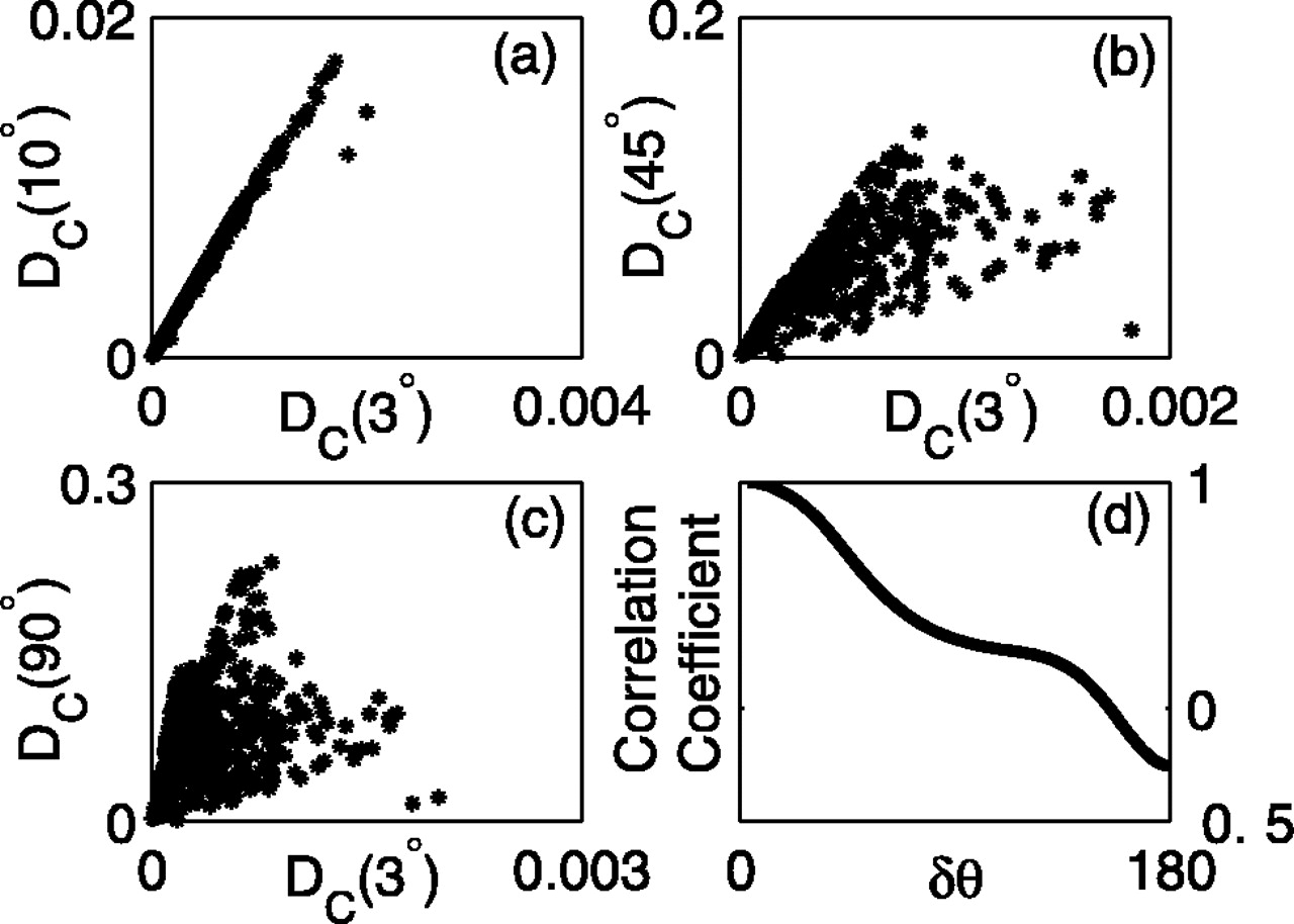
One way to study the specialization of neurons to different tasks is to compare the discrimination capability of neurons for two different angles. We made scatter plots of DC(δθ) for two different values of δθ for normalized tuning curves of 490 neurons. Figure 12 shows three scatter plots of DC(δθ1) and DC(δθ2) for δθ1 = 3° and δθ2 = 10, 45 and 90°, respectively. We can see that as δθ2 increases, the spread in the scatter plots increases.

Scatter plots of DC(δθ1) and DC(δθ2) for 490 neurons in V1. For the three scatter plots, δθ1 = 3° and δθ2 = 10, 45, and 90°, respectively. d is a plot of correlation coefficients between DC(3°) and DC(δθ) as a function of δθ.
We calculated the correlation coefficient between DC(3°) and DC(δθ) as a function of δθ. Figure 12d shows this correlation coefficient decreases almost linearly and becomes negative at δθ = 156°. This shows that neurons with large tuning widths do not have large discrimination capability for small δθ.
Comparison with other measures of orientation selectivity
Here, we compared Chernoff distance with several other measures of orientation selectivity such as CV (Swindale, 1998; Ringach et al., 2002), tuning width, and the ratio of the responses to preferred orientation and orthogonal orientation (Gegenfurtner et al., 1996). These measures were used as a measure of orientation selectivity without rigorous theoretical background. Here, we calculated each measure for 490 neurons and made scatterplots for various values of δθ. These measures weakly correlated with Chernoff distance in general because Chernoff distance is proportional to the overall scale of a tuning curve and the three measures we are comparing do not depend on it. It means what they measure should be orientation selectivity in terms of the shape of tuning curve ignoring overall scale. Therefore, we compared these measures with Chernoff distance after factoring out the peak response.
Comparison with CV and Chernoff distance
For a given orientation tuning curve λ(θ), CV is defined in the following way:  (15) fn is ∫dθeinθ λ(θ).
For a flat tuning curve, the CV is 1, and for a very narrow tuning curve with zero baseline, the CV is 0. Therefore, a bigger (smaller) CV is interpreted as a sign of lower (higher) orientation selectivity.
We found that the CV showed a very strong correlation with DC(δθ) when δθ is smaller than 90°. It has strongest correlation with DC(δθ) for δθ = 45°. Figure 13 shows three scatter plots between the CV and DC(δθ) for δθ = 3, 45, and 180°, respectively. The relationship between the CV and DC(δθ) is very linear.

Correlation between CV and DC(δθ). a–c are scatter plots for δθ = 3, 45, and 90°, respectively. d is a plot of correlation coefficients between RA and DC(δθ).
Our result shows that the CV is a good measure of orientation selectivity. But we also find that the CV behaves in a qualitatively opposite way to Chernoff distance sometimes. For example, we can calculate the CV and DC(δθ) for our model tuning curve shown in Figure 4. For one case, we fixed relative baseline RA to be 0 and changed σ from 8 to 40°. For another calculation, we fixed σ to be 20° and changed RA from 0 to 0.2. Figure 14 illustrates the results. Because the smaller CV (larger DC(δθ)) represents higher orientation selectivity, a plot of the CV and DC(δθ) should have a negative slope to be qualitatively correct. Figure 14 shows that, however, there are cases when the CV and DC(δθ) are positively correlated. When tuning width σ is small, the orientation selectivity for δθ = 90° increases, as we increase σ. The CV tells us, however, that orientation selectivity decreases. For smaller δθ, the part of line (a) with positive slope is shorter so that this problem disappears. When σ is fixed to be 20° and RA is changed, the line of the CV and DC(90°) has a negative slope.

Plot of CV and DC(90°). For the model of tuning curve, see Figure 4. For line (a), relative baseline RA = 0 and tuning widthσ is from 8 to 40° (left side is for smallerσ). For line (b), σ is 20°, and RA is from 0 to 0.2 (left side is for smaller RA).
Relative baseline and tuning width
In a previous section, we showed how DC(δθ) depends on RA and σ for idealized OS tuning curves. Here, we show correlations between DC(δθ) and these quantities calculated for 490 neurons in V1.
Relative baseline RA, the response to orthogonal orientation divided by the response to preferred orientation, is strongly correlated with DC(δθ) for intermediate values of δθ (Fig. 15). RA is weakly correlated with DC(δθ) for small δθ because DC(δθ) depends on σ more sensitively for smaller δθ (Fig. 8). When δθ is close to 180°, whether a neuron is DS or OS is a decisive factor for the discrimination capability. This makes RA relatively less important in determining DC(δθ).

Correlation between RA and DC(δθ) in the V1 population. a–c are scatter plots for δθ = 3, 45, and 180°, respectively. d is a plot of correlation coefficients between RA and DC(δθ).
Scatter plots between tuning width σ and DC(δθ) have a bigger dispersion than for the CV or RA versus DC(δθ). Figure 16 shows that tuning width σ is strongly correlated with DC(δθ) only for small δθ and for δθ close to 180°. This is partly because for a fixed RA and small δθ, DC(δθ) decreases monotonically as σ increases. For a fixed RA and δθ close to 180°, DC(δθ) increases monotonically as σ increases. Because the relationship between DC(δθ) and σ is linear, the correlation is strong there. For a fixed RA and intermediate values of δθ, DC(δθ) maximizes at an optimal tuning width σ*, and the relationship between DC(δθ) and σ is convex. This makes the correlation coefficient small, but the small correlation coefficient is also because DC(δθ) depends on RA more sensitively than σ.

Correlation between σ and DC(δθ) in the V1 population. a–c are scatter plots for δθ = 3,90, and 180°, respectively. d is a plot of correlation coefficients between σ and DC(δθ).
Discussion
Information measure for a population of neurons
Because many neurons in V1 have receptive fields at the same place or nearby places, it is natural to assess their discrimination capability in terms of population coding. However, it has been difficult to study population coding partly because it is difficult to calculate an information measure such as mutual information (Rolls et al. 1997; Panzeri et al., 1999) and the error of maximum-likelihood discriminator for a population of neurons. Chernoff distance often can be calculated when these measures are impossible to calculate. It is because sum of log is difficult when the log of a sum is tractable. Chernoff distance has analytical expressions for several important cases such as Poisson and Gaussian distributions. When the responses of neurons to given stimuli are independent of each other, the computational cost to calculate Chernoff distance increases linearly, not exponentially as the size of the neuronal population increases. Chernoff distance provides a clear interpretation through its relationships with mutual information, Fisher information, and the error of maximum-likelihood discrimination. Here, we calculated Chernoff distance for a population of neurons with tuning curves that are the same, except for preferred orientation. We considered homogeneous populations of neurons because we wanted to study how much contribution comes from such a population to the total discrimination power of the whole population of neurons in V1. Neurons in V1 have various shapes of tuning curves. The Chernoff distance for the whole population in V1 will be a sum of the Chernoff distances calculated for many homogeneous populations.
Information tuning curves
When we studied how the activities of a population of neurons represent a set of stimuli, tuning curves separately drawn for each neuron did not give much intuition. One natural idea may be to make a table of “distances” between pairs of stimuli in representation space of the population of neurons. This table may play the role of the tuning curve for a population of neurons. We used the Chernoff distance as a measure of the distance. For a population of neurons with preferred orientations that are distributed isotropically, this table of distances can be summarized by a curve. This information tuning curve helps us to study the relationship between the discrimination capability of a population of neurons and the shape of response tuning curves. Our method does not assume that it is for nearby angles, or for a small population of neurons, or for a readout with a specific form. Therefore, this method is more general than previous studies of population coding.
Discrimination capability and the shape of the response tuning curve
We introduce a Gaussian model of a response tuning curves of neurons in V1 to study the relationship between the discrimination capability of a population of neurons and the shape of response tuning curves. The discrimination capability of a neuron is very sensitive to its baseline activity RA. A response tuning curve with a relative baseline RA as large as 0.1 has significantly smaller discrimination capability than a tuning curve with no baseline. This result shows that it could be very wrong to subtract spontaneous activity level from evoked activity level in studying the discrimination capability of neurons. We found that the optimal tuning width σ* is about 0.3 δθ for small δθ and that σ* has a value from 0 to 20° for any δθ. Discrimination capability is more sensitive to σ for smaller δθ.
Specialization and optimization of neurons in V1
We fit our model to the tuning curves of neurons in V1 and studied how these parameters of tuning curves are distributed in V1. The degradation of discrimination capability attributable to relative baseline RA is small for most of the neurons in V1. OS neurons tend to have a bigger baseline relative to their peak response than DS cells. We found that the distribution of tuning width σ is relatively flat between 10 and 40°. This may suggest that different neurons are specialized for discriminations with different δθ. But it also means that neurons with tuning width optimal for discrimination with δθ < 20° do not exist in V1 because the optimal tuning width, σ*, is ∼0.3 δθ. This means neurons in V1 are not optimized to discriminate nearby angles.
Relationship with other measures
We show the relationships between Chernoff distance with other measures of orientation selectivity. Several measures of orientation selectivity have been used without a theoretical background. Examples of such measures are CV, tuning width, and the ratio of the response to orthogonal orientation divided by the response to preferred orientation. For 490 neurons in V1, we calculated these values and compared them with the Chernoff distance for normalized tuning curves. It turns out that the CV showed an almost linear relationship with Chernoff distance. The CV shows the strongest correlation with DC(45°). The ratio of the response to orthogonal orientation divided by the response to preferred orientation is relative baseline RA. The Chernoff distance strongly correlates with it. Tuning width shows the weakest correlation with Chernoff distance among the three measures. It is mainly because the Chernoff distance is most sensitive to tuning width when tuning width and δθ are small. Such small tuning width does not exist in V1 (Rolls et al., 1997; Panzeri et al., 1999).
Applications to other sensory areas
It is natural to believe that population coding is being used in many different areas of the cortex because the same or similar information is often delivered by many neurons. But a satisfying measure of efficiency of population coding has been lacking. Many sensory stimuli such as sound patterns and odors are either complex or discrete by nature. For such cases, Chernoff distance can be useful to study the neuronal representation of various kinds of sensory information.
Appendix
Proof of Equation 11
Because we assumed that the statistics of the spike counts are Poisson, the mean spike count generated determines  the probability distribution of spike count for a given direction of the stimulus.
  is a vector of spike counts of 2N neurons, the mean of which value is r̄ = {λ1,1, λ2,1,..., λN,1, λ1,2,..., λN,2}. λk,a for θ is λ[(θ – θk)(–1)a], where θk = 360°k/N, k = 0... N – 1, and a = 1 or 2. k is an index for rotation of the tuning curve, and a is an index for reflection of the tuning curve.
 is a product of 2N Poisson distributions:
  (A-1)
(A-1)  in Equation 4 was summation over all possible values of
  . For this population of neurons, it has the following form:
  (A-2) Inserting Equation A-2 into Equation 4 gives the following result:
  (A-3)
(A-3)  (A-4) Remember that Dα(θ1, θ2) should be maximized in terms of α to get DC(θ1, θ2). Here is short proof that α*, the value of α maximizing Dα(θ1, θ2), is 0.5 in this case because of orientation symmetry of the neuronal population. For each term in the summation in Equation A-4 with index k and a = 1, there exists another term with index k′ and a = 2 such that λk,1(θ1) = λk′,2(θ2), and λk,1(θ2) = λ′,2(θ1). This means that P(rk,1|θ1) = P(rk′,2|θ2) and P(rk,1|θ1) = P(rk′,2|θ2), because mean values determine Poisson distributions. Now note that Dα(θ1, θ2) has the same value when we replace α with 1 – α because P(rk,1|θ1)1–αP(rk,1|θ2)α = P(rk′,2|θ2)1–αP(rk′,2|θ1)α. Therefore, α* = 1 – α* and α* is 0.5.
We get the following result by inserting Equation A-1 into A-4:  (A-5)
(A-5)  (A-6) This is the derivation of Equation 11 in the text.
Relationship with Fisher information
Fisher information (Cover and Thomas, 1991; Seung and Sompolinsky, 1993; Abbott and Dayan, 1999; Sompolinsky et al., 2001) measures the estimation error of a continuous variable. For two separated angles, the error of the maximum-likelihood discriminator is determined by Fisher information when these two angles are very close to each other.
When  is defined for a continuous variable, θ, and δθ = θ1 – θ2 is much smaller than the width of the tuning curve, the Chernoff distance DC(θ1, θ2) is proportional to Fisher information, J (Cover and Thomas, 1991):
  (A-7)
(A-7)  (A-8)
(A-8)
Relationship with mutual information
To measure the discrimination capability for any pair of orientations, we may calculate mutual information (Cover and Thomas, 1991; Rieke et al., 1997). Mutual information, I from information theory (Cover and Thomas, 1991), is defined in the following way:  (A-9) P(θi) is a priori probability of θi.
  . As the difference between
  and
and  increases, I converges to its maximum value [i.e., the entropy of stimuli, H(θ)]:
  (A-10) When I is close to H(θ) or DC(θ1, θ2) ≫ 1, there is an exponential relationship between mutual information I and Chernoff distance DC(θ1, θ2) (Kang and Sompolinsky, 2001):
  (A-11)
Footnotes
This work was supported by grants from the National Eye Institute to R.M.S., M.J. Hawken, and D.L. Ringach. We thank the Sloan and Swartz Foundations and the US-Israel Bi-National Science Foundation for support.
Correspondence should be addressed to Dr. Kukjin Kang, Center for Neural Science, New York University, 4 Washington Place, Room 809, New York, NY 10003. E-mail: kkj{at}cns.nyu.edu.
DOI:10.1523/JNEUROSCI.4272-03.2004
Copyright © 2004 Society for Neuroscience 0270-6474/04/243726-10$15.00/0


