

Article Figures & Data
Figures
- Figure 1.
Steps used to create cortical thickness maps. a, Sequence of steps required to derive cortical thickness maps from the MRI scans (for details, see Materials and Methods). b, Representative coronal sections from the gray and white matter maps in two WS patients and two healthy controls. The extraction of a smoothed outer cortical surface is also shown in red. b, c, A sagittal cut from the original T1-weighted image for one representative control subject, their tissue-segmented image (b), and their gray matter-thickness image (c), in which thickness is progressively coded in millimeters from inner to outer layers of cortex using a distance field. CTL, Control; RF, radio frequency.
- Figure 2.
Measuring cortical complexity in three dimensions. Measuring cortical complexity in three dimensions avoids biases with GIs that depend on the orientation in which the brain is sliced. a, The idea behind gyrification indices, which measure cortical folding based on a series of MRI sections [adapted from Zilles et al. (1988)]. The GI compares the perimeter of the inner contour of the cortex, following sulcal crevices, with the perimeter of the cortical convex hull, which is the convex curve with smallest area that encloses the cortex. The ratio of these is computed and expressed as a weighted mean across slices. Instead, our approach computes complexity from a spherical surface mesh that is deformed onto the cortex (b). The cortex is then mathematically regridded at successively decreasing frequencies (c), such that smoother cortices have less surface area. By plotting the observed surface area versus the cutoff spatial frequency in the surface representation, on a log-log plot (d), more complex objects have greater gradients. This plot is called a multifractal plot: the x-axis represents the log of number of nodes in the surface grid (here denoted by ln N), and the y-axis measures the log of the surface area of the resulting mesh [here denoted by ln A(M(N)), where A is the area function and M(N) is the surface mesh with N nodes]. For nonflat surfaces, this plot has a positive slope, because the surface area increases as more nodes are included in the mesh. The slope of this plot is added to 2 to get the fractal dimension of the surface (Thompson et al., 1996) [b and c were adapted from Gu et al. (2003)]. Adding the gradient of the multifractal plot to 2 is a convention used when computing fractal dimensions for surfaces. It ensures that the computed fractal dimension of a flat 2D plane agrees with its Euclidean dimension, which is 2, because the surface is 2D (for details, see Materials and Methods).
- Figure 3.
Comparison of brain structure volumes in Williams syndrome and healthy controls. a-d, Means and SE measures (error bars) are shown for the volumes of the cerebral hemispheres (a), overall cerebral gray and white matter (b), lobar white matter (c), and lobar gray matter (d). WS subjects show significant gray and white matter reductions in all lobes, but the brain volume reduction is mainly attributable to white matter deficits. Involvement of all lobes is compatible with the notion that in all lobes, subcortical white matter carries long projections not necessarily related to the lobe in which it is found (e.g., the parietal white matter contains fibers connecting occipital and frontal lobes). Previous anatomical parcellations suggested disproportionately smaller occipital lobes and larger orbitofrontal and superior temporal gyri (Reiss et al., 2004), whereas the corpuscallosum (Schmitt et al., 2001) and cerebellum (Jernigan et al., 1993) were relatively preserved. Cortical maps now reveal the profile of thickness increases and decreases over the entire cortex and support previous findings of increased gray matter density bilaterally in the fusiform and middle temporal gyri and insula (Reiss et al., 2004). CTL, Control; Hem, hemisphere; WLM, Williams syndrome.
- Figure 4.
Cortical thickness maps: regional increases in WS. The mean cortical thickness for WS subjects (a) (n = 42) and controls (b) (n = 40) is shown on a color-coded scale, in which red colors denote a thicker cortex and blue colors denote a thinner cortex. Thickness is measured in millimeters, according to the color bar. The mean increase in cortical thickness in WS is shown as a percentage of the control average in c. Red colors in perisylvian cortices denote regions that are up to 10% thicker, on average, than corresponding areas in controls. The significance of these changes on the lateral surface (d) and medial surface (e) of each brain hemisphere is shown. e shows that the right inferior temporal cortex is thicker in WS. Thickness increases in the left hemisphere were not significant after correcting for multiple comparisons. Although some right-sided cortical regions have increased cortical thickness, this may not reflect greater gray matter volume in discrete cortical areas. Thickness may increase in areas with reduced surface extent; the cortex may thicken if comparable numbers of cortical cells crowd over a white matter volume with reduced surface extent. The abnormally thick cortex may therefore be abnormally functioning cortex.
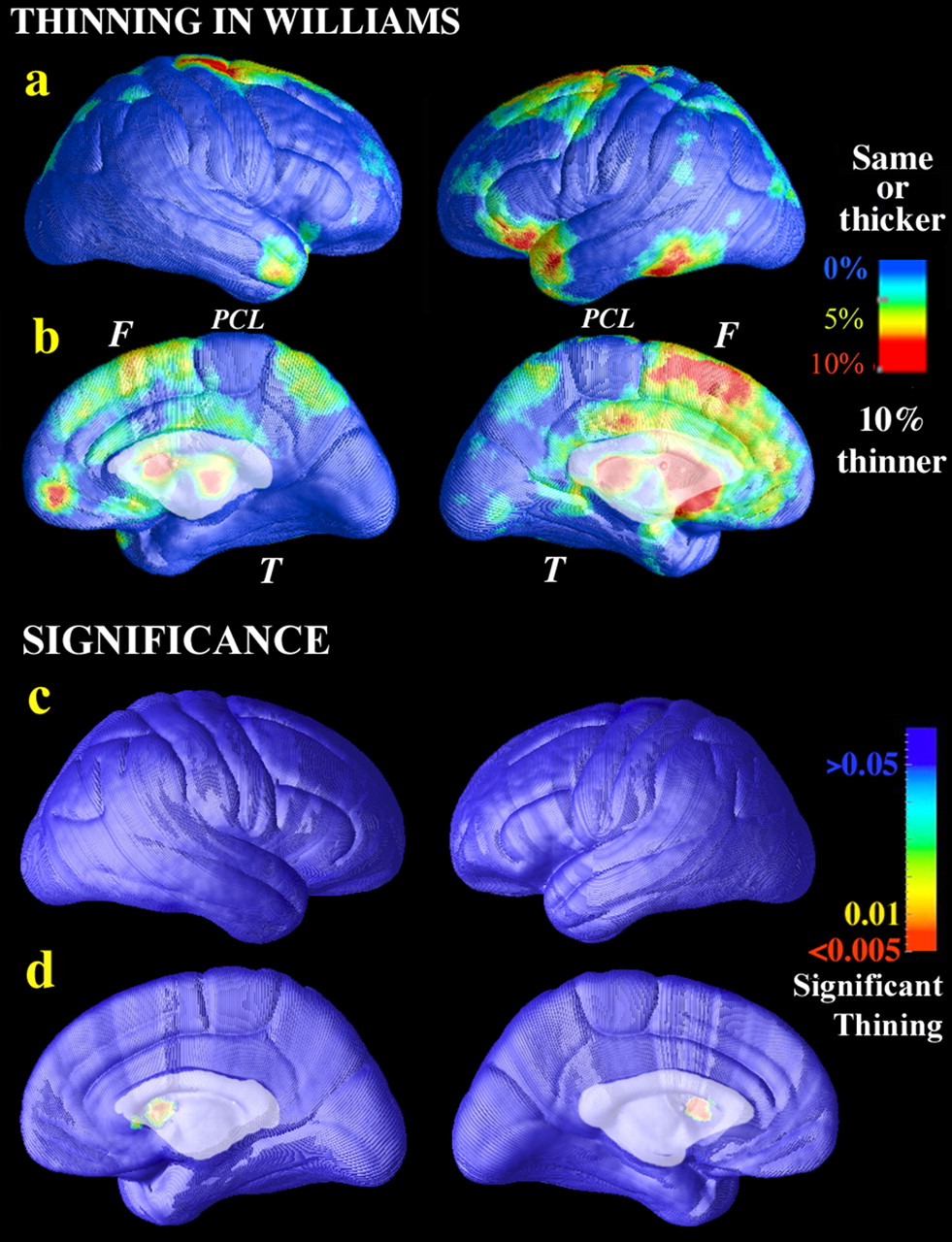
- Figure 5.
Cortical thickness maps: regional decreases in WS. In some regions of the dorsal stream, the estimated mean cortical thickness in WS was lower than the mean value in controls (a, b), but these reductions were not found to be significant (c, d) after permutation testing, which corrects for multiple comparisons. This failure of thinning to reach significance may relate to the variance in the measures of cortical thickness (Fig. 9c,d), which may be lower in histology than in MRI-based measures (in which few voxels span the cortex). Red colors in a and b denote brain regions in which mean cortical thickness was ∼10% lower than the control mean. Blue colors denote regions in which the thickness was the same or higher in WS. A recent finding of reduced superior parietal lobule volume in WS, even after adjusting for differences in brain volume (Eckert et al., 2005), is consistent with the medial superior parietal reductions seen here. F and T denote frontal and temporal cortices, respectively, and PCL denotes the paracentral lobule. Even so, postmortem architectonic measurements are not straightforwardly related to MRI findings in WS. In the visual cortex, smaller cells and increased packing have been found in the left hemisphere. This might predict thinner cortex on MRI. Occipital gray matter volumes were reduced on MRI, but the diffuse reduction in cortical thickness was not significant here after multiple-comparisons correction.
- Figure 6.
Cortical complexity is increased in WS. The mean cortical complexity and SEs are shown for controls and for WS subjects. Black and gray squares denote data points from individual subjects in the study. In WS, cortical surface complexity is increased in both brain hemispheres. This extends previous work measuring gyrification in 2D serial sections (Schmitt et al., 2002). Postmortem studies have found multiple small gyri in dorsal cortical regions (Galaburda and Bellugi, 2000), and increased fissuration is often apparent in the WS brain by visual inspection (Fig. 7). Schmitt et al. (2002) examined gyrification patterns in 17 WS subjects and 17 controls and found significantly increased cortical gyrification globally, with greater abnormalities in right parietal (p = 0.02), right occipital (p = 0.02), and left frontal (p = 0.009) regions. These regional gyrification effects (such as the increased folding shown in Fig. 7) are not so easily localized using a global measure such as fractal dimension. Hem., Hemisphere.
- Figure 7.
Gyrification differences in WS. The fissuration pattern of the precentral, central, and postcentral sulci (labeled 1, 2, and 3, respectively) is typically very simple in control subjects but more complex in WS. A typical control subject (a) and a typical WS subject (b) are shown. Note the thinner gyri in the WS subject and increased fissuration in the paracentral area. c and d show how the surface mesh models of the cortex were partitioned into lobes for a normal subject (c) and a WS subject (d). Cortical pattern matching allows corresponding regions of parameter space to index the same anatomy across subjects, allowing accurate partitioning of anatomy. The cortical registration approach used here identifies the maximal subset of sulci that occur consistently in all subjects, and these are used to align anatomy across subjects. These sulci are always present in the WS subjects as well as in controls. Even so, in individual subjects, there may be additional accessory sulci or fissures created by abnormal folding (as seen here). These sulci are not used in the anatomical normalization (because they do not have counterparts in all other brains); they are therefore situated between the major cortical sulci that are aligned.
- Figure 8.
Cortical thickness and complexity are correlated. Lateral (a) and medial (b) views of the cortex are shown. In healthy normal subjects (n = 40), higher cortical complexity is correlated with thicker cortex in right perisylvian areas, primary sensorimotor and visual cortices, and a broad band of cingulate/paracingulate cortex (p < 0.02). At each cortical location, the thickness at that location was regressed against the overall complexity value for the brain hemisphere. Regions in which there is a significant linkage between cortical thickness and hemispheric complexity are shown. No relationships were detected in the left hemisphere or in the WS subjects for either hemisphere. Our ongoing mathematical work will recast the fractal dimension as the surface integral of a fractal density measure, which is more likely to correlate pointwise with cortical thickness than global complexity measures. Such work may make it possible to compute the fractal dimension directly from the curvature tensor and metric of the cortical surface. Across species, the cerebral gray/white matter ratio obeys an allometric power law that predicts increased gray matter fissuration as brain size increases (Zhang and Sejnowski, 2000). It is unknown whether a similar power law is found within species; we recently found that mean cortical complexity was higher in women than in men (Luders et al., 2004), and women generally have a higher proportion of gray matter (relative to total brain volume) than men, consistent with a hypothetical relationship between cortical thickness and complexity.
- Figure 9.
Age effects and variation in cortical thickness. a, b, Brain regions in which significant cortical thinning with increasing age was detected (red colors). c, d, The SD in cortical thickness in the 40 controls at each point of cortex, showing the high variance in the perisylvian cortex. Maps were similar in WS (not shown in this figure). The statistical power for detecting group differences in cortical thickness is spatially variable and depends on the 3D anatomical variability of each region across subjects after data are aligned to a common space as well as the local intersubject variance in cortical thickness (c, d). High-anatomical variability typically reduces statistical power for detecting group differences (because of confounding anatomical noise). The posterior limits of the Sylvian fissures and surrounding perisylvian territory have extremely high variability (∼15-20 mm 3D rms variability in Talairach stereotaxic space) in part because of the wide variations in the termination points of the ascending and posterior branches of the Sylvian fissures and superior temporal sulci (Thompson et al., 2000, 2001a). Without efforts to overcome this variability, such as the high-dimensional anatomical normalization used in this study, there is an intrinsically lower power for finding gray matter differences in the perisylvian region, relative to other brain regions (Witelson and Kigar, 1992). This is likely why gray matter differences were not found in these regions using voxel-based morphometry (Reiss et al., 2004), because only a low-order anatomical normalization was used. A cortical pattern-matching approach is used in this study to overcome this high variability, explicitly using sulcal landmarks to align cortical regions and increase the homology of anatomical comparisons and the resulting signal-to-noise ratio. As observed in the statistical maps, there was sufficient power to detect group differences in cortical thickness in the perisylvian areas, despite their very high anatomical variability.


