

Article Figures & Data
Figures
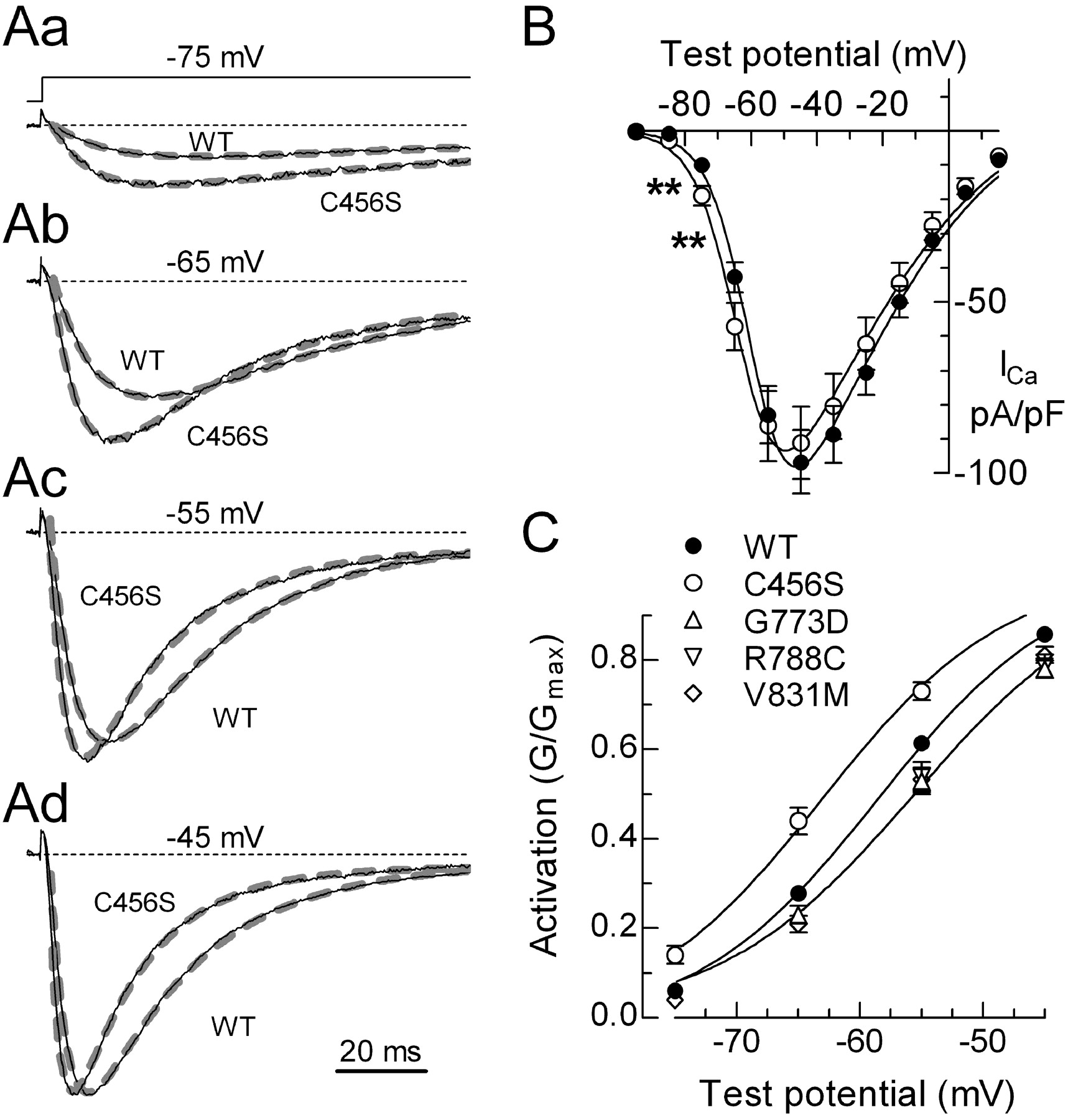
- Figure 1.
Effect of C456S on the current-voltage relationship of Cav3.2. Aa-Ad, Representative current traces recorded during depolarizing voltage steps. Schematic of the voltage protocol is shown in Aa. Holding potential was -115 mV. Zero current baseline is indicated with a dotted line. The currents were normalized to the peak current observed in that cell, which was typically observed at -45 mV. Also shown are the exponential fits (thick gray dashed lines) to the currents that were used to estimate activation and inactivation kinetics. Scale bar applies to all four sets of traces. B, Peak current-voltage relationships normalized to cell capacitance. Cells expressing C456S channels had significantly more current at negative test potentials (marked with **p < 0.01). Smooth curves represent fits to the average data using a modified form of the Goldman-Hodgkin-Katz equation (see Materials and Methods). C, To illustrate this shift in voltage dependence, activation is represented by the normalized conductance (G/Gmax). G was calculated using a derivation of Ohm's law, G = I/(VT-VR), where I is the peak current, VT is the test potential, and VR is the reversal potential. Data represent mean ± SEM, in which the number of cells used to calculate the average is reported in Table 2. Only data that were significantly different from WT is plotted. Smooth curves represent fits to the average data using a Boltzmann equation.
- Figure 2.
Effect of SNPs on Cav3.2 steady-state inactivation and persistent currents. A, Representative current traces obtained during a test pulse to -35 mV after 1 s prepulses to varying potentials. Voltage protocol is shown above the traces. The cell was held at -115 mV for 10 s between sweeps. After the last depolarizing prepulse (-55 mV), the cell was tested again with a -125 mV prepulse. Typically, 95% of the original current was recovered, thereby excluding the effect of rundown. B, Inactivation (h∞) was calculated as the fraction of current available after each prepulse (I) divided by the current recorded after the first prepulse to -125 mV (Imax). Data from each cell were fit with a Boltzmann equation, and the resulting values of V50 and k were averaged (number of cells and values reported in Table 2). Smooth curves represent the average fits. Dotted line represents the activation curve for WT channels as described in Figure 1. The activation and inactivation curves overlap at approximately -70 mV. C, The percentage of channels in the overlap region was calculated as the product of the Boltzmann functions describing each process. D, Representative current traces obtained at the end of 150 ms depolarizing pulses to -55 mV. The downward spike represents the tail current triggered by repolarization. Dotted line represents the zero current baseline. E, The residual current at 150 ms (I150) was divided by the maximal current observed in that cell (Imax), averaged, and then plotted as a function of test potential. Data represent mean ± SEM, in which the number of cells used to calculate the average is reported in Table 3. Only data that were significantly different from WT is plotted.
- Figure 3.
Effect on activation, inactivation, and deactivation kinetics. Average activation (A) and inactivation (B) kinetics for channels that significantly differed from WT. Kinetics were estimated using double-exponential fits to the currents generated during the I-V protocols (Fig. 1 A). Only data that were significantly different from WT is plotted. C, Representative tail current traces obtained after repolarization to -105 mV. The voltage protocol is shown in the inset. Thick dashed lines represent exponential fits to the tail current. D, Average deactivation kinetics for WT and variants. Data represent mean ± SEM, in which the number of cells used to calculate the average is reported in Table 3. Only data that were significantly different from WT is plotted.
- Figure 4.
Development of inactivation at subthreshold voltages. Aa-Ad, Representative current traces recorded during test pulses to -45 mV. The duration of the inactivating pulse was 0 s (Aa), 1 s (Ab), 5 s (Ac), or 10 s (Ad). Solid line represents data obtained from a cell transfected with WT channels, and the dotted line represents P648L channels. B, Average time course of inactivation at -75 mV for WT, P648L, and G784S channels. Curves represent fits to the average data.
- Figure 5.
Time course of recovery from inactivation. Aa-Ad, Representative current traces recorded during test pulses to -45 mV. Channels were inactivated by holding the membrane at -75 mV for 10 s. Recovery at -105 mV was measured after pulses of 0.01 s (Aa), 0.7 s (Ab), 3 s (Ac), or 10 s (Ad). Solid line represents data obtained from a cell transfected with WT channels, and the dotted line represents V831M channels. B, Average time course of recovery for WT and V831M channels. Curves represent fits to the average data.
- Figure 6.
Voltage dependence of activation and inactivation kinetics. A, Activation (filled symbols) and deactivation kinetics of WT (circles), C456S (triangles), and G773D currents (inverted triangles) were fit with a single equation to calculate the voltage dependence of τm (smooth curves; see Materials and Methods). B, Voltage dependence of τh (smooth curves) for WT (circles), P648L (triangles), and V831M (diamonds). Open symbols represent recovery from inactivation. The data at -95, -85, and -75 mV represent development of inactivation at near subthreshold potentials as described in Figure 4. The data at -65 and -55 mV represent the inactivation τ measured during the I-V protocol.
- Figure 7.
Simulations of RE neuron firing. Current-clamp responses to mock EPSPs (A) or IPSPs (B) using values obtained with WT and R788C channels. The EPSP pulse consisted of a +0.02 nA current injection for 100 ms. The IPSP pulse consisted of a -0.1 nA current injection for 300 ms. The minimum current injection required to trigger a Na-dependent spike during an EPSP (Ab) or after an IPSP (Bb) is shown for each channel. Latency to the first Na spike triggered by a +0.02 nA depolarization (Ac) or a -0.3 nA hyperpolarization (Bc) for each channel. The number of Na spikes triggered during a +0.02 nA depolarization of 100 ms (Ad) or after a -0.1 nA hyperpolarization of 300 ms (Bd). E282K and V831M require stronger depolarizations to trigger firing.
- Figure 8.
Spontaneous oscillations induced by G773D, G773D-R788C, and C456S in a model of TC neurons. Simulated neuron-containing G773D channels was depolarized from rest (-74 mV) by a constant current injection of either 0.065 nA (A) or 0.025 nA (B). C, The frequency of subthreshold and suprathreshold oscillations is plotted as a function of current injection. The membrane potential varied between -80 and -60 mV.
- Figure 9.
Simulations of spindle oscillations in a network model of TC and RE neurons. The biophysical properties of WT (A, B) and C456S (C, D) channels were introduced into the RE neurons. WT channels triggered spindle oscillations that were quite similar to the original model (Destexhe et al., 1996a). Traces represent the responses recorded from the soma of TC (0). The region underlined in A and C is shown in an expanded time scale in B and D, respectively.


Tables
SNPs on CAE patients CAE patients CAE SNP R788 status Allele 1 Allele 2 Patient 1 F161L (+/−) R788C (+/−) F161L R788C Father F161L (+/−) R788 (+/+) Mother F161 (+/+) R788C (+/−) Patient 2 G773D (+/−) R788C (−/−) G773D-R788C R788C Father G773D (+/−) R788C (−/−) Mother G773 (+/+) R788C (−/−) Patient 3 G773D (+/−) R788C (+/−) G773D-R788C Father G773 (+/+) R788 (+/+) Mother G773D (+/−) R788C (+/−) Patient 4 G773D (+/−) R788C (+/−) G773D-R788C Father G773D (+/−) R788C (−/−) Mother G773 (+/+) R788 (+/+) -
Zygosity is shown in parentheses, in which wild-type sequence is represented by a plus sign, and the SNP is represented by a minus sign.
-
m∞ h∞ V50 (mV) k V50 (mV) k Wild-type −54.8 ± 0.4 7.4 ± 0.1 (43) −85.5 ± 0.8 −7.2 ± 0.2 (29) F161L −53.3 ± 1.0 7.2 ± 0.2 (11) −82.3 ± 0.9* −5.9 ± 0.1 (7)** E282K −53.4 ± 0.7 7.9 ± 0.2 (15)** −83.9 ± 1.2 −6.3 ± 0.1 (7)* C456S −59.9 ± 0.9** 7.4 ± 0.1 (26) −85.1 ± 1.0 −6.8 ± 0.1 (16) G499S −54.2 ± 0.6 7.4 ± 0.2 (13) −85.5 ± 1.6 −7.2 ± 0.4 (8) P648L −53.9 ± 0.5 7.5 ± 0.2 (19) −81.7 ± 1.7* −6.7 ± 0.3 (8) R744Q −53.9 ± 0.6 7.4 ± 0.1 (15) −84.2 ± 2.0 −6.6 ± 0.3 (7) A748V −56.2 ± 1.1 7.1 ± 0.2 (9) −85.5 ± 1.4 −6.6 ± 0.2 (5) G773D −51.8 ± 1.0** 8.0 ± 0.2 (15)** −82.2 ± 1.1* −8.0 ± 0.4 (8)* G784S −54.0 ± 0.6 7.3 ± 0.2 (21) −85.4 ± 1.6 −6.6 ± 0.3 (10) R788C −52.5 ± 0.9* 7.9 ± 0.2 (13)* −83.2 ± 1.1 −8.5 ± 0.2 (7)** G773D-R788C −53.0 ± 0.9 7.4 ± 0.1 (7) −84.8 ± 1.5 −8.5 ± 0.5 (7)** V831M −52.2 ± 0.8** 7.5 ± 0.1 (14) −86.5 ± 1.3 −6.7 ± 0.2 (8) G848S −54.6 ± 0.8 7.1 ± 0.1 (16) −83.3 ± 2.1 −6.6 ± 0.3 (7) D1463N −52.8 ± 0.8 7.4 ± 0.2 (8) −85.8 ± 0.7 −6.3 ± 0.4 (4) -
The values of V50 and k were calculated for each cell and then averaged. Data shown are mean ± SEM from the number of cells shown in parentheses. Statistically significant differences (determined with Student's t test) are marked with a single asterisk if p < 0.05 and with a double asterisk if p < 0.01.
-
Activation τ Deactivation τ Recovery Inactivation τ Persistent current −55 mV (ms) −15 mV (ms) −105 (ms) −105 mV (ms) −75 mV (ms) −55 mV (ms) −15 mV (ms) −65 mV (% max) Wild-type 6.2 ± 0.2 2.1 ± 0.1 (36) 2.8 ± 0.1 (16) 2648 ± 154 (33) 474 ± 68(12) 23.5 ± 0.9 15.1 ± 0.4 (36) 8.5 ± 0.3 (43) F161L 6.8 ± 0.3 2.1 ± 0.1 (8) 3.2 ± 0.2 (4) 2092 ± 480 (3) 212 ± 48 (3) 26.4 ± 2.1 12.9 ± 0.51 (9)* 7.9 ± 0.6 (11) E282K 6.3 ± 0.3 2.4 ± 0.2 (16) 3.4 ± 0.6 (3) 24.4 ± 1.3 15.5 ± 0.5 (16) 7.8 ± 0.6 (16) C456S 5.1 ± 0.6* 1.6 ± 0.1 (17)** 2.7 ± 0.3 (6) 2838 ± 302 (4) 506 ± 101 (5) 20.2 ± 1.5 14.8 ± 0.6 (17) 6.7 ± 0.7 (17)** G499S 6.6 ± 0.6 2.1 ± 0.1 (12) 3.1 ± 0.2 (5) 2612 ± 820 (3) 374 ± 114 (3) 24.7 ± 1.5 16.2 ± 0.7 (12) 10.0 ± 0.6 (13)* P648L 6.6 ± 0.4 2.2 ± 0.1 (19) 3.0 ± 0.2 (5) 2052 ± 289 (7) 1686 ± 749 (5)* 27.7 ± 1.1** 16.1 ± 0.4 (19) 9.7 ± 0.3 (21)* R744Q 6.8 ± 0.5 2.2 ± 0.2 (15) 3.2 ± 0.3 (6) 24.7 ± 1.3 15.3 ± 0.7 (15) 9.4 ± 0.6 (16) A748V 5.4 ± 0.3* 1.9 ± 0.1 (9) 3.0 ± 0.3 (4) 21.6 ± 1.0 14.6 ± 0.5 (9) 8.7 ± 0.3 (9) G773D 8.4 ± 0.6** 2.9 ± 0.2 (11)** 3.6 ± 0.2 (6)** 1875 ± 438 (5) 799 ± 267 (4) 31.0 ± 1.8** 19.2 ± 0.6 (11)** 10.9 ± 0.7 (15)** G784S 7.1 ± 0.4* 2.1 ± 0.1 (21) 3.2 ± 0.2 (6) 2611 ± 217 (9) 248 ± 43 (7)* 24.9 ± 1.2 15.1 ± 0.5 (21) 8.6 ± 0.4 (21) R788C 7.2 ± 0.9 2.6 ± 0.2 (8)* 3.3 ± 0.2 (6)* 2038 ± 126 (6) 424 ± 15 (3) 32.6 ± 2.1** 17.1 ± 0.7 (8)* 11.3 ± 0.4 (9)** G773D-R788C 6.4 ± 0.6 2.3 ± 0.1 (7) 3.6 ± 0.1 (2)* 25.6 ± 3.1 15.3 ± 0.4 (7) 9.1 ± 0.3 (7) V831M 7.2 ± 0.3** 2.2 ± 0.1 (13) 3.4 ± 0.1 (7)* 1845 ± 234 (7)* 595 ± 190 (4) 31.6 ± 3.0** 16.9 ± 0.6 (13)* 9.4 ± 0.6 (15) G848S 6.7 ± 0.3 2.2 ± 0.1 (14) 3.5 ± 0.1 (6)** 25.1 ± 1.9 15.7 ± 0.8 (14) 9.1 ± 0.7 (16) D1463N 6.5 ± 0.5 1.8 ± 0.1 (8)* 3.3 ± 0.1 (4) 24.6 ± 1.8 14.3 ± 0.8 (8) 7.8 ± 0.6 (8) -
Data shown are mean ± SEM from the number of cells shown in parentheses. Data at −55 and −15 mV are from the same cells. Statistically significant differences are marked with a single asterisk if p < 0.05 and with a double asterisk if p < 0.01.
-


