

Abstract
Cortical networks generate temporally correlated brain activity. To clarify the functional significance of this correlated activity, we asked whether and how its structure depends on stimulus and arousal state. Using independent components analysis of macaque functional magnetic resonance imaging data, we identified a large number of brain networks that were strikingly reproducible across different visual stimulus contexts. Fewer networks were reproducible across alert and anesthetized brain states. Network complexity ranged from bilateral single-node networks to networks comprising multiple discrete nodes distributed over 3 cm of cortex; one network identified in our survey included parts of the temporal parietal occipital junction, dorsal premotor cortex, insula, and posterior cingulate cortex bilaterally. Our results reveal the wealth of spatially structured correlated networks throughout the brain in both alert and anesthetized monkeys, and show that anesthesia significantly alters the spatial structure of these networks.
Introduction
The brain is a highly interconnected dynamic system. As a consequence, activity in different parts of the brain can be temporally correlated, and this correlated activity can be used to partition the brain into discrete networks (McKeown et al., 1998; Raichle and Mintun, 2006). Some of these temporal correlations are stimulus-driven, whereas others stem from “spontaneous” activity. Correlated fluctuations in spontaneous activity have been observed at multiple spatial scales and using a variety of techniques including single-unit and local field potential recordings (Engel and Singer, 2001; Leopold et al., 2003; Fiser et al., 2004), optical imaging (Arieli et al., 1996), EEG and magnetoencephalography (Lachaux et al., 1999), and functional magnetic resonance imaging (fMRI) (Biswal et al., 1995; Xiong et al., 1999). The origin and function of spontaneous fluctuations are not well understood (Raichle and Mintun, 2006). Spontaneous fluctuations could reflect neural noise within anatomically connected areas (Shadlen and Movshon, 1999); alternatively, they could result from active mechanisms and play an important role in perception and awareness (Singer and Gray, 1995). fMRI, which records whole brain activity at high spatial resolution, provides a powerful tool to observe correlated activity, both stimulus-driven and spontaneous, across the brain at a time scale slower than 0.1 Hz, and to test its functional significance. Only one previous study has explored functional connectivity in monkeys using fMRI data; this study revealed that large-scale correlated brain networks exist in anesthetized macaques (Vincent et al., 2007).
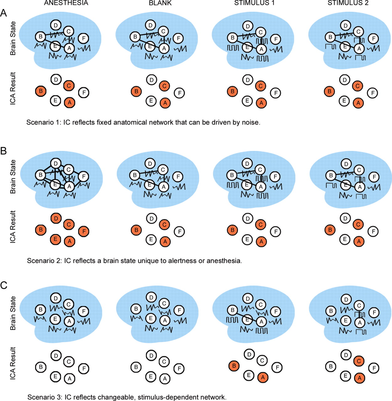
To understand the functional significance of correlated brain activity, it is necessary to know whether and how its structure depends on stimulus and arousal state. Here, we applied spatial independent components analysis (ICA) to fMRI data obtained from both alert and anesthetized macaques and across different visual stimulus contexts. ICA provides a mathematical technique to identify functionally connected networks (McKeown et al., 1998) (see Materials and Methods). Our goal was to partition the brain in each stimulus and arousal state, and then compare the structure of identified networks across states. We reasoned that if the structure of a network remains constant regardless of stimulus or arousal state, then the network likely reflects hard-wired anatomical connections that are spontaneously active (Fig. 1A). If the structure of a network depends on arousal state, but remains constant regardless of stimulus state (including the case of no stimulus at all), then the network likely reflects a brain state unique to alertness or anesthesia (Fig. 1B). Finally, if the structure of a network is modulated by specific stimuli, then the network likely reflects a changeable, stimulus-dependent brain state (Fig. 1C). Therefore, characterizing the dependence of correlated networks on stimulus and arousal state should contribute to understanding the origin and functional significance of these networks. Furthermore, characterizing these networks in macaques makes it possible to link insights into functional connectivity derived from fMRI to a large body of work on structural and functional connectivity derived from single-unit electrophysiology and classic anatomical tracing in macaques (Felleman and Van Essen, 1991; Munk et al., 1996; Leopold et al., 2003).

Three scenarios for the dependence of ICs on stimulus and arousal state. A, If the structure of a network remains constant regardless of stimulus or arousal state (i.e., columns 1–4 yield the same ICA result), then the network likely reflects fixed anatomical connections that can be driven by spontaneous activity. B, If the structure of a network remains constant regardless of the stimulus state (i.e., columns 2–4 yield the same ICA result), but does depend on the arousal state (e.g., showing greater or less connectivity during anesthesia, column 1), then the network likely reflects a brain state unique to alertness or anesthesia. C, If the structure of a network depends on the presence of specific stimuli, then the network likely reflects a changeable, stimulus-dependent brain state.
Materials and Methods
All animal procedures complied with the NIH Guide for Care and Use of Laboratory Animals, regulations for the welfare of experimental animals issued by the Federal Government of Germany, and stipulations of Bremen authorities.
Subjects
Five rhesus macaque monkeys (weight: 3–6 kg, age: 3–6 years) were used for this study.
Monkey surgery
The implantation of the MR-compatible headpost (Ultem, General Electric Plastics) followed standard anesthetic, aseptic, and postoperative treatment protocols which have been described in detail previously (Wegener et al., 2004). MR-compatible ceramic screws (Thomas Recording) and acrylic cement (Grip Cement, Caulk; Dentsply International) were used to secure the headpost to the skull.
Visual task
For the alert monkey fMRI experiments, monkeys were required to fixate inside the scanner on a small fixation spot (0.36° diameter) in exchange for a juice reward. The fixation window size was up to 6°, and fixation time was 3 s. Eye movements were monitored inside the scanner with a pupil/corneal reflection tracking system (RK-726PCI, Iscan).
Sinerem injections
Figures 2 and 3, and supplemental Figures S3 and S5 (available at www.jneurosci.org as supplemental material) are based on blood oxygen level-dependent (BOLD) signals. Data for the remaining figures were obtained with a contrast agent, ferumoxtran-10 (Sinerem, Guerbet; concentration: 21 mg Fe/ml in saline; dosage: 8 mg Fe/kg) that was injected into the femoral vein before each scan session. Sinerem is the same compound as MION, produced under a different name (Nelissen et al., 2005). Sinerem/MION increases signal-to-noise and gives finer spatial localization than BOLD (Vanduffel et al., 2001; Leite et al., 2002; Zhao et al., 2006). Sinerem results in a signal reduction at activated voxels; for all functional data we inverted the signal to facilitate comparison with BOLD data.
Anesthesia
For anesthetized monkey experiments (see Fig. 7), two monkeys were given an initial dose of atropine (0.05 mg/kg) and ketamine/medetomidine (8 mg/kg, 0.04 mg/kg). A maintenance dose of 4 mg/kg ketamine was given after 2 h of scanning. The eyes were covered with antibiotic ointment and closed, and this was also monitored through the ISCAN system. Respiration rate was monitored during scanning.
Visual stimuli
Visual stimuli were projected from an LCD projector (1280 × 1024 pixels, 60 Hz refresh rate), onto a screen positioned 49 cm in front of the monkey's eyes. The display spanned 32 cm laterally and 24 cm vertically. Visual stimuli were generated on a Dell Latitude laptop in MATLAB, using the Psychophysics Toolbox extensions (Brainard, 1997; Pelli, 1997). Stimuli consisted of: clips from “James Bond, Tomorrow Never Dies” (see Figs. 2, 3; supplemental Fig. S5, available at www.jneurosci.org as supplemental material), a set of 6 visual localizer stimuli (see Figs. 4⇓–6, 8, 9; supplemental Figs. S7–S9, S12A), and a blank screen with a fixation spot (see Figs. 6, 8C; supplemental Fig. S12B, available at www.jneurosci.org as supplemental material). A schematic of each of the visual stimuli, including stimulus timing, is shown in supplemental Figure S1, available at www.jneurosci.org as supplemental material. For the blank stimulus in Figure 6, the stimulus consisted of a blank gray screen with a fixation spot in the center. For the blank stimulus in supplemental Figure S11, available at www.jneurosci.org as supplemental material, the projector was turned off and the room was completely dark.
Magnetic resonance imaging
Scanning was performed in a Siemens 3 T Allegra scanner. A custom send/receive surface coil was used to acquire functional scans. Data in Figures 2 and 3, and supplemental Figs. S5 and S11 (available at www.jneurosci.org as supplemental material) were obtained using echoplanar imaging (EPI), 64 × 64 matrix, repetition time (TR) = 3, 42 slices, 1.25 × 1.25 × 1.75 mm voxels. Data for remaining figures: multiecho EPI sequence, TR = 4 s; 64 × 64 matrix; 28 slices, 1.25 × 1.25 × 1.25 mm voxels (see Figs. 4⇓–6, 8, 9; supplemental Figs. S7, S9, S12, available at www.neurosci.org as supplemental material) or TR = 4 s; 64 × 64 matrix; 42 slices, 1.5 × 1.5 × 1.5 mm voxels (see Fig. 7). The multiecho sequence allowed subsequent EPI undistortion based on the field map (Zeng and Constable, 2002; Cusack et al., 2003), facilitating registration of functional data to high resolution anatomical data. Each scan session was ∼3 h long. In total, we obtained 6 movie sessions, 36 localizer sessions, 6 blank sessions, and 2 anesthesia sessions.
Data analysis
Preprocessing
Data were motion corrected using the “AFNI” motion correction algorithm (Cox and Hyde, 1997) and spatially smoothed using a 3D Gaussian kernel with full width at half maximum of 2 mm.
General linear model analysis.
General linear model (GLM)-based analysis of fMRI data used FSFAST (http://surfer.nmr.mgh.harvard.edu), following procedures detailed in the study by Tsao et al. (2003).
Identifying functionally connected networks with independent components analysis.
The two approaches that have been developed to extract functionally connected networks from fMRI data, seed-based correlation analysis and ICA, both have advantages and disadvantages.
Seed-based correlation analysis (Biswal et al., 1995; Fox et al., 2005, 2006a; Vincent et al., 2006, 2007) requires specification of a seed location (based on either a priori anatomical knowledge or results of functional imaging experiments in which regions of interest have been identified), whose time course is then correlated to time courses of voxels from the rest of the brain. An advantage of seed-based correlation analysis is that results can be simply interpreted in terms of correlation coefficients. A disadvantage is that seeds need to be specified in advance, requiring one to possess prior knowledge about the location of functional networks of interest, and limiting the number of networks that can be identified. A simulation study found that in the presence of structured noise [common in fMRI data, due to physiological artifacts, ghosting, and head motion (Krüger and Glover, 2001)], networks detected with seed-based correlation analysis depend strongly on the precise location of chosen seeds (Ma et al., 2007).
An alternative approach for identifying functionally connected networks is ICA (McKeown et al., 1998; Calhoun et al., 2001, 2004; Beckmann et al., 2005; Beckmann and Smith, 2005; Calhoun and Adali, 2006). ICA comprehensively partitions the brain into multiple statistically independent networks without requiring any prior knowledge about the functional or anatomical characteristics of the cortical areas involved. ICA, a method for “blind source separation,” separates an observed “mixture” into statistically independent “sources” (Bell and Sejnowski, 1995). In the case of fMRI, the term mixture refers to the collection of voxel activation values recorded at a series of time points, whereas the term source refers roughly to a subset of these voxels that coactivates temporally (McKeown et al., 1998). Put more precisely, sources are sets of voxel weights that represent statistically independent spatial patterns, or equivalently, spatial patterns with maximal information content and minimal mutual information. A simulation study comparing performance of ICA to that of seed-based correlation analysis concluded that ICA is superior when structured noise is strong (Ma et al., 2007), due to its ability to factor out structured noise as a separate independent component (IC). Another study comparing brain networks activated by a finger-tapping task identified by seed-based correlation analysis and by ICA found that seed-based correlation analysis yielded a single motor network, whereas ICA further partitioned this network into two distinct networks with different power spectra (Beckmann et al., 2005). Thus ICA is capable of distinguishing networks with partially correlated time courses that tend to be grouped together by seed-based correlation analysis.
A large number of studies have identified correlated brain networks from fMRI data in humans, using both seed-based correlation analysis (Biswal et al., 1995; Xiong et al., 1999; Fox et al., 2005, 2006a,b; Fransson, 2005; Raichle and Mintun, 2006; Vincent et al., 2006, 2007; Greicius et al., 2007) and ICA (Bartels and Zeki, 2004, 2005a,b; van de Ven et al., 2004; Beckmann et al., 2005; Beckmann and Smith, 2005).
In the present study, ICA was performed using FMRIB Software Library (FSL) MELODIC (multivariate exploratory linear optimized decomposition into independent components). This software performs spatial independent components analysis on 4D volumes. Details are described in the study by Beckmann and Smith (2004). Instead of dissecting the input data into the maximum allowed number of components, MELODIC by default estimates the number of independent components that should be computed (the model order) using PCA and Bayesian inference. Although the number of components can be specified explicitly in MELODIC, specifying too low a number of components sacrifices the ability of ICA to separate noisy ICs from data of interest. However, specifying a number of components that is too high can result in artificial splitting of coherent networks into separate ICs. As such, MELODIC's built-in model order selection tool was used for all analyses. In addition, MELODIC default parameters were used for high pass filtering, brain extraction, variance normalization, and IC map thresholding.
Picking real ICs from artifacts.
For each stimulus, fMRI data were acquired in a minimum of 2 independent scan sessions, each with ∼10 runs. The initial ICA on these data sets yielded between 300 and 1000 ICs per session. Many of these constituted artifacts. We used a 3 step semiautomated procedure to extract a set of unique, real ICs from these potential targets. (1) Selection of bilateral ICs (automated): If an IC is bilateral, this greatly increases the chance that it represents a real network; there is no reason why measurement noise should appear bilaterally, but strong connections between the two hemispheres are known to generate functional interactions between them (Fox et al., 2006a). Therefore, we assigned a bilaterality score to each IC by computing the level of correlation between the spatial pattern of activity in the left and right hemispheres. Only the 200 ICs from each session with the highest bilaterality scores were considered for further analysis. The bilaterality score was defined by the following:
 where N is the number of slices, lrdiff is the difference between the left half of a slice and the right half flipped horizontally, and lravg is the product of the two. When an IC is perfectly symmetric, lrdiff = 0, diffi is at a minimum, and the bilaterality score is maximum. Obviously, lateralized ICs can also constitute useful candidates; e.g., the language network is known to be strongly lateralized (Liégeois et al., 2002). Our set of culled networks likely represents only a subset of the full set of statistically independent networks. (2) Selection of nonartifactual ICs (manual): For each scan session, the 200 remaining ICs were individually screened, and manually assigned to one of three categories: “artifact,” “unclear,” or “not an artifact.” Supplemental Figure S2A, available at www.jneurosci.org as supplemental material, displays various cases of artifacts; artifacts included ventricles, zebra stripe patterns, and random speckle throughout the brain. In particular, bilateral artifacts due to head motion generate a distinctive activation pattern around the rim of the brain (supplemental Figure S2A, top left, available at www.jneurosci.org as supplemental material). In addition to artifacts, ICA also identified multiple bilateral subcortical ICs in the cerebellum, brainstem, and basal ganglia (supplemental Figure S2B, available at www.jneurosci.org as supplemental material). These were also excluded from further analysis. The present study focuses on clearly nonartifactual, cortical ICs. We used a conservative criterion, excluding both ICs that were clearly artifactual (e.g., the ones following the rim of the brain, ventricles) as well as “unclear” ICs that may have corresponded to real functionally connected networks (supplemental Fig. S2A, available at www.jneurosci.org as supplemental material, second row, rightmost two ICs). A future improvement would be to develop image processing algorithms that can discard artifacts automatically. (3) Selection of unique ICs across scan sessions (automated): Because ICA was performed independently on data from multiple independent scan sessions, a particular functional interaction could be represented by multiple (spatially correlated) ICs when pooling data across scan sessions. Therefore, it was necessary to eliminate redundancies in generating a final set of real ICs. To select representative unique ICs, we first ranked all the ICs remaining after steps 1 and 2 by computing an “IC quality score” as follows. To obtain a measure of reproducibility, for each session, each IC was correlated with all of the ICs from each of the other sessions, and the mean of the maximum intersession correlations was taken as the reproducibility score for that IC. The reproducibility score and the bilaterality scores were then multiplied to yield an IC quality score. The multiplication operation was chosen to ensure that ICs scoring poorly in either reproducibility or bilaterality would be penalized in the overall quality score. Unique ICs were selected by proceeding from highest to lowest through the list of ICs ranked by their quality scores, eliminating lower-ranking ICs if the spatial correlation to a higher-ranking IC was >0.22 (see below for justification).
Comparing ICs across stimulus conditions.
To identify matching components across different stimulus conditions (see Figs. 5, 8, 9; supplemental Fig. S9, available at www.jneurosci.org as supplemental material), for each IC in a given stimulus condition, we computed the spatial correlation to ICs in each of the five other stimulus conditions. An IC with r > 0.1 was classified as a matching IC (see below for justification).
Choice of correlation thresholds.
The r = 0.22 threshold represents an upper bound on similarity between unique ICs, whereas the r = 0.1 threshold represents a lower bound on the similarity of reproducible ICs. The r = 0.22 threshold was derived using a bootstrap procedure as follows. For every possible IC pair among the ICs remaining after the 3-step culling procedure, a spatial correlation coefficient was computed. From this distribution, correlation coefficients were shuffled and sampled 1000 times, and the lowest correlation value in the top 5% of the subpopulation (statistic of interest) was computed on each sample. From the resulting distribution for this statistic of interest (which can be reasonably approximated as Gaussian), we estimated a p = 0.05 significance level for IC similarity. The correlation value arrived at by applying this bootstrapping procedure was 0.22, and as such, the lower-scoring IC in any pair of ICs with spatial correlation >0.22 was removed to create the set of “unique” ICs.
We used a lower threshold (r = 0.1) to set a lower bound on the similarity of reproducible ICs. The difference between the two spatial correlation thresholds used reflects differences in their applications. The r = 0.22 uniqueness threshold (calculated using the bootstrapping procedure just described) is strict to ensure that no two similar ICs are reported as different networks, whereas the r = 0.1 reproducibility threshold (obtained using visual inspection), is slightly relaxed to allow for small variations in spatial structure of ICs across stimuli. To ensure the validity of the results shown in Figure 5 regarding IC reproducibility, supplemental Figure S8, available at www.jneurosci.org as supplemental material, has been included, in which the stricter r = 0.22 threshold was used.
Rendering data onto flattened patches.
We used FreeSurfer (http://surfer.nmr.mgh.harvard.edu) to reconstruct cortical surfaces from high resolution anatomical data and to visualize functional data on flattened patches and inflated brain surfaces, following procedures described by Tsao et al. (2003). Functional data were manually coregistered with high resolution anatomical data in an iterative procedure allowing rotation, translation, and single-axis scaling. Surface data were smoothed with a Gaussian smoothing kernel (2 mm full-width at half-maximum).
Results
In this study, we compare the spatial structure of ICs obtained across four different stimulus/arousal conditions: (1) viewing a rich movie stimulus, (2) viewing a set of six visual localizer stimuli tailored to activate specific visual modalities, (3) viewing a blank screen, and (4) anesthesia.
Identifying ICs using a rich movie stimulus
In our first experiment, we scanned two monkeys (monkeys L, H) while they viewed clips of the James Bond film “Tomorrow Never Dies,” interleaved with three blank periods. Supplemental Figure S1, available at www.jneurosci.org as supplemental material, shows a schematic of the stimulus sequence. We chose to use a visually rich movie stimulus containing multiple shapes, animate forms, motions, and colors to activate as large a number of visual networks as possible (Hasson et al., 2004; Bartels and Zeki, 2005a)
Each monkey was scanned in three separate scan sessions. ICs for each scan session were computed using MELODIC software (Beckmann and Smith, 2004) (see Materials and Methods for details). Given a 4D volume (three spatial dimensions × time), spatial ICA can yield as many ICs as there are data points in the time dimension; for a data set with 136 time points * 10 repetitions, there are potentially 1360 different ICs In practice, MELODIC was run using a built-in tool to estimate the number of ICs into which a 4D volume should be separated (see Materials and Methods for details), yielding sets of 300–1000 ICs.
Many of these ICs consist of artifacts; indeed, ICA can be specifically used to remove data artifacts (Thomas et al., 2002; Iriarte et al., 2003; Beckmann et al., 2005). To identify a set of real ICs, we performed a stringent 3-step selection procedure, retaining only bilateral, nonartifactual ICs that were reproducible across independent scan sessions (see Materials and Methods for details). This conservative procedure likely discarded some ICs that corresponded to real networks, e.g., strongly lateralized ICs The focus of the current study was not to comprehensively identify all coherent networks in the macaque brain, but to compare ICs across stimulus and arousal states; importantly, we applied the same culling procedure for all experiments.
The 20 networks remaining after application of the three-step culling procedure to fMRI data collected for one monkey (monkey L) using the James Bond movie stimulus are shown in Figure 2A (supplemental Figure S3, available at www.jneurosci.org as supplemental material, shows the same ICs in slice format). Networks covered visual, auditory, somatosensory, motor, prefrontal, and parietal regions. One of the identified networks corresponded to the frontal eye field–lateral intraparietal area (FEF–LIP) network (Fig. 2A, network #17) known to be important for planning eye movements (Schall, 1991) and controlling attention (Corbetta, 1998). This network was previously identified on the basis of correlated spontaneous activity in anesthetized macaques using seed-based correlation analysis (Vincent et al., 2007). Together, the 20 ICs covered a significant fraction of the entire brain (Fig. 2B).

ICs from one animal (monkey L). The stimulus consisted of movie clips from “James Bond, Tomorrow Never Dies” (see supplemental Fig. S1A, available at www.jneurosci.org as supplemental material, for a summary of the stimulus sequence). A, All 20 ICs determined to represent functional networks based on an IC quality score combining reproducibility across days and bilaterality (see Materials and Methods for details). The ICs are rendered on inflated cortical surfaces and are ordered according to their IC score. B, The ICs in A are overlaid on a single surface to show the overall extent of brain coverage. The color scale bar shown here applies to all figures in this study.
Reproducibility of ICs across days
Most ICs were highly reproducible across independent scan sessions. Figure 3A shows the matrix of spatial correlations between the 20 ICs shown in Figure 2 and their 20 best intersession correlators (i.e., the bilateral, nonartifactual IC from a different scan session using the same stimulus which had the highest correlation to the given IC). The high values along the diagonal indicate that most of the ICs were reproducible across scan sessions. The lack of high intersession correlation values off the diagonal indicates high specificity of ICs. Two example ICs and their best intersession correlators are shown in Figure 3, B and C (the same data are shown in inflated format in supplemental Figure S4, available at www.jneurosci.org as supplemental material). Some variability in IC spatial structure between days can be observed, e.g., in Figure 3C, LIP appears stronger in the left panel.

Spatial reproducibility of ICs. A, Matrix of spatial correlation values between the 20 ICs shown in Figure 2 and the set of 20 “best intersession correlators.” For each IC, the best intersession correlator was defined as the IC obtained from an independent scan session using the same stimulus showing the highest spatial correlation. B, C, Coronal slices (from posterior to anterior) showing two ICs (left) and their best intersession correlators (right). The two ICs are indicated by the black squares in A. Num, Number.
Clustering of ICs
Evidence exists for two anticorrelated clusters of networks in the human brain, which can be observed in the resting state from the structure of spontaneous correlations (Fox et al., 2005; Golland et al., 2007). In one animal we observed that ICs were grouped in two clusters, with IC time courses correlated within a cluster, and anti-correlated across clusters (supplemental Figures S5, S6, available at www.jneurosci.org as supplemental material). Results in four other animals were less clear.
Stimulus dependence of ICs
The ICs in Figure 2 were obtained from data in which the monkey viewed a movie stimulus containing multiple types of visual information (color, motion, depth, faces, objects, bodies, etc.). Because different parts of visual cortex are known to be specialized for representing different types of visual information (Zeki, 1978), one might expect the spatial structure of ICs in visual cortex to depend strongly on the particular visual stimulus being viewed. To determine the stimulus dependence of ICs, we ran three monkeys (monkeys E, M, and B) on six different visual stimuli: a retinotopic localizer stimulus, a disparity stimulus, a random-dot motion stimulus, a face localizer stimulus, a colored shapes stimulus, and a 3D paperclip stimulus (supplemental Fig. S1, available at www.jneurosci.org as supplemental material).
Before comparing ICs across stimuli, we first verified that ICA was able to extract stimulus-driven networks known from traditional GLM analysis (Friston et al., 1995) to be activated by each of these six stimuli. Figure 4A shows results of a standard GLM analysis of retinotopy data: comparison of responses to a vertical vs horizontal wedge revealed the well known retinotopy of macaque visual cortex, with different areas separated, alternately, by the vertical and horizontal meridians (Brewer et al., 2002; Fize et al., 2003). Figure 4B shows two ICs obtained from the same data set (retinotopic localizer stimulus). IC 1 corresponds to representations of the vertical meridian, IC 2 to representations of the horizontal meridian. As a second example of the efficacy of ICA for revealing stimulus-driven networks, Figure 4C shows results from a standard GLM analysis of data collected while the monkey viewed disparity-defined shapes that alternated with a zero disparity pattern. Activation was observed in areas V3, V3A, and caudal intraparietal sulcus (CIPS), consistent with previous fMRI results (Tsao et al., 2003). ICA of the same data set revealed an IC that matched the GLM-based map of disparity-driven areas (Fig. 4D).

ICA reveals stimulus-driven networks (monkey B). A, Retinotopic map obtained by comparing the response to a vertical wedge vs a horizontal wedge. The solid lines indicate representations of the horizontal meridian and dotted lines representations of the vertical meridian. B, Top, ICA of the same data set as in A revealed the two ICs shown here (as well as many others). IC 1 corresponds to the representation of the vertical meridian, IC 2 to the representation of the horizontal meridian (the numbering of the ICs here is arbitrary). C, Map of areas activated by disparity-defined shapes compared with a zero-disparity plane (see supplemental Fig. S2C, available at www.jneurosci.org as supplemental material, for stimulus details). D, IC obtained from ICA of the same data set as in C. IC 1 corresponds to the map of 3D-selective areas revealed by the GLM comparison in C.
Having verified the efficacy (Figs. 2, 4) and robustness (Fig. 3) of ICA, we proceeded to compare the spatial structure of ICs across stimulus conditions. For each of the six stimulus sets, we obtained fMRI data in two separate scan sessions. Then, we followed the same procedure as described above for Figure 2 to select a set of bilateral, nonartifactual ICs for each stimulus set in each monkey. This procedure produced a variable number (between 8 and 29) of ICs per stimulus set, precluding a one-to-one identification of ICs across stimulus sets, but we can still ask: for each IC from a given stimulus condition, what is the highest value of spatial correlation obtained across ICs from a different stimulus condition? Supplemental Figure S7, available at www.jneurosci.org as supplemental material, shows the spatial correlation between ICs under different visual stimulus conditions for three monkeys (monkeys E, M, and B). A total of 36 correlation matrices are shown, one for each stimulus pair. Many ICs were reproducible across different stimuli. But the fact that same-stimulus correlation matrices had the more distinct diagonals (monkey E, mean diagonal correlation value = 0.26; monkey M, mean = 0.25, monkey B, mean = 0.24) than different-stimulus correlation matrices (monkey E, mean = 0.19; monkey M, mean = 0.21, monkey B, mean = 0.18) implies that the spatial pattern of ICs was most reproducible for repetitions of the same stimulus (monkey E, p < 0.001; monkey M, p = 0.02, monkey B, p = 0.001, Mann–Whitney U test)
Figure 5 quantifies the reproducibility of ICs across different stimulus conditions. For each of the six stimulus sets, almost all of the selected (bilateral and nonartifactual) ICs were reproducible. The criterion for reproducibility was r > 0.1; note that this criterion allows some variation in the precise spatial structure of the IC (Fig. 3). The results of the same analysis computed with a higher threshold, r > 0.22, are shown in supplemental Figure S8, available at www.jneurosci.org as supplemental material. Furthermore, almost all of the ICs were reproducible with both the same and at least one different stimulus (Fig. 5A). Figure 5B shows, for ICs obtained with each stimulus condition, the mean fraction of ICs from the five other stimulus conditions that were spatially correlated (r > 0.1); for example, if, for every IC obtained with a given stimulus, each of the five other stimulus sets produced at least one correlated IC, then the mean fraction of correlated ICs would be 1. For all six stimuli, this fraction was >0.5. Differences between ICs across different stimulus conditions were likely due to differences in stimulus content (e.g., faces, motion, depth), although we cannot rule out that differences in stimulus size also played a role. For those ICs reproducible with both the same and different stimuli, use of the same stimulus did not lead to a higher mean spatial correlation value than use of different stimuli (Fig. 5C). Overall, the strong reproducibility of different ICs, independent of the particular stimulus, suggests that by and large ICs represent hard-wired anatomical networks that are either spontaneously active or consistently recruited for visual computations regardless of stimulus content However, it was not the case that all networks known to be anatomically connected appeared as ICs regardless of stimulus content. For example, face-selective patches in the temporal lobe are known to be strongly anatomically connected (Moeller et al., 2008), but they did not appear as an IC in response to the blank stimulus. The factors governing which anatomically connected networks are observable by ICA and which are not are unclear at this point and need to be investigated.

Classification of ICs based on reproducibility under different visual stimulus states (analysis based on the same data set as in supplemental Figure S7, available at www.jneurosci.org as supplemental material). A, Bar graph showing the total number of ICs (dark blue bars), the number of ICs that were reproducible with the same stimulus and at least one different stimulus (cyan bars), and the number of ICs reproducible only with the same stimulus (yellow bars on top of cyan bars). The criterion for reproducibility was r > 0.1. B, Bar graph showing, for ICs obtained with each stimulus condition, the mean fraction of ICs from the five other stimulus conditions that were correlated (i.e., r > 0.1). C, The mean correlation value between each IC and its best intersession (blue) and best interstimulus (red) correlator; computation restricted to ICs reproducible both with the same and with at least one different stimulus. In both cases, correlation coefficients were computed between ICs obtained from separate scan sessions.
One might guess that much of this reproducibility was dominated by nonvisual ICs (e.g., somatomotor and auditory ICs), since such ICs should be largely independent of the visual stimulus. But surprisingly, this was not the case. Supplemental Figure S9, available at www.jneurosci.org as supplemental material, shows examples from two monkeys of 15 ICs, together with significant (r > 0.1) intersession and interstimulus correlators. Examples from all three “reproducibility classes” are shown: the top left IC (purple box) was not reproducible across either the same or different stimuli. The second and third ICs in the top row (green boxes) were reproducible with the same stimulus but not with different stimuli. The remaining IC examples (black boxes) were reproducible with both the same and different stimuli. Some of these ICs corresponded to nonvisual brain (e.g., somatomotor, left and right motor cortex, and auditory cortex), and the reproducibility across different visual stimuli for these ICs is not surprising. But many ICs corresponded to specialized regions of visual cortex. For example, CIPS, a region known to be highly specialized for computations of 3D structure (Sakata et al., 1997; Tsutsui et al., 2001; Tsao et al., 2003), appeared as an IC not just for the disparity stimulus, but also for the retinotopic localizer stimulus, the colored shapes stimulus, and the motion stimulus. MT, an area known to be specialized for visual motion (Born and Bradley, 2005), appeared as a discrete IC not only in data sets obtained with the motion stimulus, but also in those obtained with the colored shapes stimulus (which contained no motion at all). Overall, these examples suggest that correlated spontaneous activity in the absence of strong stimulus-driven activity is sufficient to define many visual ICs (consistent with Scenarios 1 and 2 in Fig. 1).
ICs in the absence of any driving stimulus
The strong reproducibility of ICs independent of the particular visual stimulus raises the question of whether any stimulus at all is required to observe these networks. For example, if the ICs reflect spontaneous activity within hard-wired anatomical pathways, then one should be able to observe them even without a visual stimulus. To test this, we scanned two monkeys (monkeys B, M) while they viewed a blank screen (Fig. 6). Comparison of ICs for the retinotopic localizer and for the blank screen revealed that brain activity was highly structured in both cases, such that ICA generated similar sets of ICs. Figure 6C quantifies the spatial correlation between ICs obtained with the retinotopic localizer stimulus and with the blank screen. The diagonals in the plots on the upper right and lower left corners of each quartet of correlation matrices shows that most of the ICs obtained with the retinotopic localizer were reproducible with a blank screen.

Comparison of ICs obtained with and without visual stimulation for two monkeys. A, B, ICs obtained during stimulation with a retinotopic localizer stimulus (top) and with a blank screen in which only a fixation spot was visible (bottom). The two stimulus conditions were interleaved within each scan session. Note the similarity between the IC sets obtained with and without a visual stimulus. C, D, Matrices of spatial correlation values between the real ICs obtained under the two stimulus conditions (same conventions as in supplemental Fig. S7, available at www.jneurosci.org as supplemental material). Mean SNR for retinotopy condition: 41.6 (monkey B), 35.1 (monkey M); mean SNR for blank condition: 40.3 (monkey B), 37.7 (monkey M).
As discussed above, it would not be surprising if networks which were not sensitive to the retinotopic localizer stimulus should remain invariant under the blank condition. Therefore, we verified that many of the ICs which were reproducible across both the retinotopic localizer and blank stimulus were visually responsive (supplemental Fig. S10, available at www.jneurosci.org as supplemental material). Visual responsiveness was assessed by two different criteria: (1) at least 25% of the voxels within the IC were significantly activated by the retinotopic localizer stimulus, and (2) at least 25% of the voxels within the IC were activated by one of the six visual localizer stimuli.
Strictly speaking, the blank stimulus used in Figure 6 and supplemental Figure S10, available at www.jneurosci.org as supplemental material, was not really blank since there was a fixation point. Furthermore, the edges of the screen may have been visible, and these may have produced substantial retinal stimulation even when the screen was blank. Therefore, we conducted an additional control experiment in darkness: the projector was turned off, and the window between scanner and console rooms covered with a thick black curtain. Nevertheless, we continue to observe visual ICs in this condition (supplemental Fig. S11, available at www.jneurosci.org as supplemental material). It should be noted that due to possible differences in light sensitivity between macaque and humans, and due to dark adaptation in the macaques (functional scanning took >45 min), we cannot entirely rule out the possibility that some coarse structure may have been visible even in this “completely dark” condition.
ICs under anesthesia
The results presented thus far suggest that the structure of ICs remains largely constant regardless of precise stimulus state (including the case of no stimulus at all). Is it possible that all the networks identified by ICA in alert monkeys also exist in anesthetized monkeys (Vincent et al., 2007)? We anesthetized two monkeys (monkeys L, B) with ketamine/metatomidine and scanned them with their eyes closed. Figure 7A shows the ICs obtained in monkey B under anesthesia. In addition to an FEF–LIP network, we observed numerous additional networks, including auditory cortex, superior temporal sulcus (STS), and foveal visual cortex. In contrast to Vincent et al. (2007), we found that MT was grouped with other regions within the STS as one IC, and not with V1/V2. The correlation coefficients between ICs obtained under anesthesia and those obtained with the retinotopic localizer (Fig. 7B, blue bars, Fig. 7C) were much weaker than the correlation coefficients shown in Figure 6 (blank screen-retinotopic localizer) (t test, p < 1.3*10−4). This shows that arousal state exerted a significant influence on the structure of correlated activity (Fig. 1, ruling out Scenario 1).

ICs obtained under ketamine anesthesia. The monkey's eyes were closed throughout the experiment. A, Twenty-nine ICs from the anesthetized monkey brain shown on an inflated surface. B, Matrix of spatial correlation values between the 39 real ICs obtained with the retinotopic localizer and the best matches obtained under anesthesia. The retinotopic localizer scans covered a smaller brain volume than the anesthetized scans; spatial correlation computations were therefore restricted to the brain region covered by the retinotopic localizer scans. C, Histograms of the distribution of spatial correlations between ICs obtained with the retinotopic localizer and with anesthesia (Anesth; blue bars) (mean r = 0.28), and between ICs obtained with the retinotopic localizer and with a blank stimulus (red bars) (mean r = 0.16). The means are significantly different (t test, p < 1.3*10−4). D, Five selected ICs are shown separately, in surface format and in coronal slices (spanning −19 to +22 mm relative to the interaural canal). Results from monkey B.
Detailed analysis of the CIPS network across stimulus and arousal states
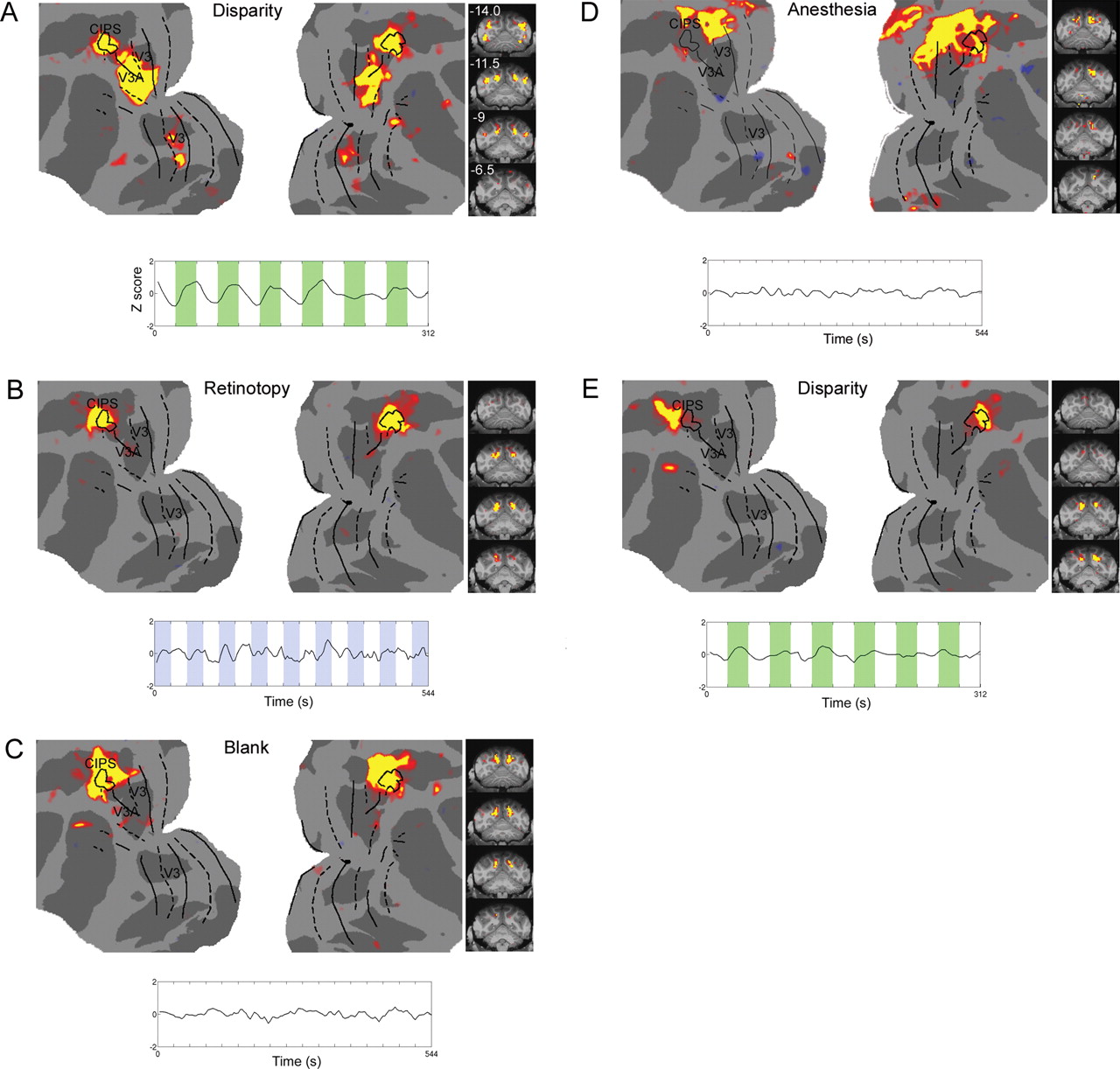
As already mentioned, CIPS is an area highly specialized, along with areas V3 and V3A, for 3D processing (Sakata et al., 1997; Tsutsui et al., 2001; Tsao et al., 2003), and emerged as an IC under multiple visual stimulus conditions (supplemental Fig. S9, available at www.jneurosci.org as supplemental material). Here, we examine in detail the structure of this IC as a function of visual stimulus condition and arousal state. We choose this network for detailed scrutiny because it provides a prominent example of a highly specialized visual network that was reproducibly identified by ICA across stimulus states. ICA of disparity fMRI data revealed an IC comprising areas CIPS, V3, and V3A (Fig. 8A). ICA of retinotopy data also revealed an IC corresponding to CIPS (Fig. 8B), but without V3 and V3A. ICA of blank screen data revealed an IC corresponding to CIPS as well; this IC included additional surrounding cortex within the medial and lateral banks of the posterior IPS (Fig. 8C). ICA of data obtained from an anesthetized monkey revealed an IC that overlapped with CIPS in the right hemisphere; this IC included extensive additional cortex posterior to CIPS within the parieto-occipital sulcus (Fig. 8D). Finally, ICA of disparity fMRI data revealed a second bilateral IC at the base of the intraparietal sulcus, just anterior to CIPS (Fig. 8E). Unlike the IC shown in Figure 8A, this IC was not driven by the disparity stimulus (Fig. 4C; Fig. 8E, time course); rather, it emerged as a discrete, bilateral IC on the basis of correlated spontaneous activity fluctuations. Together, these results underscore that: (1) the spatial structure of networks defined by spontaneous fluctuations does not necessarily correspond exactly to that of networks defined by stimulus-driven fluctuations (contrast Fig. 8A with Fig. 8B,C), (2) the fine structure of networks defined by spontaneous fluctuations can depend on stimulus context (contrast Fig. 8B with Fig. 8C), and (3) a stimulus can induce not only stimulus-locked activity (Fig. 8A), but also correlated spontaneous fluctuations within neighboring regions (Fig. 8E). Such correlated spontaneous fluctuations can be revealed by ICA but not standard GLM analysis.

The CIPS network under different stimulus states. A, Top (identical to Fig. 4D), IC corresponding to V3, V3A, and CIPS, obtained from ICA of fMRI data obtained with a disparity stimulus. Coronal slices covering the activated region are shown on the right (millimeters posterior to the interaural canal indicated in top left corner). Bottom, Time course from this IC, showing activation during disparity epochs. Retinotopic area borders determined by retinotopic localizer experiment (Fig. 4A); CIPS area borders determined by disparity localizer experiment (Fig. 4C). B, Top, IC corresponding to CIPS obtained from retinotopic localizer data. Bottom, Time course from this IC. C, Top, IC corresponding to CIPS obtained from blank screen data. Bottom, Time course from this IC. D, Top, IC corresponding to CIPS obtained from anesthetized data. Bottom, Time course from this IC. E, Top, A second IC obtained from the same data set as in A. Bottom, Time course from this IC shows that this IC was much less strongly modulated by disparity than the IC in A.
Internal temporal structure of ICs as a function of stimulus and arousal state
How does the strength of coupling between voxel pairs within an IC depend on stimulus and arousal state? Supplemental Figure S12 (left), available at www.jneurosci.org as supplemental material, shows the mean temporal correlation between all pairs of voxels in each IC, for three conditions: A) awake, looking at a retinotopic localizer stimulus, B) awake, looking at a blank screen, and C) anesthetized, with eyes shut. As expected, the mean correlation for each IC was always greater than that expected by chance. On the right is plotted the mean temporal correlation between all voxel pairs within an IC as a function of pairwise voxel distance, computed separately for voxels in the left (blue trace) and right (green trace) hemispheres. Data were binned in steps of 1.25 mm. The red trace indicates the mean of the correlations computed from each of the random brain voxel control sets. In the anesthetized case, the pairwise voxel correlation decreased to that expected by random voxel selection, whereas in both awake cases, it remained higher than chance even for separations of up to 2 cm. This suggests that distant regions within a single IC are more strongly functionally connected in the awake brain than in the anesthetized brain.
ICA reveals a highly specific fronto-temporo-parietal network
Most of the ICs identified in our study consisted of bilateral, single-node networks. We found one IC, however, that consisted of six nodes spanning >3 cm of cortex (Fig. 9). The nodes of this IC included subregions of the temporal parietal occipital junction (TPO), dysgranular and granular insula, posterior cingulate, VIP, and dorsal premotor cortex. Although a number of anatomical tracing studies in the macaque have reported connections between subsets of these nodes (Mufson and Mesulam, 1982; Vogt and Pandya, 1987; Morecraft et al., 1993), to our knowledge, this is the first time these nodes have been identified as a functional unit. This IC was observed in one animal in three different sessions, twice with the face localizer stimulus and once with the disparity stimulus. Not all nodes of this IC were activated equally in all three sessions. For example, the insular contribution is most apparent in the first row of Figure 9B, whereas the dorsal premotor contribution is most apparent in the second row. The contributions of TPO and posterior cingulate were strong in all three sessions, suggesting that TPO constitutes a key functional partner of posterior cingulate.

An IC with six nodes. A, Example of network including parts of the TPO, dysgranular and granular insula, posterior cingulate, and dorsal premotor cortex, imaged in two sessions of the face localizer stimulus and one session of the disparity stimulus. Data for three experiments shown on inflated surface. B, Same data shown on slices, from −11 to +20.5 mm relative to the interaural canal.
Discussion
In this study, we set out to systematically partition the macaque brain across different visual stimulus conditions and arousal states using ICA, and then compare the spatial structure of resulting ICs across the different states. We come to three main conclusions: (1) the macaque brain contains a large number of spatially structured independent networks in both the alert and anesthetized state, and ICA is an effective technique for identifying these networks. (2) Many ICs are largely reproducible regardless of the specific visual stimulus (Figs. 5, 6; supplemental Fig. S9, available at www.jneurosci.org as supplemental material), including specialized visual areas (e.g., CIPS), although the fine spatial structure of the IC does depend on the stimulus (Fig. 8). (3) Specific subregions of posterior cingulate, insula, TPO, VIP, and dorsal premotor cortex form a functionally connected network in the macaque brain (Fig. 9).
The effectiveness of ICA for partitioning the macaque brain into statistically independent networks was demonstrated in five ways. First, most ICs were reproducible across independent scan sessions using the same stimulus (Figs. 3, 5, 6; supplemental Fig. S7). Second, for each stimulus and arousal state, ICs collectively covered a large fraction of the scanned brain (Figs. 2, 6, 7). Third, ICA automatically revealed an FEF–LIP network in both alert (Fig. 2) and anesthetized (Fig. 7) animals; this network was previously identified in anesthetized macaques using a seed-based approach that required user input (Vincent et al., 2007). Fourth, when ICA and GLM analysis were applied to the same data set, ICA consistently yielded an IC corresponding to the GLM-identified network (Fig. 4). Finally, ICA revealed in a straightforward manner networks that were not directly driven by any of the sensory stimuli used. These networks included a bilateral network just anterior to CIPS (Fig. 8E), and a network with six bilateral pairs of nodes including parts of the temporal parietal occipital junction, dysgranular and granular insula, posterior cingulate, VIP, and dorsal premotor cortex (Fig. 9). The ability of ICA to reveal previously unsuspected networks makes it an especially powerful exploratory technique, allowing identification of activated areas in situations in which one lacks a model of response time course (precluding GLM approaches) (Duann et al., 2002) or a hypothesis about involved areas (precluding seed-based approaches).
Anesthesia exerted a significant effect on the structure of ICs. The spatial correlation between ICs identified in anesthetized vs alert macaques was substantially lower than that between ICs identified across different visual stimulus contexts (Fig. 7C). Many of the networks obtained in anesthetized macaques spread beyond the borders of corresponding networks in alert animals. For example, under anesthesia, the IC containing MT included the entire STS (Fig. 7D), whereas it was confined to MT proper in awake animals (supplemental Fig. S9A, available at www.jneurosci.org as supplemental material), and the IC containing CIPS included substantial additional cortex within the parieto-occipital sulcus (Fig. 8D). However, it is difficult to draw strong conclusions from comparison of ICs between alert and anesthetized brain states because the manner in which ICA parcellates a particular data set depends on the noise-structure of the fMRI data, and this likely varied substantially between alert and anesthetized states (the former being noisier). Also, it should be noted that these effects may have been due to the specific anesthetic used (ketamine/medetomidine); other anesthetics may exert different effects on functional connectivity. Also, we note that these results do not imply anything about the structure of ICs during natural sleep, which might be a completely different brain state than pharmacologically induced anesthesia.
Compared with anesthesia, stimulus context exerted a more moderate influence on the structure of ICs. A surprising finding of our study was that many visual networks were reproducible not only across independent scan sessions using the same visual stimulus, but also across scan sessions using different visual stimuli (Fig. 5; supplemental Figs. S7, S9, available at www.jneurosci.org as supplemental material), including a blank stimulus (Fig. 6). Stimulus-independent networks included highly specialized regions of visual cortex such as CIPS and MT. Because these areas are known to be driven only by specific visual stimuli, the fact that they emerged as discrete ICs across a large number of different visual stimuli must be attributed to correlated fluctuations in spontaneous activity that were spatially confined to these areas. Networks whose existence depends on stimulus or cognitive state may occur at faster time scales than can be observed with fMRI (Engel and Singer, 2001)
One of the most striking networks revealed by our survey was the highly distributed yet specific network shown in Figure 9. What might the function of this network be? Performance of the fixation task required the monkey to orient spatial attention to the fixation spot in exchange for a juice reward. Because this network includes cortical regions involved in directing spatial attention [posterior cingulate (Olson et al., 1996; Small et al., 2003; McCoy and Platt, 2005), TPO (Smiley et al., 2007), ventral intraparietal area (Schlack et al., 2005)] and processing gustatory rewards [insula (Augustine, 1996)], it may have been involved in orchestrating performance of the fixation task. Alternatively, this network may represent a constitutively active “default mode network” (Raichle and Mintun, 2006). Indeed, it overlaps partially with a putative default network identified by Vincent et al. (2007), although the latter network was much more diffuse. It is noteworthy that the nodes of this network consist of specific subregions of posterior cingulate, insula, TPO, VIP, and dorsal premotor cortex. This suggests that these areas are not uniform in function; rather, specific subregions of one area appear to connect to specific subregions of another to form a functional circuit responsible for accomplishing a specific task (here, fixation). Single-unit recordings guided by task-specific maps of functional connectivity provide a promising approach for dissecting the detailed function of these areas.
Ultimately, to understand the neural basis and functional significance of independent networks identified in fMRI data, it will be necessary to understand their electrophysiological basis, if any. This will require correlating fluctuations in the fMRI signal to simultaneously recorded fluctuations in electrophysiological activity (Logothetis et al., 2001; Goldman et al., 2002; Leopold et al., 2003; Shmuel and Leopold, 2008), and distinguishing fMRI activity that has an electrophysiological basis from fMRI activity driven purely by vascular dynamics (Wise et al., 2004; Schummers et al., 2008; Sirotin and Das, 2009). Such investigations should open new roads into understanding the intrinsic dynamics of the brain. Monkey fMRI experiments provide an important bridge linking cellular investigations into the biophysical basis for intrinsic brain rhythms to explorations of the influence of perceptual and cognitive state on large-scale correlated activity fluctuations.
Footnotes
-
This work was supported by a Sofia Kovalevskaya Award from the Alexander von Humboldt Foundation and by the German Ministry of Science (Grant 01GO0506, Bremen Center for Advanced Imaging). We are grateful to Justin Vincent and two anonymous reviewers for comments on this manuscript, Christian Beckmann for help with MELODIC software, Nicole Schweers for help with animal training and scanning, Ramazani Hakizimana, Nicole Schweers, and Katrin Thoss for expert animal care, and Guerbet for providing Sinerem contrast agent.
- Correspondence should be addressed to Doris Y. Tsao, Broad Institute for Biological Sciences, Caltech, MC 114-96, Pasadena, CA 91125. dortsao{at}caltech.edu


