

Article Figures & Data
Figures
- Figure 1.
Brain slice preparation of AFC and in vivo labeling of contralaterally projecting corticostriatal neurons. A, Schematic depicting retrograde tracer injection in dorsolateral striatum and parasagittal slice angle through the contralateral AFC. B, Epifluorescence (bottom left) and bright-field (top right) images of a coronal brain slice showing the injection site in dorsolateral striatum. D, Dorsal; L, lateral. C, Bright-field image of parasagittal brain slice a with superimposed epifluorescence (Epi) image showing labeled corticostriatal neurons in AFC (arrow). A, Anterior; P, posterior. D, Bright-field (BF) and epifluorescence (Epi) images of AFC of a cKO mouse with layers (L) indicated on the left. WM, White matter. E, Average normalized fluorescence intensity profiles from WT (n = 20) and cKO (n = 10) slices. Cortical depth is shown in normalized units of distance (0, pia; 1, white matter). F, Two-photon microscopy image of three patch-recorded corticostriatal neurons in AFC layer 5. G, Examples recorded from WT (top trace, black) and cKO (bottom trace, red) corticostriatal neurons of APs evoked by depolarizing current injection. H, Plots of average frequency–current (f-I) slope (left) and spike-frequency adaption (SFA) ratios (right), showing no significant differences between WT and cKO. Circles, Data points from individual neurons; line and box, mean ± SEM.
- Figure 2.
Synaptic input mapping in AFC slices. A, Bright-field image showing recording arrangement, including orientation of the 256-site stimulus grid (yellow box), a single stimulus location (*), and the soma of the recorded neuron (triangle). B, Example of EPSC evoked by glutamate uncaging at one stimulus location. C, Array of traces recorded during sequential photostimulation at the 256 sites in the stimulus grid. Responses that were contaminated by direct stimulation of the postsynaptic neuron's dendrites are blank. D, Synaptic input map. Pixel values represent the mean current over a 50 ms poststimulus time window. Black pixels represent traces contaminated by dendritic responses. E, Traces from region of interest (ROI) (gray brackets in D) showing strong layer 2/3 inputs for this neuron. F, Excitation profile. This example shows an AP evoked by perisomatic stimulation of a cKO layer 2/3 pyramidal neuron, recorded in cell-attached mode. The location of the stimulus grid is indicated by the yellow box. G, APs occurred at several locations immediately surrounding the soma. H, Mean distance of AP-generating sites from the soma, an estimator of the spatial resolution of photostimulation (Vexc), did not differ in WT and cKO. Circles, Data points from individual neurons; line and box, mean ± SEM. I, Total number of APs per excitation profile, an estimator of the intensity of photostimulation (NAP), did not differ in WT and cKO. J, Example of a Nissl-stained section of AFC (in a WT mouse). Cells were counted within a 0.1 × 0.2 mm ROI in layer 2/3 (box and inset) to assess relative cell density. K, Number of layer 2/3 neurons per ROI, expressed as cells per 10,000 μm2 in a 50-μm-thick slice (ρcell), did not differ in WT and cKO.
- Figure 3.
Layer 2/3 inputs to layer 5B corticostriatal neurons are stronger in Met-cKO slices. A, Projecting the data in a stack of input maps as an average front view (averaging all the maps) and a side view (averaging along map rows). B, Average WT input maps. White brackets indicate region of interest used for calculating average input. Triangles, Soma positions of the recorded neurons. C, Average cKO input maps. D, Maps of 32 WT neurons projected by averaging along map rows, yielding a side view of the map data set (see A). Each column in the image corresponds to an individual neuron's synaptic input map, averaged along map rows. The data were sorted by the distance of the soma from the layer 5A/B border from highest (closer to pia) to lowest. The vertical white line separates layer 5A neurons (on the left) from layer 5B neurons (on the right). The apparent jitter in soma positions (white triangles) arises from differences in the absolute distances of the layer 5A/B border relative to the pia (gray lines). E, Side view of cKO maps. F, Layer 2/3 input, plotted as a function of the somatic location of the recorded corticostriatal neurons relative to the layer 5A/B border. G, Same data as in F, averaged in 100 μm bins. The asterisk indicates statistically significant difference between groups. H, Input maps for corticostriatal neurons in upper layer 5B. I, Input map obtained by subtracting the WT from the cKO maps in H.
- Figure 4.
Similarity of Met-heterozygous and Met-cKO circuits. A, Bright-field and fluorescent images of retrogradely labeled corticostriatal neurons in the AFC of a HET mouse. B, Average laminar fluorescence intensity profile for HET slices (n = 10); data for WT slices (from Fig. 1) are shown for comparison. C, Side view plot of 33 corticostriatal input maps recorded in HET slices. D, Layer 2/3 input strength plotted as a function of the sublayer location of the corticostriatal neurons (distance of the soma from the layer 5A/B border). E, Average amplitude of layer 2/3 input to layer 5A and 5B corticostriatal neurons in WT, HET, and cKO. Asterisks indicate significant differences (p < 0.05, t test).
- Figure 5.
Unitary connectivity is increased in Met-cKO. A, Bright-field image of slice showing paired recording arrangement. B, Example of connection from a layer 2/3 neuron to a layer 5B corticostriatal neuron in a cKO slice. C, Overall connection probability (pcon). D, Mean uEPSC amplitude for connected pairs (icon). Circles, Data points from individual neurons; line and box, mean ± SEM. The asterisk indicates significant difference (p < 0.05, t test). E, Mean connection amplitude for all pairs (Icon). F, Average paired-pulse ratio (PPR), calculated as the amplitude of the first, second, or third uEPSC relative to the first, did not differ in WT (black) and cKO (gray).
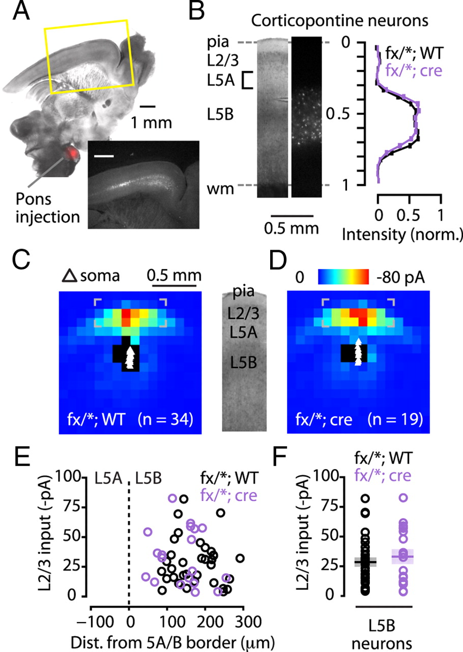
- Figure 6.
Local circuit strengthening in Met-cKO mice does not occur for corticopontine projection neurons in the AFC. A, Retrograde labeling of corticopontine neurons. A red fluorescent tracer was injected into the pons and cerebral peduncle. Inset, Epifluorescence image of labeled corticopontine neurons in AFC layer 5B. B, Laminar distribution of corticopontine neurons. Example bright-field and epifluorescence images (left) and average fluorescent intensity profiles (right) for Metfx/*/WT (n = 13 mice) and Metfx/*/Emx1cre: (n = 8) mice are shown. C, D, Front-view average maps of Metfx/*/WT (n = 34) and Metfx/*/Emx1cre (n = 19) corticopontine neurons show that both groups received layer 2/3 inputs (bounded with gray brackets). E, Layer 2/3 input plotted as a function of the somatic location of the recorded corticopontine neurons relative to the layer 5A/B border. All the corticopontine neurons are in layer 5B. F, Synaptic input from layer 2/3 (averaged over the region of interest indicated by the brackets in C and D) to layer 5B corticopontine neurons recorded in slices prepared from Metfx/*/WT and Metfx/*/Emx1cre mice (p > 0.05, t test). Circles, Data points from individual neurons; line and box, mean ± SEM.
- Figure 7.
Schematic summary of the main microcircuit changes in Met-cKO. Left, The main microcircuits in AFC of WT mice involve connections from layer 2/3 pyramidal neurons (green) to corticostriatal (red) and corticopontine (blue) neurons in layer 5A and 5B. Right, In Met-cKO and HET mice, hyperconnectivity in the excitatory microcircuit from layer 2/3 pyramidal neurons to layer 5B corticostriatal neurons is indicated by filled triangles and thicker arrows. Corticostriatal neurons participate in large-scale loops through the basal ganglia, thalamus, and cortex.


