

Abstract
Human stereopsis can operate in dense “cyclopean” images containing no monocular objects. This is believed to depend on the computation of binocular correlation by neurons in primary visual cortex (V1). The observation that humans perceive depth in half-matched random-dot stereograms, although these stimuli have no net correlation, has led to the proposition that human depth perception in these stimuli depends on a distinct “matching” computation possibly performed in extrastriate cortex. However, recording from disparity-selective neurons in V1 of fixating monkeys, we found that they are in fact able to signal disparity in half-matched stimuli. We present a simple model that explains these results. This reinstates the view that disparity-selective neurons in V1 provide the initial substrate for perception in dense cyclopean stimuli, and strongly suggests that separate correlation and matching computations are not necessary to explain existing data on mixed correlation stereograms.
SIGNIFICANCE STATEMENT The initial step in stereoscopic 3D vision is generally thought to be a correlation-based computation that takes place in striate cortex. Recent research has argued that there must be an additional matching computation involved in extracting stereoscopic depth in random-dot stereograms. This is based on the observation that humans can perceive depth in stimuli with a mean binocular correlation of zero (where a correlation-based mechanism should not signal depth). We show that correlation-based cells in striate cortex do in fact signal depth here because they convert fluctuations in the correlation level into a mean change in the firing rate. Our results reinstate the view that these cells provide a sufficient substrate for the perception of stereoscopic depth.
Introduction
Stereoscopic vision is possible because objects that are at a different depth from the point of fixation will project to different locations on the left and right retinae. However, to successfully infer depth, the brain must first match elements in the left and right eyes, which correspond to the same object. This computationally demanding task is known as the stereo correspondence problem, and is particularly challenging in dense “cyclopean” stimuli like random-dot stereograms (RDS; Julesz, 1971; Marr and Poggio, 1976).
Binocular processing starts in area V1, where neuronal responses are well described by the binocular energy model (BEM; Ohzawa et al., 1990; Cumming and Parker, 1997), which carries out a computation closely related to binocular cross-correlation (Qian and Zhu, 1997; Allenmark and Read, 2011; Henriksen et al., 2016b). One hallmark of this computation is that inverting the contrast in one eye should also invert the profile of the disparity-tuning curve. Although this is true of disparity-selective neurons (Ohzawa et al., 1990; Cumming and Parker, 1997; Nieder and Wagner, 2000), they typically show weaker modulation to anticorrelated stimuli than to correlated stimuli (Cumming and Parker, 1997; Qian and Zhu, 1997). Thus, these responses do not exactly represent binocular cross-correlation, but seem to be correlation-based. Nonetheless, the success of the BEM in describing both neuronal responses and psychophysical properties of stereopsis has led to the widespread view that stereo correspondence begins with a correlation computation (Ohzawa et al., 1990; Cumming and Parker, 1997; Qian and Zhu, 1997; Banks et al., 2004; Filippini and Banks, 2009; Allenmark and Read, 2011; Kane et al., 2014).
However, a series of recent publications by Doi et al. (2011, 2013, 2014) has suggested that a quite different computation is needed for some stimuli because humans are able to see depth in RDS constructed with an equal number of correlated and anticorrelated dots (termed half-matched RDS; Doi et al., 2011, 2013; Doi and Fujita, 2014). The stimulus is illustrated in Figure 1. These stimuli have a mean binocular correlation of 0 (because the correlation of the correlated and anticorrelated dots cancel out) and therefore many correlation-based computations, such as the binocular energy model, do not signal disparity here. This led Doi et al. (2013) to propose that an additional “matching computation,” possibly performed in extrastriate cortex, accounts for human depth perception in dense half-matched random-dot stereograms. If V1 neurons only perform a correlation computation, then this observation implies that humans see depth in half-matched stereograms even though V1 neurons do not signal disparity in their mean firing rate. This would be surprising as V1 activity is generally thought to be a necessary prerequisite for cyclopean depth perception. Indeed, it would provide the first evidence that depth perception can occur without an explicit signal in V1.

Illustration of a random dot stereogram. Black and white dots are painted in the left and right image with disparity applied to the dots. Top row, All the dots have the same contrast in the left and right eyes and so the stereogram is binocularly correlated. Middle row, All the dots have opposite contrast in the two eyes (black is matched with white, and vice versa), and so the stereogram is anticorrelated. Bottom row, The stereogram has an equal number of correlated and anticorrelated dots, and so the stimulus is half-matched.
Thus, the current literature on half-matched stereograms suggests a radical change in our understanding of the role played by area V1 in depth perception. This argument depends critically on the assumption that V1 neurons perform a correlation computation, as described by the binocular energy model. However, the attenuated responses to anticorrelated RDS already indicate that disparity selective responses in V1 do not simply reflect correlation. This raises the possibility that neurons in V1 do modulate their firing rate with disparity in half-matched stereograms. We therefore investigated the responses of disparity-selective cells in macaque V1 to half-matched random-dot stereograms. We find that these cells do signal disparity (weakly) in the half-matched condition. A simple model that exploits local fluctuations in correlation can explain this finding, and also predicts that the strength of disparity tuning for half-matched stimuli should decrease with increasing dot density. We show that variation in dot density does have this effect on the responses of V1 neurons. The observed responses to half-matched stereograms restore the view that disparity-selective neurons in V1 provide a sufficient substrate for depth judgments in random-dot patterns. The effects of dot density suggest that a simple mechanism can explain these responses.
Materials and Methods
Animal subjects.
Two male macaque monkeys (subjects Lem and Jbe) were implanted with head posts, scleral search coils, and a recording chamber under general anesthesia. The full experimental procedure is described in detail previously (Cumming and Parker, 1999; Read and Cumming, 2003). Briefly, subjects viewed separate CRT monitors with each eye through a mirror haploscope. They were required to fixate a bright spot on each CRT, and maintain fixation for 2.1 s to earn a drop of liquid reward. The window of fixation was typically a box of 0.8° × 0.8° around the fixation spot. One subject was trained to perform a front/back discrimination task with random-dot patterns as described by Prince et al. (2000). All experiments were performed at the US National Institutes of Health. All procedures were performed in accordance with the US Public Health Service policy on the care and use of animals. The protocols were approved by the National Eye Institute Animal Care and Use committee.
Model cells.
The model cells were constructed exactly as described by Henriksen et al. (2016a) using BEMtoolbox, a MATLAB toolbox for simulating binocular energy model cells (available at https://www.github.com/sidh0/BEMtoolbox). In brief, the BEM models a complex cell by combining the responses of two binocular simple cell subunits. The simple cell has linear monocular receptive fields (RFs) described by a Gabor function. For simplicity, here we used identical RFs in the two eyes, so that model cells have a preferred disparity of zero. The responses from left and right RFs are summed and then squared. A binocular complex cell is the sum of two simple cells in quadrature, ie, with RF phase differing by π/2. We modeled a cell whose response was a nonlinear function of correlation by including a static squaring output nonlinearity. Thus, the final model is simply as follows:
 where S12 and S22 are the two simple cell subunits of the BEM model. We computed the mean response of the model to correlated, half-matched and anticorrelated random-dot stereograms at 5% and 24% dot density. Twenty-one disparities were used, evenly spaced between −0.5° and 0.5°. The model response was averaged across 10,000 presentations for each stimulus condition.
Recording.
We recorded extracellular activity from cells in V1 using 24-channel linear multi-contact electrodes (V-probes, Plexon), with 50 μm spacing between the probes. Behavioral and neuronal data were sampled using Spike2 (Cambridge Electronic Design). The spike waveform data were saved to disk for offline analysis, and spikes were classified offline using custom software. Cells that were well isolated and exhibited significant disparity tuning to correlated random-dot stereograms of both 5% and 24% density as determined by a one-way ANOVA (p < 0.01) were included in the analysis. Fifty-three of 90 cells passed these criteria.
Stimulus.
Black and white square dots were painted on a gray background, with disparity applied to the center of the stimulus, keeping a zero-disparity annulus as reference (to eliminate monocular cues; without a zero-disparity annulus, the observers might be able to detect a monocular shift in the dot pattern from trial-to-trial). The stimulus is illustrated in Figure 1. For recordings from the operculum (relatively foveal with RF eccentricity 1–3.5°), the disparity-defined region was 3.4° in diameter, whereas the surrounding annulus had a width of 1°. The annulus had a disparity of 0° and a correlation that matched the center. Some recordings were made from neurons in the calcarine sulcus by advancing the probe through the operculum. For these recordings (eccentricities 10–13°), the disparity-defined region was 4.2 deg in diameter, whereas the annulus had a width of 2°. This was done to ensure that the larger RFs in the calcarine were completely covered by the disparity-defined region. For half-matched stimuli, we painted an equal number of correlated and anticorrelated dots. Each dot had an equal probability of being black or white. An illustration of this stimulus is shown in Figure 1. Disparity values were chosen based on disparity tuning curves collected before the experiment, ensuring that the range over which cells exhibit disparity tuning was covered in our selection of disparity values. Each cell was tested with at least nine, sometimes as many as 16, disparities. The random-dot stereograms were presented dynamically at a pattern refresh rate of 100 Hz. Each dynamic RDS stimulus was presented for 420 ms (ie, consisting of 42 unique dot patterns), with four stimuli being presented in a given trial with a 100 ms gap (gray screen) between the stimuli. Thus, four stimuli were presented in each completed fixation trial (2.1 s). This allows four stimulus presentations to be completed while only rewarding the monkey once. Because we anticipated weak responses to the half-matched stimuli, they were presented 10 times more frequently than correlated or anticorrelated disparities. On average each correlated (or anticorrelated) stimulus was shown 16 times, whereas each half-matched stimulus was shown on average 161 times. We used two dot density values, 5% and 24%, where dot density is defined as the percentage of the stimulus area that the dots would occupy if they did not occlude one another. The dots were, however, allowed to occlude, but were painted in random order so that correlated dots did not systematically occlude anticorrelated dots or vice versa, and so that the center did not systematically occlude the surround or vice versa. For the electrophysiological experiments, the monkey simply needed to maintain fixation. The dot size varied depending on the size of the RF. Previous modeling work has shown that the ratio between receptive field size and dot size may affect the magnitude of half-matched responses (Henriksen et al., 2016a). Thus, for eccentric recordings (defined as >10° eccentricity), the dot size was increased to 0.2 or 0.3° to compensate for the larger RFs (3 sessions, 19 cells). In the remaining recordings, the dot size was 0.1° (9 sessions, 34 cells).
To provide quantitative estimates of RF size, we measured responses to thin strips of random dot texture. Vertical strips were placed at a variety of horizontal positions, spanning the RFs of all recorded neurons, and a Gaussian function of position (SD σx) was fit to the spike counts. Horizontal strips were used to estimate size in the vertical direction (SD σy). RF size was then defined as
For neurophysiology experiments, stimuli were presented on two Viewsonic P225f CRT displays, with a resolution of 1280 × 1024 at 100 Hz. At the viewing distance used (89 cm) each pixel subtended 0.018°. The luminance response was measured with a Konica-Minolta LS100 photometer, and linearized with a lookup table. The mean luminance was 40 cd/m2, and contrast was >99%.
Quantifying disparity tuning.
To quantify correlated disparity tuning, we used a standard metric known as the disparity discrimination index (DDI; Prince et al., 2002). The DDI was computed using the square root of the firing rate to ensure equal variances for different disparities/firing rates. The DDI is defined as follows:
 where Rmax and Rmin correspond to the maximum and minimum mean square root firing rates on the tuning curve, and RMSerror is the root mean square error around the mean square root rates in the tuning curves. The DDI gives a measure of how large the peak-to-trough difference in the tuning curve is relative to the intrastimulus variability. A DDI near 0 thus means that the cell can poorly discriminate the disparities corresponding to the peak and trough of the disparity-tuning curve. The DDI approaches 1 as the variability becomes negligible relative to the response range.
To quantify disparity tuning to half-matched stimuli, we computed the regression slope between correlated and half-matched responses (type 2 regression; Draper and Smith, 2014). The half-matched regression slope estimates the magnitude of disparity tuning to half-matched stimuli as a fraction of that for correlated stimuli. A half-matched slope of 1 would mean that the cell has the same disparity tuning to half-matched stimuli as it has to correlated stimuli; a half-matched slope of 0 would mean either that the cell shows no disparity tuning to half-matched stimuli or that the half-matched tuning is present but has a shape that is uncorrelated with the correlated tuning. We observed no instances of the latter, so we used the slope as an index of response magnitude. We also quantified the anticorrelated disparity tuning equivalently by computing the regression slope between the correlated and anticorrelated responses. If the cells modulated their firing rate strictly as a linear function of correlation, the anticorrelated slope should be −1 (corresponding to an amplitude ratio of 1 and a phase change of π). The anticorrelated slope is closely related to the anticorrelated amplitude ratio that has been previously used (Cumming and Parker, 1997). The amplitude ratio uses the amplitude of Gabor functions fitted to each of the tuning curves, which has the advantage that it can capture a broader range of changes in the tuning curve, such as phase shifts other than 0 or π. However, because the ratio must exceed 0, it can overestimate weak modulation, which the slope estimate used here does not. We obtained confidence intervals for the half-matched and anticorrelated slopes by resampling of residuals (Efron and Tibshirani, 1994). For each cell and stimulus dot match value, we performed a square-root transform on the spike counts, before computing the (square-root transformed) residuals for each disparity. To construct a single resampled disparity-tuning curve, we drew a sample from the pool of residuals, added this on to the square root of the mean firing rate, and squared the value. This gave us one resampled trial. We repeated this for ki trials, where ki is the number of trials (observations) for the ith disparity value. To generate half-matched slope confidence intervals, we generated a resampled tuning curve for correlated data, and a resampled tuning curve for half-matched data, and then computed the slope between the two. We repeated this procedure 100,000 times, and obtained the 95% confidence intervals for the slopes. The corresponding procedure was done for anticorrelated data to obtain confidence intervals for anticorrelated slope.
ROC analysis.
The ROC curve traces the performance of a binary classifier by plotting the false-positive rate versus the true-positive rate using a variable threshold; in this case the classifier is a cell's ability to discriminate preferred disparity trials from null disparity trials (Green and Swets, 1966; Tolhurst et al., 1983; Britten et al., 1992). For each cell, we chose the two disparities with the largest and smallest mean response in response to correlated RDS (ie, preferred and null disparities). Using the half-matched responses to these disparities, we computed the true and false-positive rates by progressively incrementing the classification threshold. This gives us the ROC curve for an individual cell. To obtain neurometric performance for the cells to half-matched stimuli, we computed the area under the receiver operating characteristic curve (AUROC). The AUROC varies from 0 to 1. A value of 0 means that the classifier is always incorrect, whereas a value of 1 means that the classifier is always correct. An AUROC value of 0.5 corresponds to chance performance. Thus, the AUROC as a measure of neurometric performance is equivalent to percentage correct as a measure of psychometric performance.
The tuning curves we have collected are available at https://www.github.com/sidh0/hm with an accompanying interactive data browser written in MATLAB. MATLAB code for generating all figures in the current paper is also available on the Github repository.
Results
Model disparity-tuning curves
We have previously shown that a simple modification to the binocular energy model can produce disparity selectivity for half-matched stimuli (Henriksen et al., 2016a), by adding a squaring nonlinearity at the output of a traditional binocular complex cell. The result is that positive binocular correlation produces a larger change in activity than negative correlation of the same magnitude. This in turn means that random fluctuations in correlation around a mean of zero produce a larger response than a correlation that is fixed at zero. (This is because the expected value of a squared random variable depends on its variance: E(X2) = [E(X)]2 + Var(X), so that the squaring output nonlinearity makes the mean firing rate depend in part on the variance in binocular correlation). The original binocular energy model does not signal depth in half-matched stereograms because its response varies linearly as a function of binocular correlation. Thus, when the mean binocular correlation is zero, the mean response of the model is equal to its uncorrelated response (although the variability of the response is greater in the half-matched case; Doi et al., 2013; Doi and Fujita, 2014; Henriksen et al., 2016a). The extent of this variation in binocular correlation will depend on the number of dots contained within the receptive field. More dots within the receptive field reduce the fluctuations in correlation. If dot density (expressed in the fraction of pixels that are covered by dots) is held constant, smaller dots produce more dots in the receptive field. For fixed dot size, higher density also increases the number of dots. Thus, small dots and high dot density both reduce the fluctuation in correlation over the receptive field. Consequently, the Var(X) term is smaller, and the mean response of the cell is lower. Decreasing the dot size and increasing the RF size are functionally equivalent operations; thus, both produce the same decrease in the fluctuations in the correlation level seen by the cell. In Figure 2 we show the effect of dot density on disparity tuning by plotting the responses of the model neuron described in (Henriksen et al., 2016a) to random dot patterns of two densities. We computed disparity tuning curves in response to correlated, half-matched and anticorrelated random-dot stereograms. We used two dot densities, 5% and 24%. Figure 2a shows the response of the model to 5% dot density stimuli. The tuning curves to correlated and anticorrelated stimuli are asymmetric due to the output nonlinearity. For the half-matched stimuli, the model cell exhibits clear disparity tuning at the preferred disparity of the cell. At higher dot densities (Fig. 2b) the half-matched disparity tuning, although still present, is greatly attenuated relative to the 5% density stimuli. Thus, our model predicts that there should be a correlation between the magnitude of half-matched tuning to 5% and 24% density reflecting variation between cells in, for example, the output nonlinearity. It also predicts that the responses to the higher dot density should show weaker modulation. One simple way to appreciate these results is to consider a dot density so low that only one dot ever falls within the RF. One-half of the stimuli will be 100% correlated, and one-half will be 100% anticorrelated. The cell's response will then be the mean of its responses to correlation and anticorrelation. As density is increased, the fluctuations in correlation are reduced, and the disparity-related response of the cell weakens.

Disparity tuning curve of a model cell which signals disparity in half-matched stimuli. In a, the density of the stimulus was 5%, whereas in b the density was 24%. The inset shows a magnified view of the response to half-matched stereograms. The model cell is simply a traditional binocular energy model with an additional squaring nonlinearity on the output (Henriksen et al., 2016a). Increasing the dot density decreases the local correlation variability and thus decreases disparity tuning to half-matched stimuli. b, Inset, A zoomed-in view of the half-matched tuning curve. Each point in a given tuning curve was generated by averaging the responses of the model cell to 10,000 unique dot patterns.
Neuronal responses
We recorded extracellular activity of 53 isolated disparity-selective V1 neurons in response to correlated, anticorrelated and half-matched dynamic random-dot stereograms, while two macaque monkeys maintained fixation. We used two dot densities, 5% and 24%, to test the model predictions that the magnitude of disparity tuning to half-matched stimuli should decrease with increasing dot density. Figure 3a shows an example disparity tuning curve for a cell in response to 5% dot density stimuli. As in the model, this cell has asymmetric correlated and anticorrelated tuning curves and a peak in its response to half-matched stereograms at the preferred disparity of the cell. In response to 24% dot density stimuli (Fig. 3b), the cell's half-matched tuning decreases visibly, whereas the correlated and anticorrelated responses remain largely unchanged.

Example tuning curves for a cell that is selective for disparity in dynamic half-matched stimuli for both 5% dot density (a) and 24% dot density (b) stimuli. Dot width was 0.3°, and RF width was 1.05°. b, Inset, A zoomed in view of the half-matched response. No inset is shown for a because the response is sufficiently large to see unaided. Error bars show ±1 SEM. The bottom shows the half-matched and anticorrelated responses plotted as functions of the correlated response for 5% density (c) and 24% density (d). Lines show type 2 regression fits. 95% bootstrap CIs for half-matched slope was (0.197, 0.27) for 5% density, and (0.076, 0.125) for 24% density. For anticorrelated slope, the confidence intervals were (−0.591, −0.45) for 5% density and (−0.637, −0.492) for 24% density.
To quantify the magnitude of disparity tuning to half-matched and anticorrelated stimuli relative to the correlated response, we computed the regression slope between the correlated and half-matched responses (half-matched slope) and between the correlated and anticorrelated responses (anticorrelated slope). Figure 3, c and d, shows this for the 5% and 24% density stimuli, respectively.
In the example cell shown in Figure 3, the anticorrelated slope is ∼0.5 for both densities tested. This is typical: across the population, anticorrelated slopes did not differ significantly for 5% versus 24% density (t(52) = 0.97, p = 0.34, paired t test). In contrast, half-matched slopes do depend on dot density. The half-matched slope in the low density case is 0.23 [95% bootstrap CI (0.197, 0.27)], meaning that the magnitude of half-matched disparity tuning is 23% of that for correlated disparity. In the high density case, the half-matched slope is 0.1 [95% CI (0.076, 0.125)], or 10% of the correlated tuning. In other words, the strength of disparity tuning has approximately halved in response to increasing the dot density (ie, decreasing the correlation variability), yet remains significantly >0.
Figure 4 summarizes this result across the population, showing the half-matched slope as a function of disparity tuning strength, which is quantified with the DDI. The DDI ranges from 0 to 1 and is a measure of a cell's disparity tuning (Prince et al., 2002). Figure 4a shows that there is no significant correlation between the DDI and the half-matched slope of a cell for low density (r = −0.02, p = 0.91, Pearson correlation), and only a modest relationship between DDI and half-matched slope in the high density stimuli (Fig. 4b; r = 0.34, p = 0.01, Pearson correlation). This latter observation might reflect the higher signal-to-noise ratio in neurons with higher DDIs. Under the null hypothesis that V1 cells are, on average, not tuned to disparity in half-matched stereograms, the distribution of half-matched slope values should be centered on 0. In Figure 4 the mean half-matched slope is significantly greater than zero for both densities (5%: M = 0.14, t(52) = 11.46, p < 10−15; 24%: t(52) = 6.76, p < 10−7). This is also true for both subjects when we consider their data separately (Lem 5%: M = 0.14, t(27) = 8.75, p < 10−8; Lem 24%: t(27) = 4.55, p < 10−3; Jbe 5%: M = 0.14, t(24) = 7.33, p < 10−6; Jbe 24%: M = 0.04, t(24) = 5.35, p < 10−4). Neurons that exhibit significant disparity-tuning to half-matched stimuli are shown as red triangles, whereas those that did not are shown as green circles. For low dot density stimuli (Fig. 4a), 34/53 cells exhibit significant half-matched disparity tuning, whereas for high dot density stimuli (Fig. 4b), 11/53 cells show significant tuning. Thus, on average, V1 neurons transmit a systematic disparity signal even in 24% density half-matched RDSs.

Half-matched slope (ie, the regression slope of responses to half-matched stimuli as a function of the responses to correlated stimuli) plotted as a function of DDI for correlated stereograms for 5% density (a) and 24% density (b). The red triangles show cells that exhibit significant disparity tuning to half-matched stimuli at the p < 0.01 level (a, 34/53 cells; b, 11/53 cells). The blue square shows the example cell in Figure 3. The dashed black line shows the expected half-matched slope under the null hypothesis that V1 cells are not, on average, disparity-tuned to half-matched stimuli. In both plots the points deviate significantly from this prediction.
As noted above, our model predicts that there should be a correlation between the magnitude of half-matched tuning at different dot densities. We do find a moderate correlation between the half-matched slopes at 5% and 24% density (r = 0.43, p = 0.001, Pearson correlation). Our model also predicts that half-matched tuning should be weaker for stimuli with higher dot density, since these have smaller fluctuations about the mean correlation level of zero. The difference between the 5% and 24% density slopes is indeed highly significant (M = 0.14 for 5% vs M = 0.04 for 24%, t(52) = 9.51, p < 10−12, paired t test). This was also true for both monkeys when considered separately (M = 0.14 for 5%; M = 0.04 for 24% density; p < 10−6 in both cases).
In our simple model, the magnitude of disparity selective responses depends on the dot size, the dot density, and the receptive field size, because all of these things alter the local variation in correlation (Henriksen et al., 2016a). Despite this, the model predicts a unique relationship between the slope of responses to half-matched versus correlated stimuli observed at 5% density and that at 24% density. Two different combinations of RF size and dot size that produce the same slope at 5% density will also produce the same slope at 24% density. This arises because the only factor that determines the response magnitude for half-matched stimuli relative to correlated stimuli is the variance in local correlation (other factors, such as contrast or spatial frequency content would affect responses to both stimuli equally). Importantly, this means that the model predicts the relationship between slopes (as a function of density) without any fitting of parameters. We show this expected relationship between the half-matched slope for the two dot densities in Figure 5 (red line). Although there may be a deviation at large slope values (>0.3), we have too few neurons with these responses to be clear that this really is a model failure. As a result, over the observed range, the quantitative success of the model is mainly in describing the mean slope magnitudes, rather than the shape of any relationship. Nonetheless, since the model prediction was made without any parameter fitting, this success provides strong evidence that V1 cells signal disparity in these stimuli by exploiting fluctuations in local correlation within the RF. Note that if responses to half-matched stimuli represented a contribution from a pure “matching computation” (Doi et al., 2011, 2013; Abdolrahmani et al., 2016; Henriksen et al., 2016a), the data in Figure 5 should lie on the identity line, which they do not.
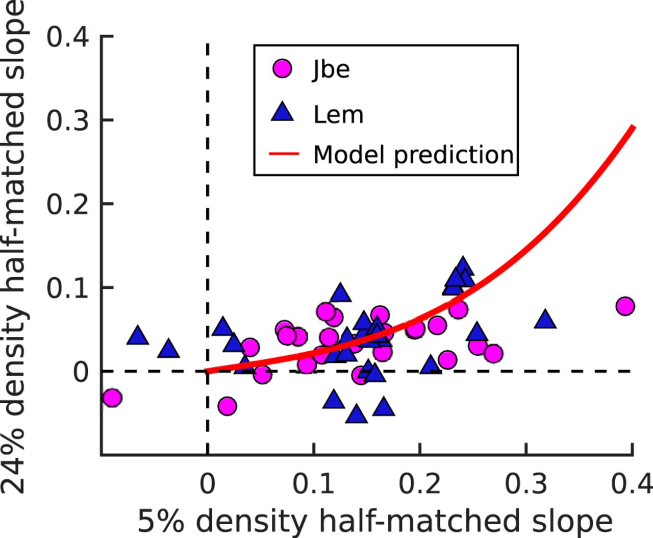
Comparing half-matched disparity tuning for two dot densities (5% and 24%). Tuning strength is quantified with the half-matched slope. Data are shown from 53 cells. Blue triangles show data from monkey Lem, whereas magenta circles show data from monkey Jbe. The solid red line shows the prediction of the modified binocular energy model introduced earlier (with no free parameters). The model prediction was obtained by computing the 5% and 24% density responses of model cells with different RF sizes.
Testing more general models of a single mechanism
The quantitative prediction shown in Figure 5 is specific to our particular model: the binocular energy model with a squaring output nonlinearity. However, for a wide range of models in which a cell's half-matched response reflects its averaged response to positive and negative fluctuations in binocular correlation, there should be a relationship between a cell's attenuation to anticorrelated stimuli and the magnitude of the half-matched tuning. We assess the attenuation using the anticorrelated slope (ie, the gradient of the regression line when anticorrelated responses are plotted against correlated). In neurons where responses to anticorrelation shows no attenuation, the mean response to a mixture of correlations with a mean of zero is the same as the response to zero correlation, and so a straightforward prediction is that there should be no tuning for half-matched stimuli: the half-matched slope should be zero when the anticorrelated slope is −1. As the modulation to anticorrelated stimuli gets weaker, this averaging allows fluctuations in correlation to produce stronger responses to half-matched stimuli at the preferred disparity (although responses to half-matched stimuli will always be near-zero when fluctuations are small, eg, if receptive fields are large compared with dot size (Henriksen et al., 2016a). Thus, the range of possible half-matched slopes should be maximal when the anticorrelated slope is zero (or positive).
In the low density stimuli (Fig. 6a), there is some support for this. There is a weak positive correlation between the two (r = 0.25, p = 0.07, Pearson correlation), although this marginally fails to reach significance. For high densities (Fig. 6b), this trend is not evident or even reversed (r = −0.21, p = 0.13, Pearson correlation). However, there are a number of reasons why this relationship may be obscured. For example, receptive field size affects half-matched slope without affecting anticorrelated slope. Additionally, because the half-matched slopes are all small, it may require considerably more statistical power to reveal any relationship. We have sufficient power to demonstrate that these cells are on average disparity tuned to half-matched RDSs at 24% density, but not for more sophisticated analyses.

Half-matched slope as a function of anticorrelated slope for 5% density (a) and 24% density (b). The blue square shows the example cell in Figure 3 and the magenta square shows the example cell in Figure 7. If the half-matched response can be inferred from the correlated and anticorrelated responses alone, then there should be a positive correlation between half-matched and anticorrelated slope (ie, less attenuation to anticorrelation would imply smaller half-matched slope). Although there is a trend bordering on significance for low-density (a), no such relationship is evident in the high-density stimuli (b). The red and blue crosses show the expected performance of idealized correlation and matching computations, respectively.
In Figure 6, the red and blue crosses show the predictions of idealized correlation and matching computations, respectively. A pure correlation computation, such as the BEM, would have perfectly inverted response to anticorrelated, and consequently no response to half-matched (anticorrelated slope of −1, half-matched slope of 0). A pure matching computation would not modulate its response at all to anticorrelated dots, but would have a half-matched amplitude which is half its correlated amplitude (anticorrelated slope of 0, half-matched slope of 0.5). This is clearly not a veridical characterization of the neurophysiological data, which shows instead a cloud centered in between these two extremes, and which changes with stimulus parameters, such as dot density. This is consistent with the view that disparity tuning in V1 arises from a single nonlinear correlation computation, which can be roughly approximated by appending a squaring on to the BEM.
Many neurons in Figure 6 have anticorrelated slopes near 0 or even greater than zero, suggesting there may be a subpopulation of neurons with no disparity-selective response to anticorrelated dots, which seems at odds with the observations by Cumming and Parker (1997). This apparent discrepancy reflects two factors: first, some neurons do show clear modulation to anticorrelated stimuli but without any inversion. Some show tuning of similar shape [these are shown with phase shifts near 0 by Cumming and Parker (1997), and have slopes >0 here], and some show shapes that differ in other ways (phase shifts neither 0 or π). Second, random fluctuations in a neuron showing no systematic response will produce slope values scattered around zero here, but inevitably produce amplitude ratios >0 when using fitted Gabor functions.
A less stringent version of the model prediction in Figure 5 is that the response to half-matched stimuli should be less than or equal to the average of the correlated and anticorrelated responses. Only one cell in our dataset deviated significantly from this prediction. This cell, shown in Figure 7a for 5% density, shows completely symmetric tuning curves to correlated and anticorrelated stimuli (ie, an anticorrelated slope not significantly different from −1), yet has a half-matched slope of 0.14 [95% CI (0.103, 0.173)]. In other words, this cell's response to half-matched stimuli is greater than that predicted from the average of its correlated and anticorrelated responses. For 24% density stimuli (Fig. 7b), the cell has an anticorrelated slope that is significantly <−1, yet its half-matched slope is again significantly positive [95% CI (0.005, 0.06)]. This means that the cell's half-matched tuning is opposite to that produced by a random mixture of responses to correlated and anticorrelated stimuli. These responses are rare, so it is possible that these cells process disparity in a way that is different from other cells in striate cortex. Alternatively, it may be that our model is too simple to fully describe the behavior of V1 neurons, a point we return to in the discussion. Nonetheless, in 52/53 neurons, the 95% confidence interval for the half-matched slope included the value predicted by the model.

An unusual example cell that exhibits significant disparity tuning to half-matched stimuli despite having symmetric tuning curves to correlated and anticorrelated dot-patterns. a, b, The tuning curves for 5% and 24% density dot-patterns, respectively. Error bars show ±1 SEM. 95% bootstrap confidence intervals for the half-matched slope was (0.103, 0.173) for 5% density and (0.005, 0.06) for 24% density. The corresponding confidence intervals for anticorrelated slope was (−1.147,−0.876) and (−1.319,−1.066) for 5% and 24%, respectively. To 24% density stimuli (b), the cell has an anticorrelated slope that is significantly <−1 yet still exhibits significant disparity-tuning to half-matched stimuli. a, b, Insets, A zoomed in view of the half-matched response. The bottom shows the half-matched and anticorrelated responses plotted as a function of the correlated response for 5% and 24% density (c and d, respectively).
Neurometric performance
The analysis above demonstrates that neurons in V1 do carry a weak but systematic signal about disparity in half-matched stereograms. This analysis does not demonstrate whether the disparity tuning is sufficient to account for psychophysical behavior. We chose our high density (24%) because that value has been used in previous psychophysical studies (Doi et al., 2011, 2013; Henriksen et al., 2016a). If the weak tuning to half-matched stimuli we find with this density is not sufficient to account for psychophysical performance, it might be necessary to postulate a separate matching computation, as hypothesized in the literature (Doi et al., 2011, 2013; Doi and Fujita, 2014). To evaluate neuronal performance, we computed the neurometric performance of the cells using the AUROC. The ROC curve was computed for each cell by comparing responses to its preferred disparity (ie, the disparity where the cell had the highest mean firing rate) and responses to its null disparity (ie, disparity with lowest mean firing rate). Preferred and null disparities were defined on the basis of responses to correlated stereograms. The AUROC values are shown in Figure 8a for 5% dot density stimuli and in b for 24% stimuli. This then estimates how reliably an ideal observer could discriminate a half-matched stimulus at the preferred disparity from one at the null disparity, given only the spike counts of the neuron. These can then be compared with psychophysical performance, also expressed as percentage correct. The neurometric performance is lower than the published performance of human observers. Human performance is often >80% correct on half-matched stereograms, although there is substantial variability between individuals (Doi et al., 2011, 2013). However, there are a number of important differences between the stimulus conditions used in the psychophysics and that used here. Most importantly, the published human studies used foveal viewing of stimuli that were much larger than typical foveal receptive fields, giving them much more information than any single V1 neuron. We trained one of our animals to perform a discrimination task, and then measured performance by using stimuli matched to those used during recording. For the recording sessions, the stimuli used at a given eccentricity were identical except for small changes in position (necessary to center the stimulus on recorded RFs). The psychophysics used the same stimulus configuration, with the location set to the mean of those used in the recording sessions. The animal performed at 70% correct at the eccentric location and 65% correct at the more foveal location. This stimulus was larger than typical receptive fields (chosen to ensure that the RFs of all cells recorded in a session were covered by the stimulus, even when considering fixational eye movements). We therefore repeated the psychophysical measures changing only the size of the region with disparate dots to match measured RF sizes. (RF size was estimated by the SD of a Gaussian fit to the measures of minimum response field. The stimulus diameter was set to be eight times the mean of these SDs, still more than adequate to cover the RF). Here the animal achieved only 51% correct, poorer than the mean AUROC (and not significantly >50%). Thus, when care is taken to match the information available to individual neurons and the psychophysical observer, the ability of single neurons to detect disparity in half-matched stereograms is sufficient to account for psychophysical performance.

AUROC for all cells for 5% dot density (a) and 24% dot density (b). Red dots show data from more foveal recordings (<5° from fixation), and black dots show data from eccentric recordings (>10° from fixation). Only monkey Lem had eccentric recordings. The AUROC estimates the percentage correct on near/far task that can be achieved using the spike counts from a single neuron (see Materials and Methods).
Discussion
Disparity-selective V1 cells probably provide the initial substrate for binocular depth perception, at least in dense cyclopean stimuli such as RDSs. Disparity-selective cells in V1 appear to carry out a local correlation-based computation, similar to that described by the BEM. Depth perception in half-matched random-dot stereograms, stimuli with an equal number of correlated and anticorrelated dots, has been proposed as evidence that a separate stereo matching computation operates in cortex (Doi et al., 2011, 2013; Doi and Fujita, 2014). This is based on the observation that a computation that modulates its response strictly as a linear function of correlation, such as the BEM, cannot report depth in these stimuli. However, it is well known that disparity-selective cells in V1 often have attenuated responses to anticorrelated stimuli, which is also unlike the BEM. We have previously shown that a simple model that reproduces attenuated response to anticorrelated RDS can also produce disparity selectivity for half-matched RDS (Henriksen et al., 2016a). This raises the possibility that V1 neurons might signal disparity in half-matched stereograms. Here, we show that disparity-selective neurons in primate V1 do show systematic disparity selectivity to half-matched RDSs. These properties suggest that V1 neurons carry out a nonlinear correlation computation, intermediate between a “pure correlation” and “pure matching” computation. We propose that these cells are the initial neuronal substrate for depth perception in half-matched RDS. This nonlinear response to binocular correlation may represent the effect of mechanisms that reduce responses of V1 neurons to “false” matches (Henriksen et al., 2016b).
In the model which prompted this work, this tuning arises from fluctuations in the local binocular correlation within the receptive field. Any stimulus manipulation that decreases the local correlation fluctuations should decrease the magnitude of the model's disparity tuning to half-matched stimuli. In our experiments, we decreased correlation fluctuations by increasing dot density. We found that this reduces half-matched disparity tuning in real neurons, as predicted by the model. It is noteworthy that a number of psychophysical observations suggest that local correlation fluctuations are also required for depth perception (Doi et al., 2013; Henriksen et al., 2016a), providing further evidence that V1 neurons are indeed the neural substrate for the psychophysics.
Doi et al. (2014) have proposed a particular instantiation of a matching computation, known as “cross-matching.” This is closely related to the BEM, but only contains a half-wave rectified binocular term. If one incorporates monocular terms into this model, then this is very similar to the squared model we have used here. Our choice for the squaring is simply that it is a variant of the BEM that has been explored multiple times (Read et al., 2002; Tanabe and Cumming, 2008; Henriksen et al., 2016a), and that the squaring gives a clear algebraic dependence on variance. The choice of nonlinearity is therefore not a significant difference between these studies (Henriksen et al., 2016a). The distinguishing claim by Doi et al. (2011, 2013) is not that there are cells whose response is a nonlinear function of correlation (this was shown in Cumming and Parker, 1997), but rather that “Two distinct computations feed the disparity signals for stereoscopic depth perception. One computes disparity based on binocularly matched patterns, while the other computes the cross-correlation of binocular images.” (Doi et al., 2011, their p. 11). The fact that neurons at the very first stage of disparity processing respond to both types of signal suggests that the two computations may not be distinct.
A recent study found that V4 neurons also respond selectively to disparity in half-matched stereograms (Abdolrahmani et al., 2016). Given the results we present here, it is possible that the responses they report are simply inherited from V1 neurons. In principle, the effects of dot density that we demonstrate in V1 might be used to determine whether responses in extrastriate cortex simply reflect a summation over V1 inputs. Responses in extrastriate cortex should show a similar dependence on dot density. However, quantitative predictions are difficult without precise information about the properties (especially RF size) of the set of V1 inputs to a given neuron.
Fluctuations in binocular correlation result in disparity tuning to half-matched stimuli in any system which shows attenuated responses for anticorrelated patterns (such as real V1 neurons; Cumming and Parker, 1997). Therefore, increasing the variability of the correlation will increase the mean response. This is true regardless of the mechanism that produces the attenuation. For our quantitative modeling, we used a very simple modification to the BEM (a squaring output nonlinearity). There are several reasons to believe this simple model is not an accurate description of the mechanism producing attenuation in V1 neurons (Cumming and Parker, 1997; Read et al., 2002; Haefner and Cumming, 2008; Tanabe et al., 2011). Possibly as a result, some quantitative aspects of the data were not captured well by this model (eg, the lack of a clear relationship between anticorrelated slope and the range of half-matched slopes in Fig. 6). It is particularly worth noting that most V1 neurons behave as if they sum multiple subunits each of which resembles a BEM (Tanabe et al., 2011; Tanabe and Cumming, 2014), and that many of these subunits have suppressive effects. If the asymmetrical response to correlation/anticorrelation is different within each subunit, our simplified model is unlikely to reproduce the neuronal behavior.
Although we show that there is a weak signal in V1 neurons in response to half-matched RDSs, this on its own does not prove that the signal is sufficiently strong to account for psychophysical performance. Comparisons of neuronal and psychophysical behavior typically compare neurometric and psychometric thresholds (Britten et al., 1992; Parker and Newsome, 1998; Prince et al., 2000; Uka and DeAngelis, 2003; Nienborg and Cumming, 2006, 2014; Gu et al., 2008). For half-matched stimuli, this is harder to do because the sensation of depth is very weak. In many subjects, no disparity, however large, produces 100% correct performance. As a result, there are no published psychometric thresholds for disparity in half-matched stimuli. We therefore compared neurometric and psychometric performance for a single disparity value (many times threshold in correlated stimuli), using the AUROC as a measure of neurometric performance. We found that that the most selective neurons match psychophysical performance, but the majority are substantially poorer. However, these psychophysical measures were made with stimuli much larger than typical V1 RFs. In one animal, we measured performance with a stimulus only double the measured size of the RFs, and found that performance was then poorer than most neurons. Stimulus size may play a particularly important part in half-matched stimuli, where random fluctuations in the stimulus are the only source of a useable signal. As these are independent at different locations, the useful signal increases with size. It therefore seems likely that the neurometric performance of the V1 cells reported here is more than enough to account for the psychometric performance of human and monkey observers.
Although disparity-selective cells in V1 seem to explain depth perception in half-matched RDSs, they may not explain all aspects of stereoscopic depth perception. One case is binocular stimuli in which the left and right images contain isolated monocular targets. Here, subjects can report the depth sign for disparities that are larger than any V1 neuron has been shown to signal (Ogle, 1952; Westheimer et al., 1956). This may depend on signals in V1 that are separate from those carried in disparity-selective neurons (such as monocular responses). Nonetheless, in dense stimuli, such as RDS, it seems that disparity-selective signals in V1 provide a substrate that is sufficient to support psychophysical performance in most disparity-based tasks that have been studied.
Summary
The responses of disparity-selective V1 neurons resemble the energy model in that their response depends on the correlation between the left and right images. They differ in showing weaker modulation to anticorrelated stimuli than correlated stimuli. In principle, this asymmetry could lead to discernible responses to half-matched RDS, despite the fact that the mean binocular correlation is 0, and indeed V1 neurons seem to behave in this way. Depth perception to half-matched RDSs is therefore compatible with the view that disparity-selective neurons in striate cortex provide the substrate for stereo depth perception in dense cyclopean stimuli.
Notes
Supplemental material for this article is available at http://github.com/sidh0/hm. This is a Github repository that contains the tuning curves for correlated, anticorrelated, and half-matched data. An interactive data browser allows easy viewing of the data. Browser requires MATLAB 2014b or higher, but data are freely available in .mat format. This material has not been peer reviewed.
Footnotes
This work was supported by a Wellcome Trust/National Institutes of Health joint PhD Studentship (100931/Z/13/Z) to S.H., and by the Intramural Research Program at the National Eye Institute/National Institutes of Health to B.G.C.
The authors declare no competing financial interests.
This is an Open Access article distributed under the terms of the Creative Commons Attribution License Creative Commons Attribution 4.0 International, which permits unrestricted use, distribution and reproduction in any medium provided that the original work is properly attributed.
- Correspondence should be addressed to Sid Henriksen, National Institutes of Health, 49 Convent Drive, Bethesda, MD 20892. sid.henriksen{at}gmail.com
This article is freely available online through the J Neurosci Author Open Choice option.


