

Article Figures & Data
Figures
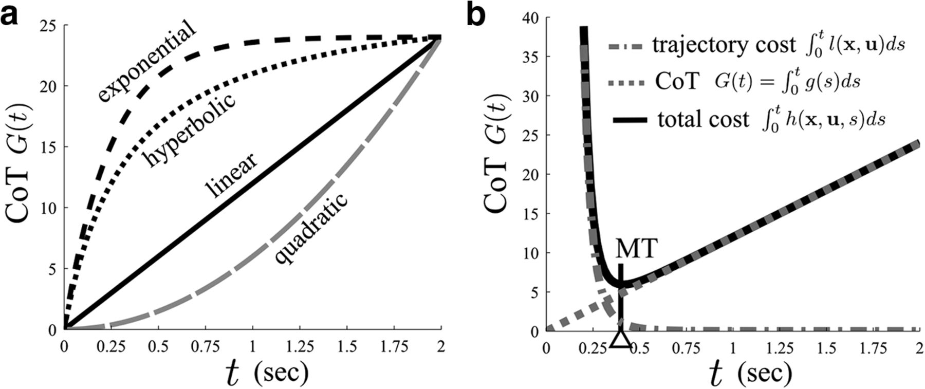
- Figure 1.
Illustration of the CoT theory. a, Previously proposed shapes of the CoT. Linear: G(t) = α t (Hoff, 1994; Liu and Todorov, 2007); hyperbolic: G(t) = α(1−1/(1+βt)) (Shadmehr, 2010; Shadmehr et al., 2010; Shadmehr and Mussa-Ivaldi, 2012); exponential: G(t) = α(1 − exp(− βt)) (Rigoux and Guigon, 2012); quadratic: G(t) = αt2 (Shadmehr et al., 2010). b, The CoT
 (assumed to be linear here for simplicity) sums with the trajectory cost , yielding a total cost that exhibits a “U” shape, the minimum being the optimal MT. It is noteworthy that, without the CoT, infinitely slow movements would be optimal for similar trajectory costs (which includes most of the costs proposed in the literature).
 - Figure 2.
Flowchart of the methodology. First, a model of the plant dynamics f and a trajectory cost l replicating the experimental trajectories with known MT must be available (gray boxes). From these experimental trajectories, the initial and final states of the system can be estimated (x0 and xf), as well as the movement duration t (black box). Finally, the corresponding optimal control (OC) problem in fixed-time t must be resolved (central ellipse) to evaluate the (constant) Hamiltonian ℋ0 along the optimal trajectory; this precisely yields the value of the infinitesimal CoT at time t. The partial time derivative of the value function could be used if preferred.
- Figure 3.
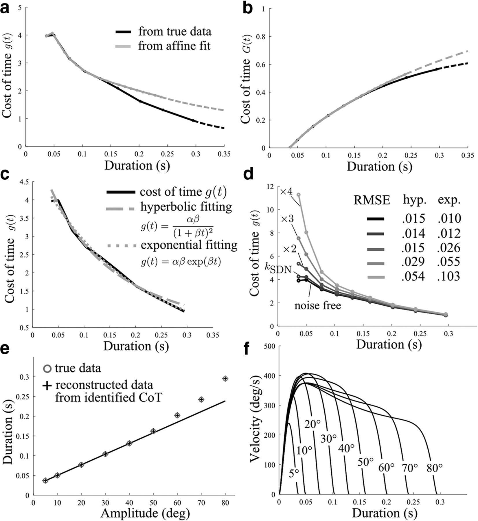
Cost of time underlying saccades, as inferred from data reported by Collewijn et al. (1988). a, Infinitesimal CoT g(t). To infer this cost, we used either the linear regression or the true data points exhibiting a growth larger than linear for amplitudes >40 degrees (see Collewijn et al., 1988). Dotted traces represent extrapolated parts of the CoT. Solid lines indicate values inferred using our inverse methodology. Our approach does not require fitting parameters or hypothesizing the shape of the time cost. b, Integral CoT G(t). The concavity of the CoT is obvious; and in particular, linear/convex costs can be ruled out (Shadmehr et al., 2010). c, Fitting of the infinitesimal CoT. We fitted g on the actual range of durations of observed saccades (i.e., from 36.5 to 295 ms). We considered both exponential and hyperbolic candidate functions. Best fitting parameters were as follows: (α, β) = (1.3, 4.3) and (α, β) = (0.9, 5.5) for the hyperbolic and exponential fits, respectively. d, Simulations in the stochastic case with different levels of signal-dependent noise (from kSDN to nkSDN with n = 2, 3, and 4, denoted by × n in the figure). RMSE is reported for hyperbolic (hyp.) and exponential (exp.) functions, respectively. With larger multiplicative noise, the CoT gets closer to the hyperbolic class of CoT. e, Verification of the amplitude–duration relationship as obtained from free time optimal control simulations with the CoT depicted in b (black trace). White-filled circles represent true data points (i.e., target values for the model). Black crosses represent simulated data (i.e., reconstructed values from the model). Both series of points matched perfectly because the methodology provides an exact solution to the problem of identifying the CoT associated with the observed amplitude–duration relationship. f, Velocity profiles of saccades of different amplitudes as predicted by the optimal control model.
- Figure 4.
Experimental amplitude–duration relationships for four different subjects (P1–P4) during arm reaching. Each dot indicates a single movement (trial) of amplitude lying between 5° and 95°. The result of a linear regression applied to the data is reported, namely, an affine fit of the form t = α a + β, with t being the MT in seconds and a the motion amplitude in degrees. Overall, even though intertrial variability was noticeable, a clear and significant (p < 0.001) affine trend was observed in all cases, as revealed by the relatively large R2 values.
- Figure 5.
Cost of time underlying single-joint arm reaching, as inferred from data reported in Figure 4. a, Infinitesimal CoT, g(t), for each of the four participants (P1–P4). Solid black traces represent values of g(t) inferred from linear regressions. Experimentally, MTs belonged to a certain interval [tmin, tmax] (emphasized by black filled circles), but it was possible to identify g(t) on a larger time interval by using predictions from the regression equation (black solid line). Dotted lines indicate extrapolated values of g(t) (i.e., values of g(t) not computed via our methodology). Light gray dots indicate values of g(t) inferred from single trials: each gray dot corresponds to a dot displayed in Figure 4. b, Integrated CoT, G(t). These curves were obtained by trapezoidal integration of the infinitesimal CoTs for each participant separately. The cost G(t) is only identified up to a constant, but in all cases the CoT exhibited a sigmoid-like shape on the range of actual motion durations (∼500–1500 ms on the present data).
- Figure 6.
Verification of the methodology via free time OC simulations. a, Amplitude–duration relationship recovered for participant P1 using the CoT identified in Figure 5b (black trace). Because the methodology is exact, the same regression equation as in Figure 4 is obtained. MT was left free and emerged automatically for each amplitude in these simulations. b, Associated movement kinematics. Velocity profiles remained bell-shaped in accordance with experimental observations and scaled with MT.
- Figure 7.
CoT consistency with respect to data fitting. a, Amplitude–duration relationship of two participants (left and right panels, respectively) who were asked to perform fully extended arm movements in the horizontal plane, for amplitudes ranging from 1° to 95°. In addition to linear functions, concave ones were tested for regression analysis (gray traces). The first log-based fitting had a zero-intercept constraint and was of the form t = αlog2(βa + 1) + γa (dark gray). The second log-based fitting (light gray) was chosen in the spirit of Fitts (1954) and the same as Young et al. (2009): that is, of the form t = αlog2(a/w + 1) + βa + γ where w denotes the actual width of the target (0.3 cm, i.e., ∼0.2 deg here). b, On the range of empirical times (∼300–1500 ms in these data), the CoT systematically exhibited a sigmoidal shape (filled circles on the traces). For smaller and larger times, we had to rely on extrapolations because data were no longer available (solid and dotted lines). Gray dots indicate values of g(t) identified on a single-trial basis and yield more noisy estimates.
- Figure 8.
Cost of time consistency (for participant P1, with the affine fit of the amplitude–duration relationship of Fig. 4). a, CoT when assuming various trajectory costs. Black represents the CoT for the torque change model, here scaled by a 0.05 factor for visualization purpose (infinitesimal CoT on left; integrated CoT on right). Grayscale represents the CoT identified from various trajectory costs (jerk, acceleration, absolute work, and torque). Although the specific values of the CoT necessarily changed with respect to the trajectory cost, its sigmoidal shape was nevertheless very robust. b, CoT when considering signal-dependent noise (kSDN) and a stochastic OC formulation. Increasing multiplicative noise essentially induced an increase of the CoT, but, again, the shape of the CoT remained sigmoidal. c, CoT when modeling muscle dynamics as second-order low-pass filters with different time constants and optimizing a neural effort cost. When still optimizing the torque change, no effects of the muscle dynamics were observed (result not depicted). When optimizing effort, the exact shape of the CoT depended on the underlying muscle dynamics. However, the shape of the infinitesimal CoT still showed a stiff increase after some time until a peak and followed by a slower decrease toward zero. Hence, the systematic nonmonotonicity of g(t) proves that the CoT is neither concave nor convex but possesses a generalized logistic shape. Notably, this conclusion can be drawn from the truly identified part of the curves, which is depicted via solid lines with filled markers. Dotted lines still indicate extrapolated values of the CoT outside of the range of actual measurements (using exponential functions here).
- Figure 9.
Cost of time underlying multijoint reaching, as inferred from data reported previously (van Beers et al., 2004; Young et al., 2009). a, Illustration of the task and optimal trajectories as predicted by the model. b, Affine amplitude–duration relationships reported by Young et al. (2009) for natural and quick speeds. c, Infinitesimal CoT g(t) identified for natural speed for rightward (dark gray) and leftward movements starting from different initial positions (black and light gray). d, Infinitesimal CoT identified for quick speed for the central starting position (light gray). Black dots indicate pointwise evaluations of g(t) when considering the center-out reaching task (e) and the corresponding MTs reported by van Beers et al. (2004). e, Center-out reaching task with the hand mobility ellipse depicted. f, MTs predicted by the model when solving free time OC problems using the previously identified CoT (i.e., c, d, light gray traces).


