

Abstract
Understanding visual perceptual learning (VPL) has become increasingly more challenging as new phenomena are discovered with novel stimuli and training paradigms. Although existing models aid our knowledge of critical aspects of VPL, the connections shown by these models between behavioral learning and plasticity across different brain areas are typically superficial. Most models explain VPL as readout from simple perceptual representations to decision areas and are not easily adaptable to explain new findings. Here, we show that a well -known instance of deep neural network (DNN), whereas not designed specifically for VPL, provides a computational model of VPL with enough complexity to be studied at many levels of analyses. After learning a Gabor orientation discrimination task, the DNN model reproduced key behavioral results, including increasing specificity with higher task precision, and also suggested that learning precise discriminations could transfer asymmetrically to coarse discriminations when the stimulus conditions varied. Consistent with the behavioral findings, the distribution of plasticity moved toward lower layers when task precision increased and this distribution was also modulated by tasks with different stimulus types. Furthermore, learning in the network units demonstrated close resemblance to extant electrophysiological recordings in monkey visual areas. Altogether, the DNN fulfilled predictions of existing theories regarding specificity and plasticity and reproduced findings of tuning changes in neurons of the primate visual areas. Although the comparisons were mostly qualitative, the DNN provides a new method of studying VPL, can serve as a test bed for theories, and assists in generating predictions for physiological investigations.
SIGNIFICANCE STATEMENT Visual perceptual learning (VPL) has been found to cause changes at multiple stages of the visual hierarchy. We found that training a deep neural network (DNN) on an orientation discrimination task produced behavioral and physiological patterns similar to those found in human and monkey experiments. Unlike existing VPL models, the DNN was pre-trained on natural images to reach high performance in object recognition, but was not designed specifically for VPL; however, it fulfilled predictions of existing theories regarding specificity and plasticity and reproduced findings of tuning changes in neurons of the primate visual areas. When used with care, this unbiased and deep-hierarchical model can provide new ways of studying VPL from behavior to physiology.
Introduction
Visual perceptual learning (VPL) refers to changes in sensitivity to visual stimuli through training or experience and has been demonstrated in the discrimination of simple features such as orientation, contrast, and dot motion direction, as well as more complicated patterns (Fiorentini and Berardi, 1980; Ball and Sekuler, 1982; Karni and Sagi, 1991; Ahissar and Hochstein, 1997; Mastropasqua et al., 2015). A common characteristic of VPL is its lack of transfer to untrained stimulus conditions, such as when rotated by 90° (Fiorentini and Berardi, 1981; Schoups et al., 1995; Crist et al., 1997). Due to their retinotopic mapping and orientation tuning (Hubel and Wiesel, 1968; Blasdel, 1992; Tootell et al., 1998), early visual areas have been hypothesized to contribute to VPL and its specificity (Fahle, 2004). Despite numerous examples supporting this hypothesis (Schoups et al., 2001; Bejjanki et al., 2011; Sagi, 2011; Jehee et al., 2012; Yu et al., 2016), there is substantial evidence that specificity does not require low-level changes (Dosher and Lu, 2017; Ghose et al., 2002) and there is great controversy regarding where learning happens in the visual hierarchy (Wang et al., 2016; Maniglia and Seitz, 2018).
Most models of VPL are artificial neural networks with user-parametrized receptive fields and shallow network structures. Trained using Hebbian-like learning rules (Sotiropoulos et al., 2011; Herzog et al., 2012; Dosher et al., 2013) or optimal decoding methods (Zhaoping et al., 2003), these models can reproduce and predict behavior, but rarely account for physiological data. Moreover, a key limitation of these models is that they do not address how the multiple known visual areas may contribute jointly to learning (Hung and Seitz, 2014). Other more conceptual models, such as the reverse hierarchy theory (RHT) (Ahissar and Hochstein, 1997, 2004) and the dual plasticity model (Watanabe and Sasaki, 2015), make predictions regarding what types of learning scenarios may lead to differential plasticity across visual areas, but these descriptive models do not predict specific changes in tuning properties of neurons. Therefore, there is a substantial need for a hierarchical model that can simulate learning and simultaneously produce behavioral and neurological outcomes.
A novel approach to modeling VPL can be found in deep neural networks (DNNs) which is readily adapted to learn different tasks. These DNNs have shown impressive correspondences to human behaviors and neural data from early visual areas and inferior temporal cortex (IT) (Khaligh-Razavi and Kriegeskorte, 2014; Yamins et al., 2014; Guclu and van Gerven, 2015; Cichy et al., 2016; Kheradpisheh et al., 2016; Eickenberg et al., 2017). This hierarchical system opens up new opportunities for VPL research (Kriegeskorte, 2015). As a start, Lee and Saxe (2014) and Saxe (2015) produced experimental and theoretical analyses that resembled RHT predictions using simple neural network architectures. Cohen and Weinshall (2017) used a shallow network to replicate relative performances of different training conditions for a wide range of behavioral data. To date, the extent to which DNNs can appropriately model physiological data of VPL remains unexplored.
Here, we trained a DNN model modified from AlexNet (Krizhevsky et al., 2012) to perform Gabor orientation and face gender discriminations. The network reflected human behavioral characteristics such as the dependence of specificity on stimulus precision (Ahissar and Hochstein, 1997; Jeter et al., 2009). Furthermore, the distribution of plasticity moved toward lower layers when task precision increased, and this distribution was also modulated by tasks with different types of stimulus. Most impressively, for orientation discrimination, the network units changed in a similar way to neurons in primate visual cortex, which helped reconcile divergent physiological findings in the literature (Schoups et al., 2001; Ghose et al., 2002). These results suggest that DNNs can serve as a computational model for studying the relationship between behavioral learning and plasticity across the visual hierarchy during VPL and how patterns of learning vary as a function of training parameters (Maniglia and Seitz, 2018).
Materials and Methods
Model.
An AlexNet-based DNN was used to simulate VPL. We briefly describe the network architecture here and refer readers to the original study for more details (Krizhevsky et al., 2012). The original AlexNet consists of eight layers of artificial neurons (units) connected through feedforward weights. In the first five layers, each unit is connected locally to a small patch of retinotopically arranged units in the previous layer or the input image. These connections are replicated spatially so that the same set of features is extracted at all locations through weight sharing. The operation that combines local connection with weight sharing is known as convolution. Activations in the last convolutional layer are sent to three fully connected layers with the last layer corresponding to object labels in the original object classification task. Unit activations are normalized in the first two convolutional layers to mimic lateral inhibition.
To construct the DNN model, we took only the first five convolutional layers of AlexNet and discarded the three fully connected layers to reduce model complexity. An additional readout unit was added to fully connect with the units in the last layer, forming a scalar representation of the stimulus in layer 6. We removed the last three layers of AlexNet because they exhibited low representational similarity to early visual areas but high similarity to IT and thus may be more relevant to object classification (Khaligh-Razavi and Kriegeskorte, 2014; Guclu and van Gerven, 2015); in addition, we assumed that early visual areas play a more critical role for Gabor orientation discrimination. We kept all five convolutional layers because one of our objectives was to study how learning was distributed over a visual hierarchy with more levels than most VPL models which are usually limited to two to three levels. In addition, activations in these five layers have been suggested to correspond to neural activities in V1–4 following a similar ascending order (Guclu and van Gerven, 2015).
The resulting six-layer network was further modified to model decision making in the two-interval two-alternative forced choice (2I-2AFC) paradigm (Fig. 1A). In this paradigm, a reference stimulus is first shown before a second target stimulus and the subject has to judge whether the second stimulus is more clockwise or more counterclockwise compared with the reference. In our DNN model, each of the reference and target images is processed by the same six-layer network that yields a scalar readout in layer 6 and the decision is made based on the difference between the representations with some noise. More precisely, two identical streams of the six-layer network produce scalar representations for the reference and target images, denoted by hr and ht, respectively. The network outputs a clockwise decision with probability (or confidence) p by passing the difference Δh = ht − hr through the following logistic function:
 This construction assumes perfect memory about the two representations computed using the same model architecture and parameters, and each choice is made with some decision noise. An advantage of using this 2I-2AFC architecture is that, when tested under transfer conditions (such as a new reference orientation), the network can still compare the target with the reference by taking the difference between the representations, whereas if only one stream exists, then the model cannot know the new reference orientation. We note that although this training paradigm is suitable for this network and was thus kept consistent throughout the simulations, it is different from those used in the physiological studies (Schoups et al., 2001; Ghose et al., 2002; Yang and Maunsell, 2004; Raiguel et al., 2006) with which we compare our network in the Results section. Learning could also be influenced by details of those experiments beyond what is accounted for by the present simulations.

Model structure and stimulus examples. A, Model architecture and a pair of Gabor stimuli. The network consists of two identical processing streams producing scalar representations, one for the reference (hr) and the other for the target (ht), and the difference of the two is used to obtain a probability of the target being more clockwise p(CW) through the sigmoid function. Darker colors indicate higher layers. Layers 1–5 consists of multiple units arranged in retinotopic order (rectangles) and convolutional weights (triple triangles, not indicative of the actual filter sizes or counts) to their previous layers or image and layer 6 has a single unit (dark orange circles) fully connected to layer 5 units (single triangles). Weights at each layer are shared between the two streams so that the representations of the two images are generated by the same parameters. Feedback is provided at the last sigmoidal unit. The Gabor examples have the following parameters: reference orientation: 30°, target orientation: 20°, contrast: 50%, wavelength: 20 pixels, noise SD: 5. B, Face examples morphed from three males and three females. The reference (ref) is paired with either a more masculine (M) or more feminine (F) target image, both morphed from the same two originals (M5 and F5), with the reference being the halfway morph. The number following the label indicates dissimilarity with the reference.
Task and stimuli.
All stimuli in the two experiments below were centered on 8-bit 227 × 227-pixel images with gray background.
Experiment 1.
The network was trained to classify whether the target Gabor stimulus was tilted clockwise or counter-clockwise compared with the reference. We trained the network on all combinations of the following parameters: orientation of reference Gabor from 0° to 165° at steps of 15° (12 orientations); angle separation between reference and target (0.5°, 1.0°, 2.0°, 5.0°, and 10.0°); and spatial wavelength (10, 20, 30, and 40 pixels). To simulate the short period of stimulus presentation and sensory noise, we kept the contrast low and added to each image isotropic Gaussian noise with the following parameters: signal contrast (20%, 30%, 40%, to 50% of the dynamic range) and SD of the Gaussian additive noise (5, 10, 15). In addition, the SD of the Gabor Gaussian window was 50 pixels. Noise was generated at run time independently for each image. An example of a Gabor stimulus pair is shown in Figure 1A.
Experiment 2.
The network was trained on face gender discrimination and Gabor orientation discrimination. For the face task, the network was trained to classify whether the target face was more masculine or feminine (closer to the original male or female in warping distance) than the reference face. Stimuli were face images with gender labels from the Photoface Dataset (Zafeiriou et al., 2011). A total of 647 male images and 74 female images with minimal facial hair were selected manually from the dataset and were captured in the frontal pose with the blank stare emotion. The bias in subject gender was addressed by subsampling to form balanced training and testing sets. The facemorpher toolbox (https://pypi.python.org/pypi/facemorpher/1.0.1) was used to create a reference halfway between a male and a female image.
To manipulate task difficulty, target images were created that varied in dissimilarity to the reference image ranging from 1 (closest to the reference) to 5 (the original male or female image) by adjusting a warping (mixing) parameter in the facemorpher toolbox. The reference and target were morphed from the same pair of the original faces. The network was trained and tested using 12-fold cross-validation. Each fold consists of images morphed from 49 males and 49 females for training (2401 pairs) and 25 males and 25 females for testing (625 pairs) randomly sampled from the full dataset. Examples of face stimuli at the five dissimilarity levels are shown in Figure 1B.
The Gabor stimulus had a wavelength of 20 pixels and the SD of the Gaussian window was 50. The reference angle ranged in 12 values from 0° to 165° at steps of 15° and the target image deviated from the reference by 0.5°, 1.0°, 2.0°, 5.0°, or 10.0°. For both the face and Gabor tasks in this experiment, contrast was set to 50% and noise SD was set to 5.
Training procedure.
In both experiments, network weights were initialized such that the readout weights in layer 6 were zeros and weights in the other lower layers were copied from an AlexNet trained on object recognition (downloaded from http://dl.caffe.berkeleyvision.org/bvlc_alexnet.caffemodel). The learning algorithm was a stochastic gradient descent (SGD) whereby the weights were changed to minimize the discrepancy between network output and stimulus label as follows:

 where α (0.0001) and μ (0.9) are learning rate and momentum, respectively, which are held constant through training, θt is the network weights at iteration t, and vt is the corresponding weight change. l(θt, It, Lt) is the cross-entropy loss that depends on the network weights, input image batch It of size 20 pairs and the corresponding labels Lt. Gradients were obtained by backpropagation of the loss through layers (Rumelhart et al., 1986).
Under this learning rule, zero initialization in the readout weights prevents the weights in lower layers from changing in the first iteration because the weights in those layers cannot affect performance and thus have zero gradients. This initialization can be interpreted as receiving instruction by subjects because all stimulus representations in the lower layers are fixed while the network briefly learns the task on the highest decision layer. After the first iteration, the readout weights will not be optimal due to small learning rate, so weights in the lower layers will start to change. Under each stimulus condition, the network was trained for 1000 iterations of 20-image batches so that one iteration is analogous to a small training block for human subjects. Independent noise was generated to each image at each iteration. We outline the limitations of the model in the Discussion section.
Behavioral performance.
The network's behavioral performance was estimated as the classification confidence (Eq. 1) of the correct label averaged over test trials. For the Gabor task, we tested the network's performance on stimuli generated from the same parameters as in training (trained condition) and also tested on stimuli generated from different parameters (transfer conditions), including rotating the reference by 45 or 90°, halving or doubling the spatial frequencies, and changing angle separations (or inverse precision) between the reference and target. A total of 200 pairs of Gabor stimuli were used in each test condition. For the face task, performance was tested on 625 unseen validation images. Performance was measured at 20 approximately logarithmically spaced iterations from 1 to 1000.
In Experiment 2, the contribution of DNN layers to performance was estimated using an accuracy drop measure defined as follows. Under each stimulus condition, we recorded the iteration at which the fully plastic network reached 95% accuracy, denoted by t95; we then trained a new network again from the original AlexNet weights under the same stimulus condition while freezing successively more layers from layer 1 and used the accuracy drop at t95 compared with the all plastic network as the contribution of the frozen layers. For example, suppose that the fully plastic network reached 95% accuracy at 100th iteration (t95 = 100) and, at this iteration, the network trained with frozen layer 1 had 90% accuracy and the network trained with the first two layers frozen had 85% accuracy. In this case, the first layer contributed 5% and the first two layers together contributed 10%. This accuracy drop does not indicate the contribution of each layer in isolation, but allows for different interactions within the plastic higher layers when varying the number of frozen lower layers.
Estimating learning in layers and neurons.
After training, weights at each layer were treated as a single vector and learning was measured based on the difference from pre-train values. Specifically, for a particular layer with N total connections to its lower layer, we denote the original N-dimensional weight vector trained on object classification as w (N and w are specified in AlexNet), the change in this vector after perceptual learning as δw, and define the layer change as follows:
 where i indexes each element in the weight vector. Under this measure, scaling the weight vector by a constant gives the same change regardless of dimensionality, reducing the effect of unequal weight dimensionalities on the magnitude of weight change. For the weights in the final readout layer that were initialized with zeros, the denominator in Equation 4 was set to N, effectively measuring the average change per connection in this layer. Due to the convolutional nature of the layers 1–5, drel1 is equal to the change in filters that are shared across location in those layers. When comparing weight change across layers, we focus on the first five layers unless otherwise stated. In addition, the following alternative layer change measures were also used:


 which produced different values, but they did not change the general effects of stimulus conditions on distribution of learning in weights. For the results in the main text, we report weight change in terms of drel1 unless otherwise stated. To measure learning of a single unit, we used the same equation but with w being the filter of each unit and N being the size of the filter.
Tuning curves.
For each unit in the network, we “recorded” its tuning curve before and after training by measuring its responses to Gabor stimuli presented at 100 orientations evenly spaced over the 180° cycle. The stimuli were a subset of those used in Experiment 1 which had noise SD 15, contrast 20%, and wavelength 10 pixels; this choice of wavelength means that one period of the sinusoidal component of the Gabor stimulus was contained within the receptive field of a layer 1 unit. The mean and SD at each test orientation were obtained by presenting the network with 50 realizations of noisy stimuli, followed by smoothing with a Gaussian kernel. The gradients of tuning curves were computed by filtering the mean response with a Laplace filter. Both the Gaussian and Laplace filters had an SD of 1°. The raw tuning curves were padded circularly to avoid boundary effect. Because the receptive fields were shared across locations, we only chose the units with receptive fields at the center of the image; therefore, the number of units measured at each layer equals the number of filter types (channels) in that layer. In addition, to ensure that units were properly driven by the stimulus, we excluded units that had mean activation over all orientations <1.0. The same procedure was repeated under the five precisions and 12 reference orientations as in Experiment 1 before and after training. No curve fitting was used. On average, training produced the following number of units for analyses: 79.4 of 96 in layer 1, 91.0 of 256 in layer 2, 237.3 of 384 in layer 3, 100.3 of 384 in layer 4, and 16.0 of 256 in layer 5. These numbers were approximately the same for the naive populations. Units were pooled together for analyses from training on the 12 reference orientations.
To compare with electrophysiological data in the literature, we measured the following attributes from tuning curves nonparametrically. The preferred orientation was determined by the orientation at which a unit attained its peak response. Tuning amplitude was taken to be the difference between the highest and lowest responses over orientation. Following Raiguel et al. (2006), the selectivity index (SI), a measure of tuning sharpness, was measured as follows:
 where si is the mean activation of a unit to a Gabor stimulus presented at orientation αi (index i ranges from 1 to 100). The normalized variance (or Fano factor, variance ratio) of the response at a particular orientation was taken as the ratio of response variance to the mean. Following Yang and Maunsell (2004), we measured the best discriminability of a unit by taking the minimum, over orientation, of response variance divided by tuning curve gradient squared.
To measure how much information about orientation was contained in a layer per neuron, we computed the average linear Fisher information (FI) (Seriès et al., 2004; Kanitscheider et al., 2015) at a particular orientation as follows:
 where f′(α) is a vector of tuning curve gradients at orientation α for n units in that layer (those with receptive fields at the center of the image), and Σ(α) is the corresponding response covariance matrix. In addition, independently for each unit, we measured FI as its tuning curve gradient squared divided by response variance at the measured orientation. For FI calculation, units with activity <1.0 at the measured orientation were excluded to avoid very low response variance.
Experimental design and statistical analyses.
In Experiment 1, the network was trained on Gabor orientation discrimination under 2880 conditions (12 reference orientation, four contrasts, four wavelengths, three noise levels, and five angular separations). In Experiment 2, the network was trained on 360 conditions in each of the Gabor and face tasks (12 reference orientations or training-testing data splits, five dissimilarity levels and zero to five frozen layers).
We performed our analyses on three levels. On the behavioral level, the effects of training and test angle separation on performance were tested using linear regression. On the layer level, the effects of layer number and training angle separation on layer change were also tested using linear regression. To determine whether the distribution of learning differed between tasks, we used two-way ANOVA to test whether there was an effect of task on layer change. At the unit level, we tested for significant changes in various tuning curve attributes recorded in the literature, using Kolmogorov–Smirnov (K–S) for distributional changes, Mann–Whitney U for changes in tuning curve attributes from training, and two-way ANOVA when neurons were grouped according to naive/trained and their preferred orientations. Finally, to test whether there was a relationship between the network's initial sensitivity to the trained orientation, we used a regression model described with the results. The significance level for all tests was 0.01. Bonferroni corrections were applied for multiple comparisons.
All code was written in Python with Caffe (http://caffe.berkeleyvision.org) for DNN stimulations and statsmodel (Seabold and Perktold, 2010) was used for statistical analyses. Code and stimulated data are available on request.
Results
Behavior
The network was trained to discriminate whether the target Gabor patch was more clockwise or more counterclockwise to the reference, repeated in 2880 conditions (12 reference orientation, four contrasts, four wavelengths, three noise levels, and five precisions or angle separations). The performance trajectories grouped by precision are shown in Figure 2A (top, for the first 50 iterations, see Fig. 2-1) for the trained and transfer conditions of rotated reference orientations (clockwise by 45 or 90°) and scaled spatial frequencies (halved or doubled). The accuracy measured at the first iteration (analogous to naive real subjects) indicates the initial performance when only the readout layer changed. Both initial performance and learning rate under the trained condition were superior for the less precise tasks, consistent with findings from the human literature (Ahissar and Hochstein, 1997; Jeter et al., 2009). Percentage correct increased in a similar way to human data on Vernier discrimination (Herzog and Fahlet, 1997) and motion direction discrimination (Liu and Weinshall, 2000). Convergence of performance for the transfer stimuli required more training (note the logarithmic x-axis in Fig. 2A) than for the trained stimuli, which may imply that much more training examples are necessary to achieve mastery on the transfer stimuli, consistent with some studies of tactile perceptual learning (Dempsey-Jones et al., 2016).

Performance of the model when trained under various angle separations and tested at the trained and transfer conditions: reference orientation rotated clockwise by 45 (ori + 45) or 90° (ori + 90) and spatial frequency halved (SF × 0.5) or doubled (SF × 2.0). For statistical details, see Table 2-1. A, Accuracy (top) and transfer index (bottom) trajectories against training iterations. Darker blue indicates finer precision. 1 SEM error bars are hardly visible. For accuracies plotted as mean ± SD during the first 50 iterations, see Figure 2-1. B, Final performance under the four transfer conditions. There was a significant positive main effect of log angle separation in each of the four transfer conditions (p < 0.0001, R2 > 0.2 in all conditions), indicating greater transfer for coarser precisions. Error bar indicates 1 SD. C, Final mean accuracies when the network was trained and tested on all combinations of training and test precisions. The diagonal lines in the four transfer conditions indicate equal training and test precision for which the accuracies are also shown in B. For each transfer condition, there was a strong positive main effect of log test separation (p < 0.0001, R2 > 0.35 in all conditions) shown as increasing color gradient from bottom to top; Log training separation also had a weaker but significant negative effect (p < 0.0001 in all conditions, R2 > 0.05 in all conditions except for angle + 90 where R2 = 0.018), shown as decreasing color gradient from left to right. Higher training precisions enhanced performance at transfer to low precisions, shown as higher accuracy on top-left quadrants compared with lower-right quadrants.
Table 2-1
Figure 2-1
Moreover, we characterized the dynamics of transfer by calculating the transfer index as the ratio of transfer accuracy to the corresponding trained accuracy. As shown in Figure 2A (bottom), this ratio decreased initially but started to rise slowly for all conditions, and the trajectory for orthogonal transfer (ori+90) under the highest precision was almost flat toward the end of training. Similar reduction in transfer index with increasing training sessions has been demonstrated in human experiments (Jeter et al., 2010).
Figure 2B shows the final transfer performance grouped by transfer conditions and training precision. All transfer accuracies were below 1.0, especially for the orientation transfers, indicating various degrees of learning specificity. A linear regression on transfer accuracy showed a significant positive main effect of log angle separation in all four transfer conditions (p < 0.0001; for details, see Table 2-1, implying better transfer performance for less precise training. This result is consistent with experimental data and theoretical prediction that greater specificity happens in finer precision tasks (Ahissar and Hochstein, 1997; Liu, 1999; Liu and Weinshall, 2000).
However, the transfer precisions were the same as used during the respective trained conditions and thus varied in intrinsic discriminability in the above comparisons, which could have determined the observed pattern on transfer conditions. We thus tested each trained network on all angle separations to determine whether we could reproduce human psychophysical data (Jeter et al., 2009) in which a difference in test precision affects transfer more than training precision. Indeed, Figure 2C shows a strong positive main effect of test separation (p < 0.001 and R2 > 0.35 for all transfer conditions); however, we also found that training separation had a significant effect (p < 0.001) in all transfer conditions and the effect size was the smallest in orthogonal orientation transfer (for details, see Table 2-1). The more substantial transfer to 45° from trained orientations compared with 90° could be due to a larger overlap between the trained and transfer orientation representations of the network units. Therefore, despite the observation of diminishing transfer with increasing precision when the training and test precisions are equal (diagonal lines in Fig. 2C), the analyses across all precision combinations predict that transfer is more pronounced from precise to coarse discrimination than vice versa, although transfer can be very small at the orthogonal orientation.
Overall, these behavioral findings are consistent with extant behavioral and modeling results of perceptual learning. Furthermore, the DNN model can simulate a wide number of trained conditions and makes predictions regarding the relative performances and learning rates of the trained stimuli compared with that of transfer stimuli. However, it is expected that some details of this DNN′s behavioral results will necessarily differ from experimental data.
Distribution of learning across layers
Learning in the weight space
We next examined the time course of learning across the layers as a function of precision calculated using Equation 4 and shown in Figure 3A. Overall, all layers changed faster at the beginning of training in coarse than in precise angle separations, training precise angle separations produced greater overall changes. While the highest readout layer (layer 6) changed faster than the other layers, which was also found by Saxe (2015) on a linear deep network, this was likely a consequence of zero initialization in the readout weights. This result suggests that, when performance is at chance level, due to naivety to the task, information about the stimulus label cannot be passed on to lower layers while the performance is close to chance. Due to this mismatch of weight initialization, we focus on layers 1–5 with weights initialized from the pre-trained AlexNet.

Layer change under different training precisions. A, Layer change (Eq. 4) trajectories during learning. Lighter colors indicate larger angle separations. 1 SEM error bars are hardly visible. B, Iteration at which the rate of change peaked (PSI). Excluding layer 6, there were significant negative main effects of log angle separation (β = −37.24, t(14397) = −100.02, p ≈ 0.0, R2 = 0.41) and layer number (β = −1.07, t(14397) = −8.73, p = 2.9 × 10⁻¹⁸, R2 = 0.0031) on PSI, suggesting that layer change started to asymptote earlier in higher layers and finer precisions. For individual precisions, layer number had a significant effect only for the two smallest angle separations (p < 0.0001; for details, see Table 3-1). C, Final layer change. Ignoring layer 6, for which the change was measured differently, a linear regression analysis on the logarithm of layer change yielded significant negative main effects of log angle separation (β = −1.0, t(14397) = −208.4, p ≈ 0.0, R2 = 0.66) and layer number (β = −0.15, t(14397) = −91.2, p ≈ 0.0, R2 = 0.13), implying greater layer change in lower layers and finer precisions. D, Ratio of final layer change relative to the change under the easiest condition (10.0°). Changes in lower layers increased by a larger factor than higher layers when precision was high. B–D, Error bar indicates 1 SEM.
Table 3-1
To characterize learning across layers, we studied when and how much each layer changed during training. To quantify when significant learning happened in each layer, we estimated the iteration at which the gradient of a trajectory reached its peak (peak speed iteration, PSI; shown in Figure 3B). In layers 1–5, we observed significant negative main effects of log angle separation (β = −46.02, t(14396) = −52.93, p ≈ 0.0, R2 = 0.40) and layer number (β = −2.07, t(14396) = −13.65, p = 3.6 × 10−42, R2 = 0.0031) and a positive interaction of the two (β = 2.93, t(14396) = 11.16, p = 8.0 × 10⁻²⁹, R2 = 0.0050) on PSI, suggesting that layer change started to asymptote later for lower layers and smaller angle separations. For individual precision conditions, a linear regression analysis showed a significant negative effect of layer number on PSI only in the two most precise tasks (p < 0.0001; for details, see Table 3-1). Therefore, under high precisions, the order of change across layers is consistent with the reverse hierarchy theory prediction that higher visual areas change before earlier ones (Ahissar and Hochstein, 1997).
The final layer change at the end of training is shown in Figure 3C. For a better visual comparison, we calculated the relative layer change under each stimulus condition by taking the ratio of layer change against the change that resulted from training at the same stimulus conditions but under the coarsest angle separation (Fig. 3D). Weight changes in lower layers increased by a factor larger than those in higher layers except layer 5. A linear regression analysis on the changes in layers 1–5 revealed significant negative main effects of log angle separation (β = −0.0060, t = −87.25, p ≈ 0.0, R2 = 0.34) and layer number (8.6 × −10−4, p ≈ 0.0, R2 = 0.092) and a positive interaction of the two (0.00010, t = 49.23, p ≈ 0.0, R2 = 0.082). The interaction of angle separation × layer number on layer change is consistent with the prediction that higher-precision training induces more change lower in the hierarchy (Ahissar and Hochstein, 1997).
Change of information about orientation
Although we have considered thus far the changes in the weights of the DNN, there is still a question of how the information about orientation changed across layers and how this may vary as a function of training precision. We address this by showing in Figure 4 the covariance-weighted linear Fisher information (FI) (Eq. 6) of the trained and naive unit population at each layer and each test orientation when trained at each angle separation. The tuning curves used to evaluate FI were obtained from the units with receptive fields at the center of the image (see Materials and Methods). A prominent observation is that FI increased most dramatically at the highest layers under the most precise task and diminished toward lower layers and coarser precisions. Lower layers saw significant FI improvement only in the most precise tasks, whereas higher layers increased FI in all precisions.

Linear FI defined in Equation 6 of the trained (black) and naive (gray) populations at each layer and each test orientation and when trained at each precision. Each line is drawn as mean and 1 SEM envelope. Only units with receptive fields at the center of the image and with minimum activation of 1.0 are included. Asterisk indicates significant increase in mean FI within 10° of the trained orientation (threshold p = 0.01, Mann–Whitney U, Bonferroni corrected for 5 layers × 5 angle separations). The FI values at layer 5 do not reflect real discrimination thresholds because the readout was noisy.
However, the quantitative trend of FI increase was contrary to the layer change where more substantial learning happened in the lower layers. Notably, despite the large change in layer 1 weights (Fig. 3C), there was no visible change in FI. The large FI increase in higher layers may not be surprising due to a single hierarchy with readout on the top layer and the accumulation of weight changes from the lower layers.
In addition, we observed patterns of FI over orientations. After training at the finest precision, the top layers exhibited significant and substantial increase of FI around the trained orientation; FI fell off at ~20° away from trained orientation but remained noticeable until the orthogonal orientation. This could account for the transfer behavior predicted by the network (Fig. 2) where learning transferred more substantially if the Gabor stimulus was rotated by 45° rather than the more common 90°.
These data show that the increase of information about orientation over network layer changes as a function of training precision. Later, we will discuss how this information in the pre-trained network may affect learning (see Fig. 10).
Effect of feature complexity on distribution of learning
Are the observed layer changes prescribed solely by the network structure and learning rule regardless of the task? To find out whether these patterns were task specific, we simulated learning of a “higher-level” face gender discrimination task and investigated its effect on the distribution of learning in network weights compared with Gabor orientation discrimination. In the face task, difficulty was manipulated by morphing between male and female face images and the network was trained to discriminate whether the target was more masculine or feminine compared with the reference. Both tasks were repeated under 360 conditions (12 reference orientations for the Gabor task or 12 training-testing data splits for the face task, five dissimilarity levels and zero to five frozen layers). By the end of training, the fully plastic network reached test accuracy above 95% for all stimulus conditions. In this section, we assume that learning in stimulus representation happened in the lower 5 layers and do not analyze the changes in layer 6.
Due to the hierarchical representation from earlier to later visual areas, one may hypothesize that learning in lower layers of the DNN would play a more important role in performance for the Gabor task relative to the face task. To quantify the contributions of layers on performance, we measured how much accuracy dropped when more lower layers were frozen (keeping weights fixed) at a particular iteration during training (see Methods and Materials). Results are shown in Figure 5A. Performance in the Gabor task dropped considerably when freezing layer 2 onward, whereas, in the face task, learning was significantly impaired only when freezing all the first four layers or more. Although this freezing technique is unnatural and it is possible that compensatory changes occurred that did not reflect properties of learning in the fully plastic network, these results support the hypothesis that the higher layers are more informative for judgements on more complex stimulus and the earlier layers are so for more precise and simpler ones.

Effect of different tasks (Gabor orientation and face gender discriminations) on performance and layer change. A, Accuracy drop as successive low layers were frozen at the iteration where the fully plastic network reached 95% accuracy for the two tasks. Asterisk indicates significant drop from zero (threshold p = 0.01, 1-sample t test against zero, Bonferroni-corrected for 5 frozen layers × 5 dissimilarities). Performance was impaired when freezing layer 2 onward in the Gabor task and when freezing layer 4 onward in the face task. The largest incremental performance drop happened in layer 3 for the Gabor task and layer 5 for the face task. B, Distribution of learning over layers when the network was trained on the two tasks if the network was fully plastic (left) or if layer 1 was frozen (right). There was a significant interaction of layer × task on layer change proportion (p < 0.0001, 2-way ANOVA; for details, see Table 5-1). For demonstration of robustness to other measures of layer change, see Figure 5-1. Asterisk indicates significant difference in the layer change proportion between the two tasks (threshold p = 0.01, Mann–Whitney U, Bonferroni corrected for 5 or 4 layers). Error bar indicates 1 SEM.
Table 5-1
Figure 5-1
To further test whether the distribution of learning depended on task, we calculated the proportions of layer change in the first five layers by normalizing these changes against their sum (Fig. 5B; for other layer change measures, see Fig. 5-1). Because the first layer did not have a large contribution to performance (Fig. 5A) and response normalization happened after the first layer, we also compared the layer change proportions after training while freezing the weights in layer 1 at pre-trained values. A two-way ANOVA revealed a significant interaction of layer × task on layer change proportion in both network conditions (p < 0.0001; for details, see Table 5-1), suggesting that task indeed changed the distribution of learning over layers. Post hoc analysis showed a significant increase in weight change proportions in layers 4 and 5 and a significant decrease in layer 2 (Mann–Whitney U, threshold p = 0.01, Bonferroni-corrected for 5 or 4 layers). Therefore, more weight change happened in lower layers when learning the “low-level” Gabor task, and higher layers acquired more change in the “high-level” face task, consistent with theories of VPL (Ahissar and Hochstein, 1997, 2004; Watanabe and Sasaki, 2015).
One should be careful when interpreting values of layer change defined by Equation 4. For instance, the layer with maximum change varied between layers 1 and 3 depending on how these changes were calculated (e.g. Eqs. 4a–4c), although the general effects of precision and task on layer change were consistent under other weight change measures (Fig. 5-1). In addition, it may be tempting to infer the relationship between layer contribution and change; however, freezing early layers created different interactions between the higher plastic layers, which makes it difficult to compare directly layer contribution with the layer change obtained by the fully plastic network.
Therefore, by analyzing the weight changes in the network layers, we have shown that the distribution of learning over the network hierarchy moves toward lower layers for more precise discriminations of simple features and toward higher layers for less precise or more complex stimuli such as faces. To determine to what extent this DNN model can reflect changes in the brain during perceptual learning, we compared activations of individual units in the network with activities of real neurons in the brain recorded by electrophysiology, as described in the following section.
Tuning changes of single units
Single units in different layers of the DNN model were examined to determine whether the changes in these units were similar to those in monkey neurons after VPL. A key target of this investigation was to address computationally some of the significant findings in the literature that had led to diverging interpretations of plasticity within the visual hierarchy. Previous research on DNNs found that the representational geometries of layers 2 and 3 (but not layer 1) in this network were analogous to those in human V1–3 (Khaligh-Razavi and Kriegeskorte, 2014), so we focused our analyses on layers 2–5.
We compared the network units with V1–2 and V4 neurons recorded in four electrophysiological studies; animals in these studies were trained to discriminate orientations of Gabor patches. Schoups et al. (2001) discovered an increase in the tuning curve slope at the trained orientation for units tuned to 12–20° away from trained orientation. The same group (Raiguel et al., 2006) later found in V4 a similar change, along with other effects of training. These studies used a single-interval 2AFC training paradigm with an implicit reference that was never shown. Conversely, Ghose et al. (2002) used a 2I-2AFC training paradigm in which an irrelevant feature of the stimulus (spatial frequency) varied between two values through training. Contrary to Schoups et al. (2001), they did not find significant changes in V1–2 regarding orientation tuning (except one case), but the final discrimination thresholds reached by the subjects were higher. This group later revealed several changes in V4 using the same training paradigm (Yang and Maunsell, 2004). We hypothesized that the differences between these studies could be explained by differences in stimulus precision during training. To test this, we trained the network on a common task, the 2I-2AFC Gabor discrimination paradigm, and tested whether changing training precision, holding everything else constant, was sufficient to reconcile the gross differences observed between these studies.
Overall, it appears that V1–2 only changed when the discrimination threshold was small (0.5–1.2° by Schoups et al., 2001, smaller than 3.3–7.3° by Ghose et al., 2002) and V4 changed in both studies though the discrimination thresholds were similar to each other (1.9–3.0° by Raiguel et al., 2006 and 1.9–5.4° by Yang and Maunsell, 2004). Given the pattern of change in layer FI demonstrated earlier (Fig. 4), we hypothesized that: (1) the contradictory results in V1–2 (corresponding to lower layers in the network) were due to the mismatch of the final thresholds reached by the subjects in the two V1–2 studies, and (2) the change in V4 (corresponding to higher layers in the network) should persist from fine to coarse precisions in which V1–2 did not change.
To test the first hypothesis using the DNN model, we approximately matched the angle separations used to train the network with the discrimination thresholds reached by the monkeys, 1.0° for high and 5.0° for low precisions, and compared network units in layer 2 with real V1–2 neurons. We then compared the tuning attributes of units in layer 5 with those of V4 neurons to test our second hypothesis. These choices were mainly motivated by previous research on comparing this particular network with the visual brain areas (Khaligh-Razavi and Kriegeskorte, 2014; Guclu and van Gerven, 2015; Eickenberg et al., 2017). It should be noted that we used the same spatial frequency for the reference and target (more similar to Schoups et al. (2001) than to Ghose et al. (2002)); therefore, whereas we found that modeling the differences in thresholds is sufficient to account for many differences in physiological findings between the four studies, it is likely that other task and stimulus differences also contributed to the different profiles of learning.
Tuning curves were obtained from the units with receptive fields at the center of the image and are shown in Figure 6A for layers 2 and 5. Many of the layer 2 units showed bell-shaped tuning curves with clear orientation preferences, mirroring the reported similarity between these two layers with human early visual areas. In addition, there were also intriguing tuning curves that showed more than one tuning peaks, which may not be physiologically plausible. Tuning curves in layer 5 were harder to interpret, with some units showing clear orientation tuning and the rest likely tuned to features other than Gabor patches.
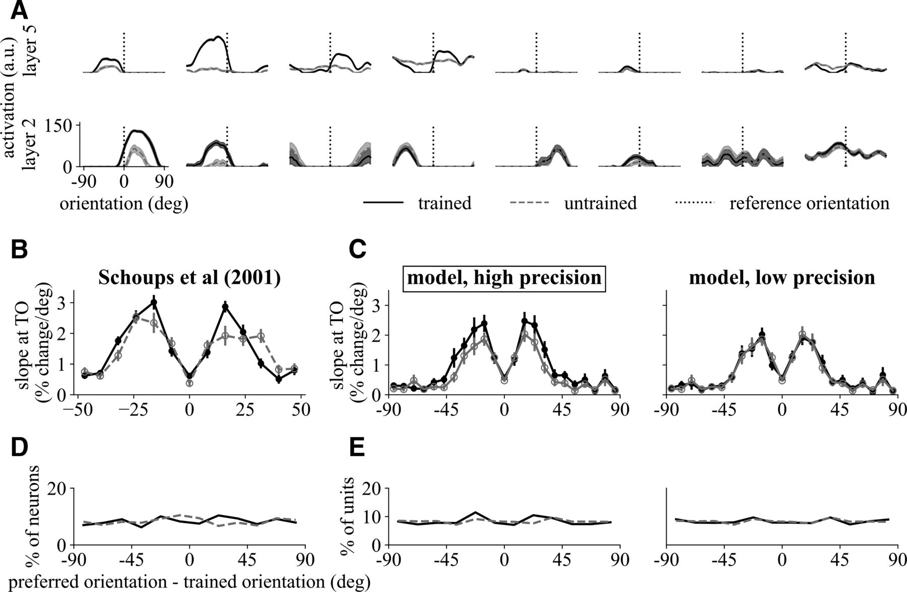
A, Tuning curve examples of network units before (gray dashed) and after (black solid) training in layers 2 and 5. B–E, Comparison between V1 neurons trained under high precision in Schoups et al. (2001) with model units in layer 2 trained under high (1.0°, matching with experiment) and low (5.0°) precisions. B, Slope of normalized tuning curve at trained orientation for trained and naive V1 neurons grouped according to preferred orientation. C, Same as B but from model units. Units tuned around 20° increased their slope (after normalization) magnitude at trained orientation only under high precision. For statistical test details, see Table 6-1; for layer 3 and other precisions, see Figure 6-1. D, Distribution of preferred orientation in V1 was approximately uniform before and after training. E, Same as D but from model units. There was no significant difference in the distribution of preferred orientation between the trained and naive populations under either of the two precisions (p > 0.9, K–S; for details, see Table 6-2; for layer 3 and other precisions, see Figure 6-2). B and D were adapted with permission from Schoups et al. (2001).
Table 6-1
Figure 6-1
Table 6-2
Figure 6-2
Lower layers trained under high precision (Schoups et al., 2001)
We first investigated whether this DNN model could reproduce findings on V1 neurons by Schoups et al. (2001), who found that monkeys obtained very small thresholds (~1°) and V1 neurons showed a change in the slope of tuning curve at trained orientation for neurons tuned between 12° and 20° from trained orientation (Fig. 6B, for statistical details, see Table 6-1; for layer 3 and other precisions, see Fig. 6-1). Similar to their procedure, we took the orientation of the maximum response of a unit as its preferred orientation and grouped all units by preferred orientation relative to trained orientation. The slope of the tuning curve at trained orientation was evaluated after normalization by maximum activation (as done for neural data in Schoups et al., 2001). The results for layer 2 units (Fig. 6C) showed a similar slope increase for units tuned away from trained orientation, overlapping but broader than the range found in V1 neurons, when trained under high precision but not low precision.
Despite a change in tuning slope, Schoups et al. (2001) found that the preferred orientations of neurons were evenly distributed over all orientations before and after training (Fig. 6D). This was also the case for the network units which showed no significant difference between trained and naive distributions of preferred orientation in either of the precisions (Fig. 6E, p > 0.9, K–S; for details, see Table 6-2; for layer 3 and other precisions, see Fig. 6-2).
Overall, these data from lower-layer units demonstrated an impressive qualitative similarity to data from Schoups et al. (2001) when the network was trained on high precision. We next look at tuning curve changes in low precision training.
Lower areas trained under low precision (Ghose et al., 2002)
Contrary to Schoups et al. (2001), Ghose et al. (2002) found very little change in V1–2 neurons after training. The tuning amplitude of V1 and V2 neurons tuned around the trained orientation did not differ significantly from other neurons after training (Fig. 7A). However, the monkeys trained by Ghose et al. (2002) achieved relatively poorer discrimination thresholds (~5°) and, when we modeled this as low precision training, we also found no significant effect of preferred orientation on tuning amplitude in layers 2–3 (Fig. 7B, p = 0.30, Mann–Whitney U; for details, see Table 7-1; for layer 3 and other precisions, see Fig. 7-1). In addition, Ghose et al. (2002) found no significant change in the variance ratio for V1–2 neurons (Fig. 7C), which was replicated by our network units at both precisions (Fig. 7D, p > 0.6, Mann–Whitney U; for details, see Table 7-2; for layer 3 and other precisions, see Fig. 7-2). Ghose et al. (2002) did observe a decrease in the number of neurons tuned to the trained orientation in V1, but not in V2 (data not shown), contrary to Schoups et al. (2001). In our model, no such change was found in either high or low precision (Fig. 6D); therefore, here, the model did not agree with the data.

Comparison between V1–2 neurons trained under low precision in Ghose et al. (2002) with model units in layers 2 and 3 trained under high (1.0°) and low (5.0°, matching with experiment) precisions. Black bar indicates the orientation bin that contains the trained orientation. A, No significant effect of preferred orientation was found on tuning amplitude. B, Same as A but from model units. Preferred orientation had a significant effect only in layer 3 when trained under high precision (p < 0.0001, one-way ANOVA; for details, see Table 7-1; for layer 3 and other precisions, see Figure 7-1). C, No significant effect of preferred orientation was found on variance ratio. D, Same as C but from model units. No significant effect of preferred orientation was found on variance ratio (p > 0.6, one-way ANOVA; for details, see Table 7-2; for layer 3 and other precisions, see Figure 7-2). A and C were adapted with permission from Ghose et al. (2002).
Table 7-1
Figure 7-1
Table 7-2
Figure 7-2
Therefore, under low precision, we did not find significant changes in tuning attributes in lower layers, which was also the case for Ghose et al. (2002) except for the preferred orientation distribution in V1. Together with the comparisons under high training precision in previous sections, our first hypothesis was supported by our simulations. The key in replicating these data is the observation that the precision of training has a profound effect on the distribution of learning across layers. By accounting for the different orientation thresholds found across studies and laboratories, the DNN model can address well the different observations, which was also demonstrated in a simpler network (Saxe, 2015). In addition, the partial specificity of the network trained under low precisions (Fig. 2B) did not require orientation-specific changes in lower layers, consistent with previous models and data (Petrov et al., 2005; Sotiropoulos et al., 2011; Dosher et al., 2013).
Higher layers compared with data of Raiguel et al. (2006)
Although neurons in primary visual cortex showed plasticity that was largely limited to high-precision conditions, neurons in V4 generally showed more susceptibility to VPL (Yang and Maunsell, 2004; Raiguel et al., 2006). We hypothesized that changes in V4 neurons should happen in both low and high precisions and tested this hypothesis by comparing the tuning attributes of units in layer 5 (layer 4 in Extended Data) with recordings in those studies.
We first compared the network units with the results of Raiguel et al. (2006) showing that, similar to V1 (Fig. 6B), V4 neurons tuned 22–67° away from trained orientation significantly increased their slopes at trained orientation (Fig. 8A). This effect was replicated in the model units (Fig. 8B), which, unlike layer 2 (Fig. 6C), showed significant increase in tuning slope not only in high but also in low precisions (p < 0.0002, two-way ANOVA; for details, see Table 8-1; for layer 4 and other precisions, see Fig. 8-1), although these units with increased slopes were tuned much closer to trained orientation than V4 neurons.

Comparison between V4 neurons in Raiguel et al. (2006) with model units in layer 5 trained under high (1.0°) and low (5.0°) precisions. Black and white bars indicate trained and naive populations, respectively. A, Neurons tuned 22–67° away from trained orientation increased their slopes at trained orientation. Asterisk indicates significant increase in slope before and after training. B, Same as A but from model units. There was a significant interaction of training × preferred orientation under either of the precisions (p < 0.0002, two-way ANOVA; for details, see Table 8-1; for layer 4 and other precisions, see Figure 8-1). Asterisk indicates significant increase in slope before and after training (threshold p = 0.01, Mann–Whitney U, Bonferroni corrected for six orientation bins). Only neurons tuned within 48° of trained orientation are shown; other neurons did not change significantly after training. C, Distribution of preferred orientation shifted away from uniform after training. D, Same as C but from model units. The units under both precisions altered their preferred orientation distribution, which became significantly different from a uniform distribution (p < 0.003, K–S; for details, see Table 8-2; for layer 4 and other precisions, see Figure 8-2). E–H, Black and gray dashed lines indicate trained and naive distribution means, respectively. E, SI of V4 neurons increased significantly after training. F, Same as E but from model units. Training produced a significant increase in SI under high precision (p < 0.0001, Mann–Whitney U; for details, see Table 8-3; for layer 4 and other precisions, see Figure 8-3). G, Training significantly reduced normalized variance of V4 neurons. H, Same as G but from model units. Normalized variance was significantly reduced after training under both precisions (p < 0.001, Mann–Whitney U; for details, see Table 8-4; for layer 4 and other precisions, see Figure 8-4). A, C, E, and G were adapted with permission from Raiguel et al. (2006).
Table 8-1
Figure 8-1
Table 8-2
Figure 8-2
Table 8-3
Figure 8-3
Table 8-4
Figure 8-4
Furthermore, in monkey V4, the distribution of preferred orientation became nonuniform after training (Fig. 8C). In our model, this distribution also became significantly different from a uniform distribution, as revealed by a K–S test in both conditions (p < 0.003, K–S; for details, see Table 8-2; for layer 4 and other precisions, see Fig. 8-2). This is in contrast to layer 2, which only showed such a change for high precision (Fig. 6E). There was also a substantial increase in the number of neurons tuned very close to trained orientation.
The strength of orientation tuning, measured by selectivity index (SI) defined in Equation 5, was found to increase in V4 after training (Fig. 8E). Similar results were found in the model (Fig. 8F) in which SI increased significantly when trained under high precision (p < 0.0001) but not under low precision (p = 0.10, Mann–Whitney U; for details, see Table 8-3; for layer 4 and other precisions, see Fig. 8-3). Although these results suggest that higher-layer units became sharper after training when the precision was high, the shape of this distribution in layers 4 and 5 did not match with real V4 neurons.
Raiguel et al. (2006) also discovered that training reduced response variability at the preferred orientation quantified by the normalized variance (Fig. 8G). We found the same in our model units (Fig. 8H) at both precisions (p < 0.001, Mann–Whitney U; for details, see Table 8-4; for layer 4 and other precisions, see Fig. 8-4), suggesting that noisy units in the lower layers might be rejected by higher layers (Dosher and Lu, 1998).
Higher layers compared with data of Yang and Maunsell (2004)
Finally, we addressed whether the network units also replicated the findings of Yang and Maunsell (2004) in which monkeys achieved a threshold comparable with (Raiguel et al., 2006). Overall, in contrast to the V1 study from the same group (Ghose et al., 2002), Yang and Maunsell (2004) found many tuning changes in V4. First, tuning amplitude of V4 neurons increased significantly after training (Fig. 9A) and the same was observed in the model under both precisions (p < 0.0001, Mann–Whitney U; for details, see Table 9-1; for layer 4 and other precisions, see Fig. 9-1). Second, V4 neurons significantly lower their best discriminability (Fig. 9C) after training, suggesting that finer orientation differences could be detected. Units in the model (Fig. 9C) reproduced the same change in both precision levels (p < 0.0005, Mann–Whitney U; for details, see Table 9-2; for layer 4 and other precisions, see Fig. 9-2).

Comparison between V4 neurons in Yang and Maunsell (2004) with model units in layer 5 trained under high (1.0°) and low (5.0°) precisions. A–D, Black and white bars indicate trained and naive populations, respectively; black and gray dashed lines indicate trained and naive distribution medians, respectively. A, Training significantly increased the tuning amplitude of V4 neurons. B, Same as A but from model units. Training significantly increased response amplitude for both precisions (p < 0.0001, Mann–Whitney U; for details, see Table 9-1; for layer 4 and other precisions, see Figure 9-1). C, Training produced a significant reduction in best discriminability (lower indicates better discriminability) for V4 neurons. D, Same as B but from model units. Training significantly reduced the best discriminability for both precisions (p < 0.0005, Mann–Whitney U; for details, see Table 9-2; for layer 4 and other precisions, see Figure 9-2). E, Training resulted in narrower normalized tuning curves (by maximum response). F, Same as E but from model units. Activation was significantly lower after training for the nonpreferred orientation range (>45° away of trained orientation) than preferred orientation range in high precision (p < 0.0001, two-way ANOVA; for details, see Table 9-3; for layer 4 and other precisions, see Figure 9-3). Red lines indicate orientations with significant reduction in activation (threshold p = 0.01, Mann–Whitney U, Bonferroni corrected for 100 test orientations). Curves are mean with 1 SEM envelope. A, C, E, and G were adapted with permission from Yang and Maunsell (2004).
Table 9-1
Figure 9-1
Table 9-2
Figure 9-2
Table 9-3
Figure 9-3
Yang and Maunsell (2004) went on to show that these changes were not simply a result of the scaling, but rather the narrowing, of tuning curves (Fig. 9E). In layer 5 of the model, the tuning widths of naive units were already smaller than trained V4 neurons; nonetheless, we found that, under high precision, the mean activation of layer-5 units (Fig. 9F) in the nonpreferred orientation range (45° away from preferred orientation) was significantly more reduced than that in the preferred orientation range (within 45° of preferred orientation, p < 0.0001, two-way ANOVA; for details, see Table 9-3; for layer 4 and other precisions, see Fig. 9-3).
More importantly, the mismatch in the tuning width between network units and real neurons could explain several quantitative discrepancies between model units and V4 neurons seen previously, including the different group of units that increased the tuning slope (Fig. 8A,B), the sharp modes in preferred orientation distributions (Fig. 8C,D), and the higher SI distributions than real neurons (Fig. 8E,F). The existence of these narrow tuning curves and their consequences may require more accurate physiological measurements to verify.
Multiple changes found in layer 5 at low precision provide strong evidence supporting our second hypothesis. To conclude the comparisons with physiological studies, we find that the DNN model replicates a number of single-cell results found in extant studies of primate visual cortex. In general, it appears that the network units increased their responses at orientations close to the trained orientation, providing more informative response gradients essential for performance. Changes are more substantial in higher layers through feedforward connections, resulting in sharper tuning curves, larger tuning amplitudes, and a significant accumulation of tuning preference close to the trained orientation. In addition, noisy neurons in lower layers may be rejected by higher ones after training, reducing response variability (Dosher and Lu, 1998). Nonetheless, it is important to note the quantitative differences in data between the DNN model and primates as noted in the comparisons above.
Linking initial sensitivities to weight changes
A key question in understanding learning of the DNN is the extent to which learning depends on the initial conditions of the network. Here, we focus on the first five layers and explore whether there is any relationship between initial sensitivity to the trained orientation and weight changes.
To test whether a larger layer sensitivity to the trained stimulus may give rise to more learning in the weights of this layer, we correlated the pre-train layer FI with layer change. Although the network's initial state was the same for all simulations, the reference orientations varied in 12 values to which the network were differentially sensitive. We used the following regression model to assess the contributions of various factors:
 where βFI is the linear coefficient for FI, βl and βs are the main effects of layer and angle separation, respectively, each with five categorical levels, and βl×FI and βs×FI are the interactions of layer × FI and angle separation × FI, respectively. A regression analysis using this model showed significant main effects of βl and βs (p < 0.0001), which accounted for 21% and 46% of variance, respectively, but the three effects involving FI were insignificant (p > 0.1; for details, see Table 10-1; for results under different measures of weight change, see Fig. 10-1). This means that the weights in a layer did not change more when it was more sensitive to the trained reference orientation.
To test whether a larger unit sensitivity to the trained stimulus may give rise to more learning in the weights of the unit, we used the pre-train FI of the units (tuning gradient squared divided by variance at the trained orientation) as a proxy for sensitivity and correlated this with their weight changes. We show in Figure 10B the relationship between these two quantities for each training condition after rescaling. Despite the generally positive correlation (consistent with that observed in Raiguel et al. (2006)), there was a tendency for the weights of less sensitive units to also change substantially. Neurons in layer 3 showed the lowest correlations compared with those in other layers even though this layer had the highest initial FI. The same regression analyses above revealed that all effects were significant (p < 0.0001; for details, see Table 10-2), but layer and angle separation explained 2.6% and 12.4% of the variance in weight change, respectively, whereas the effects involving FI (βFI, βl×FI, and βs×FI) together explained 1.1%. In addition, the distribution of FI became more spread out after training (Fig. 10C), particularly for higher layers, suggesting that training did not improve FI for all units equally.

A, B, Effect of the network's initial sensitivity to trained orientation (TO) on the magnitude of learning. A, Relationship between layer weight change and layer-wise pre-train linear FI at TO. Color indicates different layers; darker color indicates higher training precision. Using a regression analysis on the layer change under the main effects of layer, precision, FI, and the interactions of layer × FI and precision × FI, the effects of layer and precision were significant (p < 0.0001), whereas the main effect of FI and its two-way interactions with layer and precision were not (p > 0.1; for details, see Table 10-1; for results under different measures of weight change, see Figure 10-1). B, Relationship between the change in the weights and pre-train FI at TO for network units, both of which are rescaled to between 0 and 1 after dividing by the respective maximum change for each angle separation and each layer. Significant Pearson's correlation is shown for each layer and angle separation (Bonferroni corrected for 5 layer × 5 angle separations). Despite the general positive correlation, there was a tendency for units with lower FI to change more when training precision increased. For results of regression analyses comparing effects related to FI and layer, see Table 10-2. C, Distribution of network unit FI at TO before (white) and after (black) training. In layers 1–2, most units had very low FI before and after training, whereas the distributions for units in layers 3 and 4 were more spread out and training increased FI for many neurons.
Table 10-1
Figure 10-1
Table 10-2
Therefore, although the network's initial sensitivity to the trained orientation might influence the magnitude of learning, its effect size was less considerable compared with layer and training precision. On the layer level, the correlation between initial sensitivity and amount of learning was insignificant, and, on the unit level, the effect of initial sensitivity on learning was mixed.
Discussion
We find that the DNN model studied here is a highly suitable model with which to investigate visual perceptual learning. On the behavioral level, when the network was trained on Gabor orientation discrimination, the network's initial performance, learning rate, and degree of transfer to other reference orientations or spatial frequencies depended on the precision of the stimuli in a similar manner as found in behavioral and theoretical accounts of perceptual learning. We found slower learning with less transfer under finer training precision, as predicted by RHT (Ahissar and Hochstein, 1997, 2004); however, the model also suggests that test precision had a major influence on the transfer performance and was able to account for greater transfer from precise to coarse stimuli (Jeter et al., 2009). This model makes the novel prediction that high-precision training transfers more broadly to untrained and coarse orientation discriminations than low-precision training. On the layer level, increasing the task precision resulted in slower but more substantial changes in lower layers. In addition, learning to discriminate more complex features (e.g., face gender discrimination) resulted in relatively greater changes in higher layers of the network. On the unit level, only high-precision tasks significantly changed tuning curve attributes at lower layers, whereas units in the higher layers showed more robust changes across precisions. Various changes found in the network units mirrored many electrophysiological findings of neurons in monkey visual cortex. Overall, this DNN model, whereas not originally designed for VPL, arrived at impressively convergent solutions to behavioral, layer-level, and unit-level effects of VPL found in the extant literature of theories and experiments.
The present findings help to reconcile disparate observations in the literature regarding the plasticity in early visual cortex. Although Schoups et al. (2001) found changes in orientation tuning curves of neurons in primary visual cortex, these results were not replicated by Ghose et al. (2002). The DNN model provides a parsimonious explanation for these results, accounting for the discrepancy as related to the different discrimination thresholds reached by the subjects between those experiments. In Schoups et al. (2001), the subjects reached lower thresholds than those in Ghose et al. (2002), and we found that training on such a high precision moved plasticity down to the lower layers of the model. Furthermore, through a number of observations on higher-layer units that were similar to V4 neurons, the model verified our hypothesis that these neurons are more susceptible to changes after VPL even under low precisions.
Compared with a shallower model that would have no problem learning the tasks, a deeper network has the advantage of demonstrating the distribution of learning over more levels of hierarchy. Interestingly, our experiments suggest that recurrent or feedback processes may not be necessary to capture the expected distribution and order of learning over layers because lower layers changed before higher layers in the absence of inhomogeneous learning rate or attentional mechanisms. Moreover, despite its biological implausibility, weight sharing in the convolutional layers did not result in substantial unwanted transfer over reference orientation or spatial frequency in this study; location specificity was also demonstrated in a shallower convolutional network (Cohen and Weinshall, 2017), although breaking this weight sharing may still be necessary to better interpret learning.
Despite the striking resemblance between the DNN model output and primate data, it is worth noting that a number of choices that we made regarding training paradigm, noise injection, learning rule, and learning rate may have had significant consequences to the results reported here. First, the network was trained on fixed differences that differed from using staircases as done in many VPL studies; the 2I-2AFC procedure, which avoided explicit definition of classification label in transfer, may produce different learning outcomes compared with the 2AFC without a reference used by Schoups et al. (2001) or the varied spatial frequencies used by Ghose et al. (2002). Second, there was no source of internal noise in the middle layers to generate behavioral variability (Acerbi et al., 2014) and the readout weights were zero initialized to minimize learning variability, in contrast to previous network models that used random initialization to simulate multiple subjects (Sotiropoulos et al., 2011; Talluri et al., 2015). Third, the learning rule SGD does not compare favorably with Hebbian-like learning methods (Sotiropoulos et al., 2011; Dosher et al., 2013; Talluri et al., 2015) that are more biologically plausible, although more biologically plausible versions have been proposed (Lillicrap et al., 2016; Scellier and Bengio, 2017). Other studies suggested that small differences in training paradigms, including precision, as shown in the present data, can have a significant impact on learning and plasticity (Hung and Seitz, 2014) and it will be an important target for future studies to research the contributions of the numerous other differences between these studies.
Another issue is the distinction between representation learning in the lower layers and task or decision learning in the readout layer. This DNN can perform very well even if only the final layer is plastic, in which case both forms of learning are mixed into the same layer. In our simulations, the use of a small learning rate was necessary to ensure learning stability on precise tasks, but this also caused more change in the lower layers. Other schemes can be used to control learning between layers, such as pre-training on an easier task or readout weight regularization. Direct connections from lower layers to the readout layer can also be introduced given a reasonable weight initialization. Future research will be necessary to examine the consequence of such alternative schemes on the predictions regarding distribution of learning.
A long-standing topic in research of neural coding regards the efficiency of sparse representations in visual cortex (Barlow, 1961; Olshausen and Field, 1997). This raises a question of whether perceptual learning “raises all boats” or “makes the rich get richer” and mostly the best tuned neurons change the most. Some support for the latter possibility is found in physiological studies in which neural responses changed primarily in the most informative neurons. The present DNN model appears insufficient to address sparsity in learning. Although we found in the network units (Fig. 10B) small positive correlations between initial FI and weights changes from training, consistent with the notion of “the rich get richer,” there were also substantial changes in many of the insensitive units across layers. This may be due to the fact that the network was only trained on one task and was not consistently performing the many visual tasks involving natural stimuli that humans and animals must perform on a daily basis. Therefore, to better address learning sparsity, a network may need to be trained simultaneously on a number of tasks.
Furthermore, one must be cautious in inferring homologies between layers of DNNs and areas in the brain. The similarity between the network and visual areas depends on the layer parameters (such as number of filters, receptive field size, etc.) in a subtle manner (Pinto et al., 2009; Yamins and DiCarlo, 2016). It is also unknown how much our analyses on the changes in the weights (instead of unit activity) can inform us about the synaptic changes caused by VPL. Comparing results across different DNNs may help us to understand which results are robust against details of model architecture.
The simulations described here just touched the surface of the vast VPL literature. Although beyond the scope of the present study, future modeling targets can be considered in pursuit of many of perceptual learning phenomena. For example, DNNs may be used to replicate other psychophysical phenomena, including disruption (Seitz et al., 2005), roving (Zhang et al., 2008; Tartaglia et al., 2009; Hussain et al., 2012), double training (Xiao et al., 2008; Zhang et al., 2010), and the effects of attention (Ahissar and Hochstein, 1993; Byers and Serences, 2012; Bays et al., 2015; Donovan et al., 2015) and adaptation (Harris et al., 2012). Moreover, small variations in training procedures can lead to dramatic changes in learning outcome (Hung and Seitz, 2014); therefore, it is important for future simulations to take into consideration how such details may affect learning in DNNs.
In addition, DNNs may provide a straightforward way to model the “when” and “where” aspects of VPL that would be otherwise difficult to test experimentally on subjects. As discussed in previous reviews (Watanabe and Sasaki, 2015; Seitz et al., 2005), it is likely that VPL involves more areas than the two- or three-layer models of pattern-matching representation and nonlinear readout that typify the field (Dosher and Lu, 2017). The distribution and time course of plasticity could be further examined in other tasks using other DNNs or layer change measures.
In conclusion, we have found that DNNs provide an appropriate framework for modeling VPL. An advantage of DNNs is that they can be flexibly adapted to different tasks, stimulus types, and training paradigms. In addition, layer- and unit-specific changes resulting from learning can be examined and related to fMRI and electrophysiological data. Although some caution is needed in interpreting the relationship between these models and biological systems, the striking similarities found in many studies suggest that DNNs may provide solutions to learning and representation problems faced by biological systems and therefore may be useful in generating testable predictions to constrain and guide perceptual learning research within living systems.
Footnotes
This work was supported by the Gatsby Charitable Foundation (L.K.W.) and the National Eye Institute–National Institutes of Health (Grant 1R01EY023582 to A.R.S.). We thank Peter Dayan for extensive discussions on the use of DNNs and Merav Ahissar for discussions on the relationship of this work to the Reverse Hierarchy Theory and for providing helpful comments on earlier versions of the manuscript; Kirsty McNaught and Sanjeevan Ahilan for proofreading the manuscript and suggestions on clarifications; Menglin Xia for help on figure adaptation and two anonymous reviewers for valuable comments.
The authors declare no competing financial interests.
- Correspondence should be addressed to Li K. Wenliang, Gatsby Computational Neuroscience Unit, University College London; 25 Howland Street, London W1T 4JG, United Kingdom. kevinli{at}gatsby.ucl.ac.uk


