

Abstract
In humans, sleep spindles are 10- to 16-Hz oscillations lasting approximately 0.5–2 s. Spindles, along with cortical slow oscillations, may facilitate memory consolidation by enabling synaptic plasticity. Early recordings of spindles at the scalp found anterior channels had overall slower frequency than central-posterior channels. This robust, topographical finding led to dichotomizing spindles as “slow” versus “fast,” modeled as two distinct spindle generators in frontal versus posterior cortex. Using a large dataset of intracranial stereoelectroencephalographic (sEEG) recordings from 20 patients (13 female, 7 male) and 365 bipolar recordings, we show that the difference in spindle frequency between frontal and parietal channels is comparable to the variability in spindle frequency within the course of individual spindles, across different spindles recorded by a given site, and across sites within a given region. Thus, fast and slow spindles only capture average differences that obscure a much larger underlying overlap in frequency. Furthermore, differences in mean frequency are only one of several ways that spindles differ. For example, compared with parietal, frontal spindles are smaller, tend to occur after parietal when both are engaged, and show a larger decrease in frequency within-spindles. However, frontal and parietal spindles are similar in being longer, less variable, and more widespread than occipital, temporal, and Rolandic spindles. These characteristics are accentuated in spindles which are highly phase-locked to posterior hippocampal spindles. We propose that rather than a strict parietal-fast/frontal-slow dichotomy, spindles differ continuously and quasi-independently in multiple dimensions, with variability due about equally to within-spindle, within-region, and between-region factors.
SIGNIFICANCE STATEMENT Sleep spindles are 10- to 16-Hz neural oscillations generated by cortico-thalamic circuits that promote memory consolidation. Spindles are often dichotomized into slow-anterior and fast-posterior categories for cognitive and clinical studies. Here, we show that the anterior-posterior difference in spindle frequency is comparable to that observed between different cycles of individual spindles, between spindles from a given site, or from different sites within a region. Further, we show that spindles vary on other dimensions such as duration, amplitude, spread, primacy and consistency, and that these multiple dimensions vary continuously and largely independently across cortical regions. These findings suggest that multiple continuous variables rather than a strict frequency dichotomy may be more useful biomarkers for memory consolidation or psychiatric disorders.
Introduction
Brain rhythms during sleep play an active role in organizing and strengthening our memories (Rasch and Born, 2013; Klinzing et al., 2019; Marshall et al., 2020). Two such rhythms are cortico-thalamic slow waves and sleep spindles. Slow waves are large, ∼0.5- to 4-Hz rhythms composed of alternating downstates (periods of neuronal quiescence), followed by upstates, where neuronal activity is similar to waking (Steriade et al., 1993). Spindles are 10- to 16-Hz oscillations lasting 0.5–2 s, and are initiated by the inhibitory thalamic reticular nucleus interacting with excitatory thalamocortical cells (Steriade et al., 1993; Steriade, 2003; Fernandez and Lüthi, 2020). Spindles are grouped by slow waves through a bidirectional interaction with the thalamus (Mak-Mccully et al., 2017), facilitating memory consolidation (Mölle et al., 2009; Niknazar et al., 2015). It is hypothesized that this facilitation is mediated by synaptic plasticity during spindles which may be enabled by dendritic calcium influx (Sejnowski and Destexhe, 2000; Seibt et al., 2017), especially when coupled with down-upstates (Niethard et al., 2018). Direct evidence for increased calcium influx during spindles in humans is lacking, but spindles entrain local cortical firing and short-latency co-firing needed to induce plasticity in the form of spike-timing-dependent plasticity (STDP; Dickey et al., 2021a). Cortical spindles and down-upstates are both associated with hippocampal ripples (Staresina et al., 2015; Jiang et al., 2019a, b; Sanda et al., 2021), which in rodents are associated with memory replay (Buzsáki, 2015), especially when they are coordinated with cortical spindles and down-upstates (Maingret et al., 2016). In humans, hippocampal ripples are coordinated with cortical ripples which in turn are associated with local down-upstates and spindles (Dickey et al., 2021b). During waking corticocortical and hippocampo-cortical ripple co-occurrence increases during successful recall (Vaz et al., 2019; Dickey et al., 2021c). Overall, down-upstates, spindles, and ripples appear to coordinate a complex interplay of the cortex, hippocampus, and thalamus to organize memory consolidation.
Early scalp recordings (Gibbs and Gibbs, 1950) distinguished slower spindles at frontal sensors from faster spindles at posterior sensors. This observation has promoted a model of spindle dynamics as two distinct spindle generators: slow-frontal and fast-parietal (Anderer et al., 2001; Mölle et al., 2011; Ayoub et al., 2013; Timofeev and Chauvette, 2013). Alternatively, many local spindle generators with overlapping frequency distributions could be spread across the cortex (Gennaro and Ferrara, 2003; Dehghani et al., 2010, 2011a; Peter-Derex et al., 2012; Frauscher et al., 2015; Piantoni et al., 2017). In this case, frequency differences between frontal and parietal sites would not reflect two generators with uniform frequency, but rather the average differences of generators that have highly overlapping frequencies in each location. In this study, we quantify the degree of frequency variation between regions, within a region, at individual cortical sites, and within individual spindles, to better adjudicate between these two generating mechanisms.
Frequency variability within spindles includes a spectral-spatial shift over the course of the spindle. In both magnetoencephalography (MEG) and electroencephalography (EEG), power is maximal at higher frequencies (13–15 Hz) earlier in the spindle, especially at central sensors, and maximal at lower frequencies (10–12 Hz) later in the spindle, especially at frontal sites (Zygierewicz et al., 1999; Dehghani et al., 2011a). Here, we show that differences in intraspindle frequency variability are large compared with differences in frequency because of region. Previous scalp (Schönwald et al., 2011; O'Reilly and Nielsen, 2014; Souza et al., 2016) and intracranial (Andrillon et al., 2011) studies have also reported a systematic slowing during spindles. We provide a more comprehensive study in spindle slowing across the cortex, as well as report how more widespread spindles slow more than local spindles.
These findings support updating a model of cortical spindles from two spindle generators to a model with many generators with varied and overlapping frequency characteristics. Spindles vary in many characteristics besides frequency, including duration, spread, amplitude, waveform, and relationship to other waves within and outside the cortex. Such differences, if they follow the frontal-slow/parietal-fast differences, would reinforce that dichotomy. Indeed, the prime evidence for a biological distinction between slow and fast spindles is the assertion that slow precede and fast follow the downstate (Mölle et al., 2011; Klinzing et al., 2016). However, our previous findings indicate that spindles often occur in the absence of downstates. When they occur in the vicinity of downstates, both fast and slow spindles usually occur on the rising phase of the upstate, immediately following the downstate (Mak-Mccully et al., 2017; Gonzalez et al., 2018). Here, we systematically explore variations in these characteristics and their correlations with each other, and the location where they are recorded. We found that these different characteristics follow distinct spatial gradients, clearly indicating that cortical spindle generators cannot be divided into two distinct types located in different lobes, but rather form a mosaic of generators varying in multiple characteristics, often with large overlap across anatomic regions. This reconceptualization may inform future efforts to relate spindles to memory consolidation and clinical disorders.
Materials and Methods
Patient selection
Patients with intractable, pharmaco-resistant epilepsy were implanted with stereo EEG (sEEG) electrodes to determine seizure onset for subsequent resection for treatment. Patients were selected from an original group of 54, excluding patients that had pronounced diffuse slowing, widespread interictal discharges, or highly frequent seizures. Patients were further selected that each had at least one hippocampal contact in a hippocampus not involved in seizure initiation. The remaining 20 patients include seven males, aged 29.8 ± 11.9 years old (range 16–38 years). For demographic and clinical information, see Table 1, originally published by Jiang et al. (2019a). All electrode implants and duration of recordings were selected for clinical purposes (Gonzalez-Martinez et al., 2013). All patients gave fully informed consent for data usage as monitored by the local Institutional Review Board, in accordance with clinical guidelines and regulations at Cleveland Clinic.
Patient demographics
Electrode localization
Electrodes were localized by registering a postoperative CT scan with a preoperative 3D T1-weighted MRI with ∼1-mm3 voxel size (Dykstra et al., 2012) using Slicer (RRID:SCR_005619). Recordings were obtained for 32 HC contacts, 20 anterior (11 left) and 12 posterior (7 left). The CT-visible cortical contacts were identified as previously described (Jiang et al., 2019a), to ensure activity recorded by bipolar transcortical pairs is locally generated (Mak-McCully et al., 2015). Electrode contacts were excluded if they were involved in early stages of seizure discharge or had frequent interictal activity. Of the 2844 contacts implanted in the selected 20 patients, 366 transcortical pairs (18.3 ± 4.7 per patient) were accepted for further analysis. Polarity was adjusted, if necessary, to “pial surface minus white matter” according to MRI localization, confirmed with decreased high γ power for surface-negative downstates.
FreeSurfer was used to reconstruct pial and white matter surfaces from individual MRI scans (Fischl, 2012) and to parcellate the cortical surface into anatomic areas (Desikan et al., 2006). An average surface from all 20 patients was generated to serve as the basis for all 3D maps. Each transcortical contact pair was assigned anatomic parcels from the Desikan atlas by ascertaining the parcel identities of the surface vertex closest to the contact-pair midpoint. Transcortical contact pair positions for all patients were registered to the fsaverage template brain for visualization by spherical morphing (Fischl et al., 1999). Because some contact pair midpoints are buried within sulci, for visualization, all markers were moved to the same plane along one dimension for medial and lateral surfaces separately using MATLAB 2018a. This allows visualizing all contact markers while maintaining anatomic fidelity. For a priori statistical analysis of spindle characteristics by cortical region, insular transcortical pairs were assigned to temporal cortex, and paracentral, postcentral, and precentral labels constituted the Rolandic cortex.
Data processing
Continuous recordings from sEEG depth electrodes were made with a cable telemetry system (JE-120 amplifier with 128 or 256 channels, 0.016- to 3000-Hz bandpass, Neurofax EEG-1200, Nihon Kohden) across multiple nights (Table 1). Patients were recorded over the course of clinical monitoring for spontaneous seizures, with 1000-Hz sampling rate. Recordings were anonymized and converted into the European Data Format. Subsequent data processing was performed in MATLAB 2018a (RRID:SCR_001622); the Fieldtrip toolbox (Oostenveld et al., 2011) was used for line noise removal and visual inspection, and EEGlab (Delorme and Makeig, 2004) used for time-frequency analysis.
Sleep staging
Traditional sleep scoring of scalp data by expert raters was not performed. The separation of patient NREM sleep/wake states from intracranial local field potential (LFP) alone was achieved by previously described methods using clustering of first principal components of δ-to-spindle and δ-to-γ power ratios across multiple LFP-derived signal vectors (Gervasoni et al., 2004; Jiang et al., 2017). Only the intracranial recordings used for subsequent analysis contributed to this first principal component. The separation of NREM stage 2 sleep (N2) and NREM stage 3 sleep (N3) was empirically determined by the proportion of downstates that are also part of slow oscillations (at least 50% for N3; Silber et al., 2007), since isolated downstates in the form of K-complexes are predominantly in N2 (Cash et al., 2009). The data were collected during a selected period where patients were off anti-epileptic drugs, minimizing the effects of medication in the generation and morphology of sleep rhythms. The total NREM sleep durations vary across patients because of intrinsic variability and sleep disruption and deprivation because of the clinical environment. We have previously demonstrated that there was no statistically significant effect of sleep disruption on the rates of sleep graphoelements (Jiang et al., 2019a).
Cortical graphoelement detection
Spindles were detected as previously reported (Mak-McCully et al., 2017; Gonzalez et al., 2018; Jiang et al., 2019a). Spindles were detected automatically with a bandpass of 10–16 Hz, which is wider than the 11–16 Hz adopted by the American Academy of Sleep Medicine (Silber et al., 2007). However, because the underlying spindle frequency range can vary for each person, we could fail to detect some spindles just outside our bandpass. For example, our lower bound was set at 10 Hz to minimize power increases centered at theta band (Gonzalez et al., 2018), and this bandpass could fail to detect what some to consider to be spindle activity. For each sleep period, each channel's signal was filtered in 4- to 8-, 10- to 16-, and 18- to 30-Hz bands using a zero-phase shift frequency domain filter. The width of the filter transition bands relative to the cutoff frequencies was 0.3 and a Hanning window was used for the transition. To calculate the power envelope for each narrow band signal, the absolute value of the filtered data were calculated and smoothed by convolution with a 400-ms Tukey window. To detect peaks in the power time series, this signal was subsequently smoothed using a 600-ms Tukey window and a robust estimate of deviation for each channel was calculated by subtracting the median and dividing by the median absolute deviation. Putative spindle peaks were identified as exceeding 3 in the normalized median power time series and a relative edge threshold of 40% of the peak amplitude defined spindle onsets and offsets. Spindle epochs that co-occurred with >3 robust SDs in low band (4–8 Hz) and high band (18–30 Hz) ranges were excluded. Spindle detections were performed on each sleep period separately. Only spindles longer than 0.5 s were analyzed.
The polarity of our LFP is corrected such that negative indicates the trough of the downstate. We do this by detecting low frequency peaks in the range of the K-complex and slow oscillation, creating broadband time-frequency plots for each bipolar channel, and choosing the polarity of the bipolar subtractions such that negative LFP peaks are associated with a decrease in high γ power (i.e., a downstate or K-complex), and positive peaks with an increase in high γ power (i.e., an upstate). Downstates were detected as previously described (Gonzalez et al., 2018; Jiang et al., 2019b). Downstates were detected on each channel as follows: (1) apply a zero-phase shift, eighth order (after forward and reverse filtering) Butterworth IIR bandpass filter from 0.1 to 4 Hz; (2) select consecutive zero crossings within 0.25–3 s; and (3) calculate amplitude trough between zero-crossings and retain only the bottom 20% of troughs.
Spindle characteristics
Several spindle characteristics were estimated for each spindle, including: duration, overall frequency, frequency change, spindle frequency variability, high γ power, maximal spindle amplitude, and waveform shape measures. The duration of the spindle is defined as the onset and offset of the spindle as reported above (Cortical graphoelement detection). We applied a zero-phase shift, eighth order (after forward and reverse filtering) Butterworth IIR bandpass filter at 10–16 Hz and extracted the detected spindles. To be consistent with reported waveform shape measures, detected spindles were cropped such that troughs started and ended the spindle epoch. This defined a cycle's period as trough-to-trough. For each cycle, the narrowband trough-to-peak amplitude was calculated. For a cycle to be included, it needed to exceed 30% of the maximum trough-to-peak amplitude within the spindle. The frequency of a cycle was calculated by dividing the sampling rate by the trough-to-trough period (in samples) and limiting the frequency precision to two decimal places. The frequency of each spindle was calculated as the number of cycles surviving the amplitude threshold divided by the trough-to-trough duration of the spindle. To assess frequency variability within a spindle, the difference of the fastest and slowest cycle in Hertz, and the SD of cycle frequencies was calculated. Frequency change per spindle was estimated using least squares (see Fig. 1E). For each spindle a design matrix, A, was constructed as an intercept column and a column indicating the time of each peak since the first peak (in seconds) in the narrow-band signal. The frequency at each cycle was coded as the dependent variable, b, and the coefficients for frequency intercept and change was estimated using the MATLAB 'A\b' operation. For each channel this yielded a distribution of frequency slopes and a one-sample t test with correction for multiple comparisons using false discovery rate (FDR; p < 0.05) was used to assess significant slowing or speeding channels (in Hz/s). These measures were only calculated for spindles with at least four cycles that exceeded 30% of the maximum amplitude. High γ (70–190 Hz) power was calculated by taking the square of the magnitude of the analytic signal. The median of this power vector over the duration of each spindle was calculated.
Measures of waveform shape were computed using custom MATLAB scripts as defined by previous literature (Cole and Voytek, 2019). Each channel was band-passed filtered in a broadband signal of 1–30 Hz via finite-impulse response filters (duration minimum of three cycles of 10 Hz). This signal was bandpass filtered in 10–16 Hz to identify times of zero-crossings. These times were mapped back to the broadband signal, and peaks (troughs) were identified as the maxima (minima) within these zero-crossings. Spindle epochs started and ended with troughs to set the number of cycles equal to the number of peaks. Because peaks are marked as maxima on the broadband signal, they could be marked during steep broadband rises or falls and not reflect true spindle cycles. To mitigate these effects, two rejection criteria were applied to each cycle within a spindle before estimating spindle metrics: (1) the cycle deflection (µV), defined as the average of the trough-to-peak and peak-to-trough amplitude, must exceed 30% of the largest cycle deflection within a spindle, and (2) the amplitude of the rising (falling) phase must exceed 15% of the amplitude of the falling (rising) phase. Applying an average amplitude threshold (1) removes smaller cycles, and (2) removes cycles that may have large amplitude but fall on steep rises or falls in the broadband signal. This step avoids analyzing cycles that would otherwise have rise-decay-symmetry measures artifactually close to 0 or 1. These steps mitigate the influence from overlapping large, slower rhythms on the spindle waveform shape features. For each cycle, the rise-decay symmetry was defined as the proportion of time spent in the rise phase (from trough-to-peak) out of the total trough-to-trough time. The peak-trough symmetry was defined as the duration of each peak (determined by zero-crossings) over the total duration of each peak and each trough. For a spindle to be included in waveform shape analysis, we required a density of at least eight cycles per spindle duration. To estimate mean and SD within a spindle, we required each spindle to have at least five cycles surviving quality control. These spindle-level quality checks only permitted spindles with a sufficient density of good cycles for waveform shape analysis. The spindle amplitude reported is the maximum trough-to-peak deflection in the broadband (1–30 Hz) signal across all cycles.
For all measures, only spindles exceeding a duration of 0.5 s were analyzed. The average of all spindle characteristics was calculated for each channel, and only channels with at least 50 spindles were analyzed. The NREM, N2, and N3 spindle density (spindles per minute) was also calculated.
Power spectral densities (PSDs)
PSDs during spindles were calculated using Fast Fourier Transform implemented in MATLAB to assess the modality of spindle peaks. PSDs were calculated for 1 s of data (1-Hz frequency resolution) centered around the middle of detected spindles tapered with a Hann window for all spindles for each channel. The average PSD across all spindles for each channel was then corrected for the aperiodic, 1/f component using the FOOOF package (Donoghue et al., 2020). The same model was applied for all channel average PSDs using the group function 'FOOOFGroup', with parameters: frequency range = 2–50 Hz, aperiodic mode using 'fixed' option, peak width limits 2–8 Hz, max number of peaks = 4, minimum peak height = 0.5, peak threshold = 2. This 1/f component was subtracted from each channel's average PSD to identify peaks in the PSDs. We also used FOOOF to estimate the number of periodic peaks above the 1/f component and recorded the number of channels with two peaks within the 10- to 16-Hz spindle band. To further assess whether channels were unimodal or bimodal, we analyzed the distribution of overall spindle frequencies for each channel using Silverman's test for multimodality implemented with the 'multimode' package in R (Ameijeiras-Alonso et al., 2021).
Statistical analysis
Spindle characteristics were estimated for each spindle and subsequently averaged across spindles for each channel and for major cortical lobes. All statistical analyses testing for differences in spindle characteristics were performed using R (R Core Team 2020). When comparing the start versus end of spindle features (i.e., Waveform shape measures, frequency), for each channel, paired t tests assessed significant differences across spindles. Descriptive tables and summary results of mixed effects models were created using R packages qwraps2 (DeWitt, 2021) and sjPlot (Lüdecke, 2021), respectively. Boxplots were generated using ggplot2 (Wickham, 2016).
Linear mixed-effects models (LMEMs)
We applied LMEMs to account for measuring multiple cortical channels within patients. Regular regression and ANOVA assume observations are independent of each other, whereas mixed effects models can account for repeated measurements from the same source (such as channels within patients) by estimating random effects for each source, in addition to fixed effects for the entire sample. This was calculated using the lme4 package (Bates et al., 2015) at the channel level as: 'lmer (Dependent Variable ∼ 1 + Independent Fixed Effect + (1|Patient), data)'. For example, when comparing differences across cortical regions, cortical region was the fixed effect of interest, patients coded as random intercepts, and each observation was a channel measurement. When evaluating associations between spindle characteristics, each observation was a spindle and a nested random effect structure was applied as follows: 'lmer (Dependent Variable ∼ 1 + Independent Fixed Effect + (1|Patient/Channel),data)'. For both channel and spindle-level analyses, both AIC and BIC were used to identify the suitability of LMEM model structure. Type II Wald χ2 statistics were used to evaluate the significance of each fixed effect to the model. For example, for a spindle-level model examining covariation with overall spindle frequency and other spindle characteristics, AIC and BIC were used to select the appropriate structure of random effects and the Wald test confirmed the significance of each spindle characteristic in the full model. The full model described in Results, Relationships between spindle characteristics, is formulated as: 'lmer (frequency∼ 1 + duration + intraspindle frequency variation + amplitude + high γ power + frequency change + sleep stage + brain region + seizure frequency + (1|Patient/Channel)'. F statistics from ANOVA on mixed effects models served as omnibus tests to report differences in spindle characteristics because of region; estimates included spindles from N2 and N3 and controlled for hemisphere.
Like regular regression, mixed effects models assume normality of residuals, however recent research has demonstrated in simulations how linear model fits are robust to deviations from normality (Schielzeth et al., 2020; Knief and Forstmeier, 2021). To further confirm the validity of our hypothesis tests we also evaluated the significance and direction of our mixed effects model estimates by transforming dependent variables using rank based inverse normal transformation, which normalizes most distributions and reduces type 1 errors (Knief and Forstmeier, 2021). This transformation resulted in normally distributed residuals as assessed by a QQ plot for the majority of dependent variables. Models that included nested random effects were less likely to show this complete transformation to normality, so in addition to the transformation we performed either robust mixed effects regression (Koller, 2016) implemented in the 'robustlmm' R package (Koller, 2016) or removed ±2 SDs of observations to determine whether outliers significantly affected the results. All models that show significant differences from these additional model assessments are noted in Results.
Widespread spindles
The number of cortical channels spindling was calculated for each sample, and co-spindling events were defined as the non-zero onset and offset periods. For each spindle, we determined the maximum number of channels with minimum 100-ms overlap. This value was expressed both as the number of cortical channels co-spindling, as well as the proportion of channels co-spindling for each patient. We also recorded whether a spindle was the leading or initiating spindle in a co-spindle event, as well as its latency to start from the beginning of the event (expressed in milliseconds).
Quantifying epilepsy severity
The large variability in epilepsy presentation, history, medications, type and severity of seizures, and other factors make summarizing epilepsy severity with a single measure challenging. We created two separate measures of epilepsy severity to attempt to uncover any systematic variation in overall spindle frequency. The first measure was derived from reviewing detailed clinical notes on all patients created in preparation for seizure monitoring and viability for surgical resection. For each patient, we assessed the frequency of seizures per week. Instead of using this measure as a continuous variable, we added this covariate as a categorical predictor. We conducted this analysis with both two and three levels (such as “high vs low” or “low, medium, high”). We believe this discretization is more faithful to the true underlying epilepsy severity. This measure relies on self-report and is difficult to compare between patients, so we devised another measure of epilepsy severity that is based on interictal activity from intracranial electrodes during their hospitalization. Specifically, a spike detector that primarily uses high γ (70–190 Hz) amplitude along with convolution with a spike template is applied to all channels and time. The proportion of time no channel was spiking is then used as a continuous covariate. We added these measures of epilepsy severity independently to the mixed effects model that tested for relationships between spindle features and overall frequency.
Assessment of hippocampal-cortical phase-locking value (PLV)
The active process of sleep contributing to memory consolidation and structuring depends on communication transfer between the hippocampus and cortex (Buzsaki, 1996; Rasch and Born, 2013). Previous work in our lab identified a subset of parietal channels that have large PLV (>0.4) in spindles, especially during N2, with posterior hippocampal spindles (Jiang et al., 2019b). In the current study, significant phase-locking between hippocampal and cortical spindles was determined as reported by Jiang et al. (2019b). This analysis focused on coupling of cortical channels to posterior hippocampus during N2. Briefly, for each cortico-hippocampal pair, spindles detected in both structures that overlapped for at least one spindle cycle (here 160 ms) had PLVs (Lachaux et al., 1999) calculated over 3s trials centered on all hippocampal spindle event starts in NREM. We also computed PLV for the same cortico-hippocampal channel pairs over the same number of trials centered on random times in NREM to create a baseline estimate; and for each nonoverlapping 50-ms time bin, a two-sample t test was performed between the actual PLV and the baseline estimate, with the resulting p values undergoing FDR correction. A given channel pair would be considered significantly phase-locking if: (1) >40 trials were used in the PLV computation; or (2) at least three consecutive time bins yield post-FDR p values < 0.05. In this study, we characterized differences in spindle characteristics at sites with high PLV (>0.4) compared with all other cortical sites.
Code accessibility
All custom scripts would be available on request by contacting the corresponding author.
Results
Data characterization
We analyzed intracranial sEEG recordings from twenty patients with pharmaco-resistant epilepsy, and their full demographic information can be found in our previous work (Jiang et al., 2019a, b). Only cortical channels and sleep periods free of epileptic activity were selected for spindle analysis. Information pertinent to this study, including number of bipolar cortical recordings, number of sleep periods, and hours in N2 and N3 are shown in Table 1. In total, we recorded from 366 cortical sites with broad coverage across the cortical surface, including both hemispheres and medial and lateral surfaces. Of these 366 sites, five were excluded because of anatomic labels that were assigned “medial wall” or “unknown” and four excluded because they did not have at least 50 spindles with durations >500 ms, resulting in 357 cortical sites analyzed.
In Figure 1A, we show locations for two parietal and four frontal bipolar sEEG recordings in one patient. Figure 1B shows the average PSD during all detected spindles, averaging across all frontal and parietal channels for this patient. On average, frontal channels are slower than parietal, however, as discussed below (Frequency variability at a single cortical site), there is substantial variability in this effect across individuals. Figure 1C shows 4 s of LFP with spindles (red) detected simultaneously in all six channels and 10- to 16-Hz bandpass filtered data below (blue). Notably, spindles detected in parietal channels lead frontal spindles, and frontal spindles show clear coupling to isolated slow waves or K-complexes. As discussed below (Spindle co-occurrence), although spindles are typically local events and occur in only one or a few channels, widespread spindles are more likely to occur across frontal and parietal sites. Figure 1D shows for each channel, the average time-frequency matrix across all detected spindles locked to the times of the deepest trough in the 10- to 16-Hz filtered signal. Overlaid on top is the average LFP for the same data. The mean overall spindle frequency for each channel is shown in the lower left-hand of the plot, and the total number of spindles is shown in the lower right-hand. Figure 1E shows, for one of the frontal channels, an example of a detected spindle with a 10- to 16-Hz bandpass overlaid (blue) and peaks in the filtered signal marked. Green dots indicate cycles that pass the amplitude threshold (requires at least 30% of the maximum trough-to-peak deflection); in this example, the fifth cycle will not be included for further analysis. The number of surviving peaks and spindle duration determine the overall spindle frequency. The frequency of each cycle in the spindle is estimated and measures of intraspindle variation such as SD, frequency range, and frequency change (Fig. 1E, lower right) are calculated per spindle across cycles. Then, for each channel, we generate distributions of spindle characteristics (Fig. 1F) for subsequent analysis.

Sleep spindles recorded from human cortex. The spatial locations of six cortical recordings from one patient are shown in A. The average PSDs during spindles for this patient, split by all frontal (n=5) and parietal (n=7) channels, are shown in B. Solid black lines mark the spindle band, 10 and 16 Hz, and the dashed blue line 12 Hz. An example epoch where all six channels are simultaneously spindling is shown in C, with black indicating the LFP, red detected spindles, and blue the bandpass filtered signal in the 10- to 16-Hz range. Colored dots correspond to the spatial locations in A. The average time-frequency plots are shown in D for each cortical channel, with time 0 indicating the deepest trough in the 10- to 16-Hz bandpass. Overlaid on top of the time-frequency plots are the average LFP for each channel. The bottom left of each panel in C indicates the average overall frequency for each channel, and the bottom right the total number of spindles for that channel analyzed. E, Example spindle for the superior frontal channel in panel A. The red lines indicate the start and stop time of the automatic spindle detection, which corresponds to our duration measure. The enlarged spindle panel shows a 10- to 16-Hz signal in blue overlaid, with peaks in the filtered signal marked as dots. Cycles that were of sufficient amplitude in the filtered signal (exceeding 30% of the largest cycle) are marked as green and used for further analysis. For each spindle, the surviving cycles were used to calculate the overall spindle frequency, variation in frequency across cycles, and to estimate frequency change (lower right panel of E). Each panel of F indicates the distribution across all spindles for the same superior frontal channel for multiple spindle features.
Primary spindle characteristics
Spindles were detected across the cortical surface in both N2 and N3 sleep. The average number of spindles and SD across channels is reported in Table 2. The median number of spindles per channel and interquartile ranges for NREM, N2, and N3 are, respectively, 907 (357,2100), 649 (218,1315), and 209 (54,569). Spindle density, or number of spindles per minute, is shown for NREM sleep stages separately (Table 2). Both N2 (ANOVA of LMEM; F = 22.95, number of channels = 357) and N3 (ANOVA of LMEM; F = 19.94, number of channels = 357) showed regional variability in spindle density. For both N2 and N3, temporal (N2: β = −1.4 spindles/min, t = −6.45; N3: β = −1.43 spindles/min, t = −6.4) and occipital cortex (N2: B = −1.21 spindles/min, t = −4.37; N3: β = −0.95, t = −3.33) had lower spindle densities than frontal cortex. Frontal and parietal cortex did not significantly differ in spindle density for N2 (β = 0.12, spindles/min, t = 0.55) or N3 (β = 0.1 spindles/min, t = 0.44). The regional variability in N2 density is shown in Figure 2D.
Spindle characteristics for regions and non-REM sleep stage

Primary spindle characteristics. Cortical bipolar sEEG recordings denoted as circles overlaid on an average surface, with warmer colors indicating greater values. Also shown at the top of the brain surfaces for each measure are boxplots grouped by brain region. For the boxplots, different colors and columns denote different regions, box margins indicate interquartile ranges, and dots indicate individual cortical channels. A, Average overall frequency at individual sites is shown. Rolandic (β = 0.41 Hz, t = 3.93) and parietal cortex (0.71 Hz, t = 8.28) show faster overall frequency than frontal cortex. B, Average spindle duration across spindles at individual sites is shown. Temporal (β = −0.03 s, t = −5.52) and occipital (β = −0.02 s, t = −3.03) cortex show shorter duration spindles compared with frontal. C, Average spindle trough-to-peak amplitude is significantly greater in parietal (β = 30.48 µV, t = 2.72) and occipital cortex occipital (β = 62.48 µV, t = 4.52) than frontal cortex. D, Number of spindles per minute during stage 2 (N2); temporal (N2: β = −1.4 spindles/min, t = −6.45) and occipital cortex (N2: β = −1.21 spindles/min, t = −4.37) had lower spindle densities than frontal cortex.
Spindle amplitude, defined as the maximum trough-to-peak deflection in the broadband (1–30 Hz) signal, shows significant differences across cortical regions (F = 6.61, number of channels = 357). The average spindle amplitude appears to increase from anterior to posterior (Fig. 2C; Table 2), with parietal (β = 30.48 µV, t = 2.72) and occipital (β = 62.48 µV, t = 4.52) cortex showing significantly greater amplitude than frontal cortex. Spindle duration (Fig. 2B) also varied by region (F = 11.85, number of channels = 357), with temporal (β = −0.03 s, t = −5.52) and occipital (β = −0.02 s, t = −3.04) cortex showing shorter duration spindles compared with frontal.
Overall spindle frequency (Fig. 2A) also varied significantly by cortical region (F = 39.31, number of channels = 357). The typical anterior to poster increase in frequency was recorded, with Rolandic (β = 0.41 Hz, t = 3.93) and parietal cortex (β = 0.71 Hz, t = 8.28) faster than frontal cortex. Additionally, there appears to be a cluster of parietal channels with much higher frequency than surrounding cortex. These sites overlap with a subset of channels our group previously identified (Jiang et al., 2019b) as showing strong phase-locking to hippocampal spindles and will be further discussed below (Cortical-hippocampal spindle phase locking).
Waveform shape
Brain rhythms are not pure sinusoidal oscillations, and as such there may be nonlinear features of the signal which Fourier analysis fails to capture (Cole and Voytek, 2017). Two metrics previously reported to quantify deviation from sinusoidal shape are rise-decay symmetry and peak-trough symmetry (Cole and Voytek, 2019). Rise-decay asymmetry indicates a sawtooth shape. Peak-trough asymmetry indicates a rounded peak with sharp trough, or vice versa. Both of these values are expressed as proportions, with 0.5 indicating equal rise and decay times, or equal peak and trough times. It is unknown whether either of these measures show asymmetry during a spindle. We found that across all cortical sites during NREM, rise-decay was symmetrical, that is equal to 0.5 (LMEM; β = 2e-03, t = 1.48, number of channels = 357, N = 20; Fig. 3A). Rise-decay symmetry varied by cortical region (F = 3.4, number of channels = 357), with Rolandic cortex showing slightly more decay bias than frontal (β= –6e-03, t = −2.65). Spindle cycles were slightly more biased for peaks than troughs (LMEM; β = 8e-03, t = 2.92, number of channels = 357, N = 20; Fig. 3B). Peak-trough symmetry did not vary by cortical region (F = 1.41, number of channels = 357). It is also unknown whether these measures significantly change during spindles. We found that 16.1% (58/360) of cortical channels showed a significant (paired t test, p < 0.05, FDR adjusted) difference in peak-trough symmetry at the start versus the end of a spindle. Of these 58 significant channels, in 41 peak-trough asymmetry became more peak-biased (p = 0.0022, binomial test). However, the changes were small, with the average increase in peak-trough asymmetry of these 41 changing from 0.52 to 0.53. The 17 channels that became more trough biased changed on average from 0.49 to 0.48. For rise-decay symmetry, 24.4% (88/360) of channels showed statistically significant differences at the start versus the end. Of these, 61.4% (54/88) on averaged changed from 0.52 to 0.5 and the other 34 cortical sites on average from 0.49 to 0.5. This indicates as the spindle progresses, it becomes slightly more symmetrical in its rise-decay ratio. Overall, these measures are largely symmetrical during a spindle, vary little between cortical regions (Fig. 3), and <25% of sites showed a statistically significant change during a spindle for either measure; however, this effect was minor.
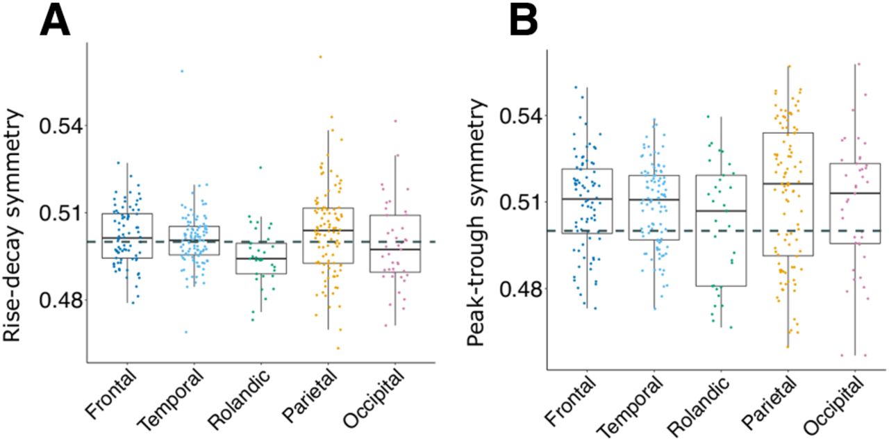
Waveform shape across regions. A, Average rise-decay symmetry for each bipolar recording (indicated as dots), divided by cortical region. B, Same as A, for peak-trough symmetry. Dashed lines indicate 0.5. Overall, cortical sites were symmetrical in rise-decay symmetry (β = 2e-03, t = 1.48), and showed a slight but statistically significant bias for longer peaks than troughs (β = 8e-03, t = 2.92).
Variability in spindle frequency
In addition to spindle frequency varying between regions, we found there was substantial variability across sites within a region, across spindles measured at a single cortical site, and within individual spindles. Here, we compare the magnitude of these sources of variability with our reported average difference between frontal and parietal channels of 0.64 Hz (12.10 vs 12.74 Hz; Table 2).
Frequency variability across sites within a single cortical region
The variation within a region across channels was lower in frontal and temporal cortices, ranging from 0.34 to 0.28 Hz SDs, respectively, compared with parietal and occipital sites ranging from 0.68 to 0.8 Hz, respectively (Table 2; Fig. 2A, boxplot). Notably, the SD across channels within a region is larger at parietal and occipital channels than the average difference between frontal and parietal areas (0.64 Hz).
Frequency variability at a single cortical site
We also assessed whether individual cortical sites are better described as unimodal or bimodal distributions, as previous scalp work has reported multiple peaks at individual scalp locations (Werth et al., 1997). In Figure 4A, we present all patients that had at least three frontal and three parietal channels (six patients) and show average PSDs per region, corrected for the aperiodic component. At this regional level, PSDs appear unimodal in the spindle band. However, spindle activity can appear quite broad, especially in parietal cortex, as seen in patients 1, 5, 12, and 16. In Figure 4B, we compare frontal and parietal PSDs at the individual channel level and see that most channels appear unimodal. To quantify this, we applied two approaches. The first was to estimate the periodic components of the PSDs using the FOOOF package. We found that fitted PSDs for 4/365 channels had two periodic peaks within the 10- to 16-Hz range, though the PSDs for two of these channels appeared broad rather than bimodal. We also assessed for bimodality in the distribution of overall spindle frequency for each channel, as shown in Figure 1F. Silverman's test for bimodality found 14/365 channels rejected unimodality at p < 0.05; however, none survived after correction for multiple comparisons (FDR, p < 0.05). The analysis of PSDs as well as the distribution of overall spindle frequencies at the channel level overwhelmingly support unimodal distributions of spindle frequencies at individual cortical locations.

Spindle PSDs for frontal and parietal cortex. Six patients had at least three frontal and three parietal channels, and the average PSD for all channels for each region are shown in A. These PSDs have been corrected by removing each channel's aperiodic, 1/f trend. Average PSDs are primarily unimodal; however, patients 1, 5, 12, and 16 show quite broad PSDs for parietal cortex. B, PSDs as colormaps with all cortical channels on the y-axis, gray lines separating unique patients, and frequency on the x-axis. Again, power has been corrected by removing the aperiodic component. Channels from patients in A are labeled. This display allows the inspection of each channel's peak frequency and the number of peaks for each channel. The majority of channels appear to show a single peak, and some channels show quite broad peaks (e.g., pt 1).
To further assess how much individual sites vary in spindle frequency, we calculated the SD in overall frequency across spindles at each cortical channel (Fig. 5A; Table 3). Cortical regions significantly varied in their interspindle frequency SD at individual cortical sites (F = 13.54, number of channels = 357). Interestingly, temporal (β = 0.07 Hz, t = 2.92), Rolandic (β = 0.20 Hz, t = 6.46), parietal (β = 0.11 Hz, t = 4.27), and occipital cortex (β = 0.17 Hz, t = 5.41) showed greater interspindle variability than frontal cortex. Also notably, the average interspindle frequency SD is 0.87 Hz in NREM across the cortex (Table 3), which exceeds the reported difference in average frequency between frontal and parietal recordings and is indicated with a black triangle on the scale bars in Figure 5.
Spindle frequency variability
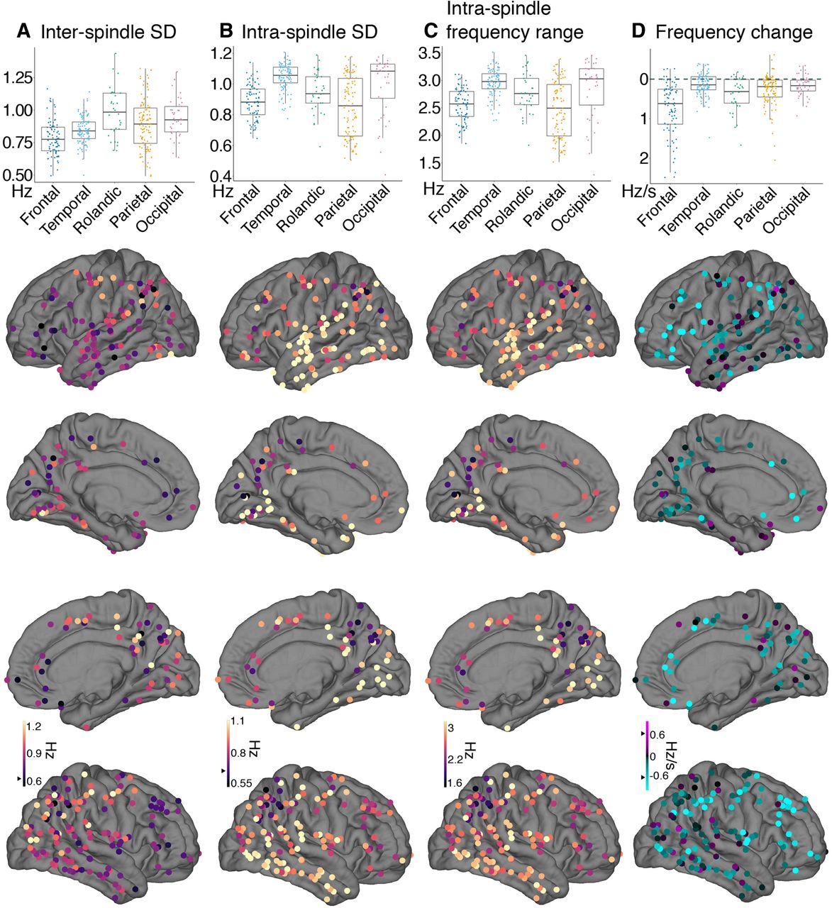
Sources of frequency variability. Cortical bipolar sEEG recordings denoted as circles overlaid on an average surface, with warmer colors indicating greater values. Black triangles mark 0.64 Hz (or Hz/s) to indicate the average difference between frontal and parietal sites. Also shown at the top of the brain surfaces for each measure are boxplots grouped by brain region. A, At individual cortical sites, the SD of overall frequency across spindles in temporal (β = 0.07, t = 2.92), Rolandic (β = 0.20, t = 6.46), parietal (β = 0.11, t = 4.27), and occipital cortex (β = 0.17, t = 5.41) showed greater interspindle variability than frontal cortex. B, The average SD across cycle frequency within a spindle. Temporal (β = 0.14 Hz, t = 5.98) and occipital (β = 0.1, t = 3.6) cortex showed greater intraspindle SD compared with frontal cortex. C, Another measure of intraspindle frequency variation, the average difference between the fastest and slowest cycle within a spindle, is 2.7 Hz on average. D, Average estimated linear change in frequency within a spindle (cyan indicates spindle slowing, pink spindle speeding). Frontal cortex showed significantly more intraspindle slowing than temporal (β = 0.64 Hz/s, t = 9.32), Rolandic (β = 0.35 Hz/s, t = 3.98), parietal (β = 0.47, t = 6.66), and occipital cortex (β = 0.60 Hz/s, t = 6.9). The amount of inter and intraspindle variability often exceeds the observed frontal-parietal overall difference in frequency.
Frequency variability within a spindle
Next, we evaluated measures of intraspindle variability. This includes the intraspindle frequency SD, the range of spindle cycle frequency, and the linear change in frequency. The cortical average intraspindle frequency SD, that is, across spindle cycles within a spindle, was 0.94 Hz during NREM (Fig. 5B; Table 3). This intraspindle variability also significantly varied by cortical region (F = 26.92, number of channels = 357). Both temporal (β = 0.14 Hz, t = 5.98) and occipital (β = 0.1 Hz, t = 3.6) cortex showed greater intraspindle SD compared with frontal cortex. Parietal cortex showed lower intraspindle SD than frontal cortex (β = −0.05 Hz, t = −2.26); however, this difference was not significant after a rank-based transformation that normalized the residuals (t = −1.65). The average frequency range within a spindle, calculated as the difference of the fastest and slowest cycle, was 2.7 Hz (Fig. 5C; Table 3). Like the SD of cycle frequency within a spindle, frequency range also significantly varied by cortical region (F = 23.87, number of channels = 357). Temporal (β = 0.35 Hz, t = 5.75), Rolandic (β = 0.19 Hz, t = 2.36), and occipital (β = 0.29 Hz, t = 3.73) cortex showed greater frequency range than frontal cortex. Similar to intraspindle SD, frontal and parietal cortex were not significantly different for frequency range (original: β = −0.12 Hz, t = −1.88; rank transformed: t = −1.24).
Intraspindle variability is not completely random, but partially reflects a linear change in frequency. Previous work has reported that spindles decrease in frequency during their evolution. However, estimates across the cortex intracranially have not been systematically reported. 45.3% (163/360) of cortical channels showed spindle frequencies that were significantly different at the start versus at the end of the spindle (paired-t test, p < 0.05, FDR adjusted). Of these, 98.2% (160/163) showed slower frequencies at the end versus the start. The three channels that showed faster frequencies at the end of the spindle were located in the lateral inferior temporal sulcus and pericalcarine cortex. For more precise estimates of linear change in frequency, we regressed cycle frequency against time since the first cycle for each spindle (Fig. 1E). The average change estimates across spindles for a given cortical site are displayed for an example channel in Figure 1F, shown for all channels in Figure 5D, and summarized in Table 3. Using this approach, we found that 46.4% of cortical sites had a significant linear change in spindle frequency (one-sample t test, p < 0.05 FDR adjusted), with 95.2% (159/167) showing spindle slowing and 4.8% (eight) channels showing spindle speeding. These eight speeding channels were in the ventral and lateral temporal (two), pericalcarine (two), superior and inferior parietal (two), insula (one), and superior frontal cortex (one) across seven different patients. As evident in Figure 5D, spindle frequency slowing occurred across the cortex, however there was significant regional variability in frequency change (F = 22.99, number of channels = 357). Frontal cortex showed significantly more intraspindle slowing than temporal (0.64 Hz/s, t = 9.32), Rolandic (β = 0.35 Hz/s, t = 3.98), parietal (β = 0.47, t = 6.66), and occipital cortex (β = 0.60 Hz/s, t = 6.9). On average, frontal cortex locations exhibited a decrease of 0.74 Hz/s, yielding ∼0.53-Hz difference from spindle start to end (Table 3). To determine the proportion of overall intraspindle frequency variation that is because of this consistent change in frequency, the observed frequency range within a spindle was compared with an estimated frequency range calculated by multiplying the average duration and frequency change per channel. On average, this estimated range accounted for 12% of the observed frequency range, with 75% of channels accounting for <14%. Thus, the average range in frequency across cycles of a given spindle is about four times larger than the average difference in frequency between frontal and parietal spindles, and only ∼12% of the within-spindle variability is because of superimposed slowing.
Relationships between spindle characteristics
We also investigated the relationships between spindle frequency and other spindle characteristics. We modeled spindle frequency as a function of spindle duration, intraspindle variation, frequency change, amplitude, and high γ power using LMEMs with nested random effects, with observations at the spindle level (Table 4). All variables were entered as fixed effects into a full model with nested random effects for channels within patients. Type II Wald χ2 statistics confirmed each variable provided significant improvement to the model holding all other variables constant. Overall, faster spindles were shorter duration (β= −0.17, SE = 5.4e-03, t = −30.99, number of spindles = 550,475, number of channels = 360, N = 20), showed lower intraspindle SD (β= −0.43, SE = 2.9e-03, t = −147.9), lower amplitude (β = −1.7e-03, SE = 2.3e-05, t = −71.97), greater high γ power (β= 0.23, SE = 3.7e-03, t = 63.3), and more slowing (β = −3.9e-03, SE = 3.9e-04, t = −10.2). We found that these results did not change after controlling for differences because of brain region, sleep stage, or frequency of seizures per patient [Table 5; model specified in Linear mixed-effects models (LMEMs)]. However, although there were statistically significant associations between frequency and other spindle characteristics, the variance explained by each was small (Table 4). We estimated the variance explained in a separate model for each spindle characteristic using the MuMIn R package (Barton, 2020), which provides estimates of the marginal variance explained R2m, or the variance explained by the fixed effects alone, and the conditional variance explained R2c, or the variance explained by both fixed and random effects. The R2m for duration (0.004), intraspindle SD (0.036), amplitude (0.027), high γ power (0.013), and frequency change (6.7e-05) indicate each spindle characteristic only accounts for a small fraction of the variation in frequency. Furthermore, given the average absolute differences of frontal and parietal sites for duration (0.01 s), amplitude (36 µV), intraspindle SD (0.03 Hz), and intraspindle frequency change (0.46 Hz/s), the predicted absolute frequency differences are 0.002, 0.06, 0.013, and 0.002 Hz, respectively, all far lower than the observed 0.64-Hz frontal-parietal frequency difference as well as differences in frequency because of other previously mentioned sources of variability. Hypothesis tests and parameter estimates did not change for individual fixed effects in the full model after transforming spindle frequency with a rank inverse normal transformation and removing residuals that fall outside of ±2 SDs (Table 5). However, because deviation from normality still remained after transformation and outlier removal (Extended Data Table 5-1), we interpret the precise estimates of parameters with caution.
Spindle characteristics explain little variance in overall spindle frequency
Relationship between overall spindle frequency and potential moderators
Extended Data Table 5-1
Assessing normality assumption for the relationship between overall frequency and potential moderators. The top panel shows the original QQ plot, showing a large asymmetric deviation from normality. The data in the bottom QQ plot have been transformed using rank inverse normal transformation, and the overall deviation is lessened but now presents as a symmetric deviation. Download Table 5-1, EPS file.
Epilepsy and spindle frequency
We found no significant effect on overall frequency when adding either measure of epilepsy severity, one based on clinical reports of seizure frequency (high vs low seizure frequency: β = 0.019, t = 0.097 and high vs medium frequency: β = –0.09, t = −0.56) and another based on the proportion of time no intracranial channels were spiking (β = 0.48, t = 0.90). With these measures of individual differences in epilepsy, there is no evidence that epilepsy severity itself explains significant variation in overall spindle frequency.
Spindle co-occurrence
While originally described as a global phenomenon, MEG and intracranial work have identified spindles as primarily local events (Dehghani et al., 2010; Andrillon et al., 2011; Frauscher et al., 2015; Piantoni et al., 2017). We found that indeed the majority of spindles occur at a small proportion of the cortical sites recorded (Fig. 6A,B). Typically, individual spindles occurred in only a single or a few channels, with 50% of spindles occurring in under 16% of channels and 75% in under 25% of channels (on average 18 cortical channels per patient were analyzed for spindles). Frontal and parietal sites showed the greatest proportion of multiple channels participating in spindle events (Fig. 6A). Figure 1C shows an example in one patient of six channels across right frontal and parietal cortex simultaneously spindling. This effect is also clearly shown in Figure 6C, where frontal and parietal sites have the smallest proportion of spindles occurring in only a single channel, and the largest proportion of spindles occurring in four or more channels.

Spindle co-occurrences across the cortex. A, D, Brain surfaces overlaid with cortical sEEG recording sites. Warmer colors indicate greater values. A, The average proportion of channels participating in a spindle at each cortical site; frontal and parietal show the greatest proportion. B, Distribution of the proportion of channels participating in a spindle (top) and absolute number of channels participating in a spindle (bottom) for all spindles from all channels. C, For each region, the proportion of spindles that occurred in one to eight channels. D, For each channel, the proportion of times a spindle initiated a co-spindling event, i.e., when a spindle co-occurred in at least two channels.
We also found that the proportion of spindles that lead or initiated co-spindling events (e.g., spindles detected in multiple channels) was greatest in parietal and especially medial parietal regions (Fig. 6D). In contrast, frontal sites showed the lowest proportion of leading spindles in co-spindle events. During co-spindling events, parietal spindles start earlier than frontal (LMEM; β = −81.75 ms, SE = 12.23, t = −6.68, number of spindles = 427,662, number of channels = 360, N = 20).
Spindles that co-occurred in multiple channels also had unique spindle characteristics. Spindles that occurred in successively more channels were faster in frequency (LMEM with nested random effects for channels within patients; number of spindles = 554,794, number of channels = 365, N = 20; for single channel vs 6+ channels β= 0.36 Hz, SE = 4e-03, t = 86.86), longer duration (for 6+ channels β= 0.13 s, SE = 1e-03, t = 126.86), had lower intraspindle frequency SD (for 6+ channels β= −0.14 Hz, SE = 2e-03, t = −72.98), and showed significantly greater spindle slowing (for 6+ channels β= −0.45 Hz/s, SE = 0.01, t = −31.68). These effects remained significant after controlling for sleep stage and regional differences (Table 6).
Characteristics of widespread spindles
N2 versus N3 differences in spindle characteristics
We compared spindle characteristics between N2 and N3 at the channel level, pooling data from all 20 patients, 357 cortical channels, and 711 unique sleep stage-channel observations and controlled for differences because of brain region. Overall, spindle density was greater in N2 than N3 (LMEM; β = −0.40 spindles/min, SE = 0.04, t = −9.19) and spindles had slightly longer duration in N2 than N3 (LMEM; β = −0.02 s, SE = 2e-03, t = −9.18). There were no significant differences in average spindle amplitude between sleep stages (LMEM; β = 1.15 µV, SE = 0.85, t = 1.35). N2 overall frequency was higher than N3 (LMEM; β = −0.08 Hz, SE = 0.01, t = −5.94) and cortical sites showed a greater interspindle frequency SD for N2 than N3 (LMEM; β = −0.05 Hz, SE = 9e-03, t = −6.17). While there were no differences between N2 and N3 for intraspindle frequency SD (LMEM; β = –5e-03 Hz, SE = 5e-03, t = −0.97), the frequency range was smaller in N3 (LMEM;β = −0.05 Hz, SE = 0.02, t = −3.32). There were no significant differences in rates of change in frequency between N2 and N3 (LMEM;β = –6e-03 Hz/s, SE = 0.03, t = −0.227). Rise-decay symmetry did not differ between N2 and N3 (LMEM; β = 4e-04, SE = 7e-04, t = 0.56); however, peak-trough symmetry was slightly more peak-biased for N3 than N2 (LMEM; β = 18e-04, SE = 7e-04, t = 2.75). N2 sleep showed a greater amount of spindle co-occurrence than N3 sleep (LMEM; β = −0.57 channels, SE = 0.01, t = −94.72, number of spindles = 554 794, number of channels = 365, N = 20). Results did not significantly change with normalizing all data and performing robust regression (Table 7; Extended Data Table 7-1). All significant differences between N2 and N3 survived correction for multiple comparisons (FDR p < 0.05).
Comparing N2 and N3 across spindle features
Extended Data Table 7-1
Assessing normality assumption for the comparison of spindle features between N2 and N3 using LMEMs. Each spindle feature is denoted by a pair of QQ plots, which plot the normal theoretical quantiles by the observed residuals of the model. The left plot of each pair corresponds to the original data, whereas the right corresponds to the data after applying the rank inverse normal transformation (rankit). Because the transformation did not normalize the residuals, we applied a robust LMEM regression which lessens the influence of outliers on parameter estimates. The right plot of each pair shows each observation colored as blue, where brighter blue values indicate datapoints that make larger contributions to parameter estimates and darker colors smaller contributions. All panels show outliers are darker and so contribute the least to parameter estimates. Download Table 7-1, EPS file.
Left versus right hemisphere differences in spindle characteristics
We compared spindle characteristics between left and right hemispheres at the channel level, pooling data from all 20 patients and 357 cortical channels. During NREM sleep, left and right hemispheres did not differ in: spindle density (LMEM; β = −0.14 spindles/min, SE = 0.19, t = −0.73), spindle amplitude (LMEM; β = −5.95 µV, SE = 9.39, t = −0.63), overall frequency (LMEM; β = –3e-03 Hz, SE = 0.07, t = −0.05), interspindle frequency SD (LMEM; β = −0.02 Hz, SE = 0.02, t = −0.81), intraspindle frequency SD (LMEM; β = 0.02 Hz, SE = 0.02, t = 1.12), frequency range (LMEM; β = 0.05 Hz, SE = 0.05, t = 0.97), linear frequency change (LMEM; β = 0.04 Hz/s, SE = 0.06, t = 0.66), rise-decay symmetry (LMEM; β = –6e-04, SE = 16e-04, t = −0.37), nor in peak-trough symmetry (LMEM; β = –4e-03, SE = 2e-03, t = −1.52). We found that spindles occurring in the right hemisphere compared with the left showed greater co-occurrence (LMEM; β = 0.3 channels, SE = 0.1, t = −3.03, number of spindles = 554 354, number of channels = 363, N = 20). The average spindle duration was shorter in left versus right hemisphere (LMEM; β = −0.01 s, SE = 5.5e-03, t = −2.37); however, this effect was not significant after rank inverse normal transformation (β = −0.19 s, t = −1.65) or after correction for multiple comparisons (FDR, p < 0.05). All other measures did not change in significance after normalizing (Table 8; Extended Data Table 8-1).
Comparing left and right hemispheres across spindle features
Extended Data Table 8-1
Assessing normality assumption for the comparison of spindle features between left and right hemispheres using LMEMs. Each spindle feature is denoted by a pair of QQ plots, which plot the normal theoretical quantiles by the observed residuals of the model. The left plot of each pair corresponds to the original data, whereas the right corresponds to the data after applying the rank inverse normal transformation (rankit). This transformation normalizes measures that showed deviation from normality, such as amplitude, NREM density, and frequency change. Download Table 8-1, EPS file.
Cortical-hippocampal spindle phase locking
Previous work found significant phase-locking between hippocampal and cortical spindles for 37% of neocortical channels (Jiang et al., 2019b). The procedure for determining significant phase-locking between hippocampus and cortex is described in Materials and Methods, Assessment of hippocampal-cortical phase-locking value (PLV). An example from one patient in a cortical precuneus channel with significant phase-locking to posterior hippocampus during N3 is shown in Figure 7A, with time 0 indicating the hippocampal spindle start. PLV rises at the onset of the hippocampal spindle and peaks at around 0.4 at 750 ms. A total of 67% of these significant cortical channels were with posterior hippocampus in N2. The latter channels are shown in Figure 7B, with color indicating the peak PLV during N2 with posterior hippocampal spindles. After controlling for differences because of cortical region, the PLV among channels with significant hippocampal-cortical spindle PLV showed a weak positive relationship with overall spindle frequency (LMEM; β = 0.78, t = 1.92, number of channels = 76, N = 12) and a weak negative with intraspindle frequency SD (LMEM; β = −0.2, t = −1.96). Neither spindle duration, frequency change, amplitude, nor N2 or N3 density covaried with PLV after controlling for cortical region (|t| < 1.96; Table 9). After normalizing the data by rank inverse normal transformation of the dependent variable and controlling for region, PLV positively covaried with frequency (LMEM; β = 1.32, t = 2.42; Table 9; Extended Data Table 9-1). However, no associations survived correction for multiple comparisons (FDR, p < 0.05). We previously found 5% of all NC channels showed high NC-HC PLV (peak > 0.4), 70% of which were in parietal channels. Post hoc analyses found after controlling for regional differences, this high PLV subset compared with all other cortical channels were significantly faster (LMEM; β = 0.57 Hz, t = 5.01, number of channels = 341, N = 20; Fig. 7C), had lower intraspindle frequency SD (β = −0.15 Hz, t = −4.7; Fig. 7D), had slightly longer duration (β = 0.02 s, t = 2.82; Fig. 7E), and greater spindle density in N2 (β = 0.77 spindles/min, t = 2.48; Fig. 6F) as well as in N3 (β = 0.72 spindles/min, t = 2.25). These sites did not differ in linear change in frequency (β = −0.1 Hz/s, t = −1.06), interspindle frequency SD (β = 0.03 Hz, t = 0.77), or amplitude (β = −11.74 µV, t = −0.75). These results remained significant after correction for multiple comparisons (FDR, p < 0.05; Table 10). Results did not change after restricting to just parietal channels (LMEM: number of channels = 99, N = 17), except for high PLV sites showing greater spindle slowing (β = −0.24, t = −2.19). Furthermore, results did not significantly change after transforming the dependent variable to normalize residuals (Table 10; Extended Data Table 10-1). After controlling for the effects of sleep stage, hemisphere, and region, spindles occurring at cortical sites with high PLV also showed greater co-occurrence with spindles across multiple cortical sites (LMEM; β = 0.34 channels, SE = 0.13, t = 2.5, number of spindles = 550,769, number of channels = 360, N = 20). These analyses demonstrate sites with large hippocampal-cortical spindle PLV, predominately parietal sites, have unique spindle characteristics compared with other cortical sites after controlling for regional differences, including faster frequency, lower within-spindle frequency variation, longer duration, greater density, and a greater degree of spindle co-occurrence across cortical sites.
Relationship between the max PLV of hippocampal-cortical spindles and spindle features
Extended Data Table 9-1
Assessing normality assumption for the covariation between cortical-hippocampal PLV during spindles and spindle features using LMEMs. Each spindle feature is denoted by a pair of QQ plots, which plot the normal theoretical quantiles by the observed residuals of the model. The left plot of each pair corresponds to the original data, whereas the right corresponds to the data after applying the rank inverse normal transformation (rankit). This transformation normalizes measures that showed deviation from normality, such as interfrequency SD, N2 density, and intrafrequency SD. Download Table 9-1, EPS file.
Comparing channels with high and low hippocampal-cortical phase-locking during spindles
Extended Data Table 10-1
Assessing normality assumption for the comparison of spindle features between cortical channels with high hippocampal PLV during spindles versus those with low using LMEMs. Each spindle feature is denoted by a pair of QQ plots, which plot the normal theoretical quantiles by the observed residuals of the model. The left plot of each pair corresponds to the original data, whereas the right corresponds to the data after applying the rank inverse normal transformation (rankit). This transformation normalizes measures that showed deviation from normality, such as frequency change, N2 density, N3 density, duration and amplitude. Download Table 10-1, EPS file.

Cortical-hippocampal spindle phase locking. A, A cortical precuneus channel from one patient with significant phase-locking during spindles with the posterior hippocampus during N3; time 0 indicates the onset of spindles in the hippocampus. PLV increases after spindle onset and peaks around 0.4 at 750 ms. B, Channels with significant PLV during spindles with a posterior hippocampal channel during N2, as identified by Jiang et al. (2019b), are indicated as circles, with the peak PLV shown in color. Nonsignificant channels are displayed as crosses. Statistical relationships between PLV in significant channels and spindle features are reported in Table 9 and Extended Data Table 9-1. Areas with the highest PLV are apparent in parietal cortex as well as posterior ventral temporal cortex. We performed post hoc analyses comparing these high PLV channels (PLV >0.4) and all other cortical channels, including those with nonsignificant PLV, across several spindle characteristics. Differences between high and low PLV channels in spindle features are reported in Table 10 and Extended Data Table 10-1. C–F, Each dot is a channel, different colors denote different brain regions. High PLV channels were significantly faster (LMEM; β = 0.57, t = 5.01, number of channels = 341, N = 20), (D) had lower intraspindle frequency variation (β = −0.15, t = −4.7), (E) had slightly longer duration (β = 0.02, t = 2.82), and (F) had greater spindle density in N2 (β = 0.76, t = 2.48). These results did not change when restricting to just parietal channels.
Slower and faster spindles show similar coupling to downstates
Putative evidence for dichotomizing spindles as slow or fast includes that they have different coupling to SOs, wherein frontal, slower spindles precede and faster, centro-parietal spindles follow downstates (Mölle et al., 2011; Klinzing et al., 2016); however, recent intracranial work does not support this effect (Mak-McCully et al., 2017; Gonzalez et al., 2018). Studies vary in the cutoff frequency that separates slow from fast spindles, as spindle peak frequencies vary across subjects (Ujma et al., 2015) and some subjects do not show distinct slow and fast spindle peaks in averaged power spectra (Werth et al., 1997; Gennaro and Ferrara, 2003; Mölle et al., 2011; Cox et al., 2017). We chose 12 Hz to demarcate slower and faster spindles, as 12 or 13 Hz is typical (Schabus et al., 2007; Barakat et al., 2011; Mölle et al., 2011; Ayoub et al., 2013), and determined whether there is regional variability in whether slow spindles precede downstates and fast spindles follow.
The polarity of our LFP for detecting downstates was corrected for each cortical channel such that large, low-frequency negative deflections corresponded with high γ power suppression; the grand average across all cortical channels is shown in Figure 8A.

Times of spindles relative to downstate troughs. The polarity of each cortical bipolar recording is corrected such that negative indicates the trough of the DS, as determined by suppression of high γ (70–190 Hz), shown in A as the grand average across all cortical channels. B, An example epoch where spindles are coupled to downstates for a superior parietal channel from one patient. C, For the same channel in B, a histogram of the occurrence of spindles starting around the DS trough. The probability of spindles starting relative to downstates for all channels with spindles that significantly started before or after downstate troughs are shown in D, E. In D, each gray line corresponds to a bipolar, cortical recording, with black lines indicating average across channels and blue lines chance occurrence. E, Each row is a cortical channel, with gray lines separating different patients and magenta lines indicating the time of downstate trough. The y-axis in D and color in E indicate the probability of spindles starting in a particular time bin. For each region, all spindles starting within ±1 s of the downstate trough are included. The most consistent effect across channels is that spindles have the highest probability of starting after the downstate trough, most apparent in frontal and parietal cortex.
An example of spindle activity coupled to slow waves in a superior parietal bipolar sEEG recording from one patient is shown in Figure 8B. Figure 8C indicates when spindles are most likely to start when detected around the time of downstate troughs for the same channel as Figure 8B. We found that of the 365 channels, 320 had at least 40 spindles starting within ± 0.5 s of cortical downstates. There were significantly more spindles starting 0.5 s after downstates compared with starting before (LMEM; β =180.5 spindles, SE = 28.2, t = 6.4, number of channels = 320, N = 20). Of these 320, 208 showed a significant tendency for spindles to start after (77%, 160 channels) or before (23%, 48 channels) downstates (two-sided binomial test; p < 0.05, FDR adjusted). The probability of spindles starting relative to downstate troughs for all regions is shown in both Figures 8D,E. In Figure 8D, gray lines indicate significant channels and black lines regional averages. In Figure 8E, each row is a cortical channel, color denotes the probability of spindles starting, and gray lines separate patients. The most consistent effect across regions is that spindles have the highest probability of starting after downstates, most clear for frontal and parietal cortex. Indeed, the majority of significant sites were from frontal (29%, 60 channels) and parietal (31%, 64 channels) cortex. Significant channels from frontal and parietal sites, regardless of preferred latency, are shown in Figure 9. To compare differences in coupling of spindles to downstates by frequency, only channels with at least 100 spindles <12 Hz and 100 spindles >12 Hz within ±1 s of downstates are shown. Because the sample sizes of spindles <12 Hz and >12 Hz were unbalanced for some channels, we bootstrapped the spindle latency times for both frequency conditions over 10,000 iterations, using the size of the smaller condition. With each iteration, a histogram of spindle start latencies was generated, and the average of these histograms was normalized across bins for each channel (shown as color in Fig. 9A,B). To assess whether there were significant differences between either frequency condition and chance, or between the two conditions, we fit a LMEM on the probability of spindles starting at each time bin and display error bars of SE (Fig. 9C,D). The blue dashed line indicates the probability of spindles starting by chance. Time bins where error bars do not include the chance line indicate significance at p < 0.05. Both spindles >12 Hz (pink triangles) and <12 Hz (gray squares) were more likely to start after downstate troughs compared with chance, and less likely to start before, for both frontal and parietal cortex. Nonetheless, the degree to which spindles preferentially occur after the downstate is less for spindles <12 Hz, especially for parietal cortex. However, whether spindles are overall slower or faster, they show similar temporal relationships to downstates.

Slower and faster spindles more likely to follow than precede downstates. A, B, Cortical channels with at least 100 spindles < 12 Hz and 100 spindles > 12 Hz starting within ±1 s of downstate trough are shown. Rows indicate cortical channels, gray lines separate patients, and the dashed magenta line indicates time of the downstate trough. Color indicates the probability of spindles starting within that channel. For both regions and frequency groups, there is a greater probability of spindles starting after the downstate trough compared with before. This is statistically assessed in C, D, where LMEMs, with patient as random effect, modeled the probability of spindles starting at each time bin for each frequency condition separately, with pink triangles showing spindles >12 Hz and gray squares for spindles <12 Hz. Error bars reflect SE, and the blue dashed line indicates the probability of spindles starting by chance. Time bins where error bars do not include the chance line indicate significance at p < 0.05. Overall, spindles were more likely to start after the downstate trough than before. The degree to which spindles preferentially occur after the downstate is less for spindles <12 Hz.
Discussion
This study uses sEEG recordings to investigate spindle characteristics including multiple sources of variability in spindle frequency. While spindles were detected in all cortex areas sampled, temporo-occipital sites showed lower density, more variable frequency, and shorter duration spindles. Fronto-parietal regions had the greatest spindle duration, density, and proportion of spindles co-occurring in multiple channels; consistent with them making the largest contribution to EEG. Spindle frequency variability was assessed across spindles within a channel, and across cycles within spindles, then compared with fronto-parietal differences. While, compared with frontal channels, we observed faster overall frequency in Rolandic (0.37 Hz) and parietal (0.64 Hz) cortices, the SD across spindles within a site, and across cycles within a spindle, were both larger (0.87 and 0.94 Hz, respectively). We also found that spindles which occurred in multiple channels were faster, showed greater slowing, and had lower intraspindle variability, thus indicating that local spindles differ from more global events. Previous work identified a subset of parietal channels with high phase locking to posterior hippocampal spindles (Jiang et al., 2019b); here, we describe how these cortical sites have spindles with faster frequency, longer duration, lower intraspindle variability, and greater density. Although our findings are from epileptic patients and not a healthy population, we analyzed a large number of patients (n = 20) with unique epileptiform etiologies, had broad cortical coverage, excluded sleep periods or channels with pervasive epileptic activity, and analyzed spindles whose appearance as well as other spindle characteristics such as density were within healthy ranges.
The dichotomy of parietal-fast and frontal-slow spindle types was introduced based on EEG (Gibbs and Gibbs, 1950). However, most intracranial work reports a gradient of spindle frequencies (Peter-Derex et al., 2012; Frauscher et al., 2015; Piantoni et al., 2017), with an exception being Andrillon et al. (2011). Our findings suggest a modification to the model of spindles as dichotomous slow and fast systems. We found individual locations exhibit both faster and slower spindles, and that there is a large overlap in the distribution of frequencies between frontal and parietal sites (Fig. 2A). The width of frequency distributions at individual sites was broader in temporal-Rolandic-parietal-occipital regions than frontal sites (Fig. 5A), as previously reported along medial structures (Andrillon et al., 2011).
In addition to the variability in spindle frequency at individual sites, there is also substantial variability within each spindle. We found the fastest and slowest cycles within a spindle on average differed by 2.7 Hz, greater in temporal-occipital sites, and lower at frontal-parietal (Fig. 5B,C). This variability includes a systematic decrease in cycle frequency over the course of spindles, previously observed with EEG (O'Reilly and Nielsen, 2014; Souza et al., 2016) and MEG (Dehghani et al., 2011a). In our study, we found that 46% of recordings from medial and lateral cortex had a significant change in linear frequency; of these, nearly all (95%) slowed, with an overall average of −0.34 Hz/s, and greatest in frontal cortex at −0.74 Hz/s. In sum, these different sources of variability (interspindle, intraspindle expressed as frequency range, and intraspindle slowing) all vary by cortical region, and in the majority of channels, exceed the net 0.64-Hz frontal-parietal difference (Fig. 5, see black triangles on color bars).
MEG and intracranial recordings have shown that spindles are largely local phenomena (Dehghani et al., 2010; Andrillon et al., 2011; Frauscher et al., 2015; Piantoni et al., 2017). Here, we found most spindles occurred in only a single or a few channels (Fig. 6). Co-occurring spindles apparently underly scalp EEG. Specifically, intracranial work found that scalp spindles were associated with asynchronous σ activity, predominantly at frontal-parietal sites (Frauscher et al., 2015), and simultaneous MEG/EEG found spindles detected in both modalities had a 66% increase in the number of MEG sensors involved in the spindle, especially over frontal sensors (Dehghani et al., 2011b). Similarly, we found that frontal and parietal sites showed the greatest proportion of spindles occurring in multiple channels (Fig. 6C). We also replicated the phenomenon, previously observed at the scalp (Dehghani et al., 2011a; Mölle et al., 2011) and intracranially (Andrillon et al., 2011), that spindles at central-posterior sites precede anterior spindles (Fig. 6D). Furthermore, we found that spindles occurring across multiple channels exhibit faster overall frequency, lower within-spindle frequency variability, and much greater spindle slowing (Table 6). These differences could reflect stereotyped, global propagation patterns, such as rotating waves (Muller et al., 2016). Our finding that parietal spindles precede frontal spindles agrees with the previously observed temporal-parietal-frontal progression of spindle cycles. However, these patterns were identified with electrocorticography and our bipolar transcortical sEEG recordings are unambiguously local but more irregularly spaced across the cortex.
Communication between hippocampal and cortical rhythms could serve as a substrate for restructuring recent experiences into long-term memory. Previous work has shown that ripples in the hippocampus are phase locked to hippocampal spindles (Staresina et al., 2015; Jiang et al., 2019b), which in turn are phase-locked with inferior parietal spindles (Jiang et al., 2019b), in locations that are activated in recollective experiences (Gilmore et al., 2015; Hoppstädter et al., 2015). We found that these cortical sites also had unique spindle characteristics, including faster frequency, lower intraspindle frequency variation, longer duration, and greater density (Fig. 7). We speculate that these spindles could play a unique role in processing detailed, episodic information. Considering spindles at these sites spread more widely, they could coordinate or drive spindle dynamics at other cortical structures.
The assertion that slow spindles precede downstates and fast spindles follow is often cited as evidence for their distinct generating mechanisms (Mölle et al., 2011; Timofeev and Chauvette, 2013; Klinzing et al., 2016). Replicating our previous work (Mak-McCully et al., 2017; Gonzalez et al., 2018), we found that spindles were significantly more likely to start after downstates across cortical sites (Figs. 8, 9). We showed that within the same channels, and in both frontal and parietal sites, spindles above and below 12 Hz both follow cortical downstates (Fig. 9). Faster spindles showed a greater likelihood of initiating after downstates than slower spindles, especially in parietal cortex (Fig. 9C,D). Overall, these findings affirm spindles, regardless of frequency, show similar temporal relationships to downstates and are consistent with slower and faster spindles existing along a continuum instead of arising from distinct neurophysiological generators.
Spindles are generated by an interaction of intrinsic currents (h and T) and local circuits within the thalamus (between reticular nucleus and projection nuclei; Destexhe and Sejnowski, 2003), and are projected to all cortical areas (Mak-McCully et al., 2017). The h and T currents are hypothesized to be de-inactivated by the downstate, thus triggering the spindle (Mak-McCully et al., 2017). Latency data imply that the thalamic downstate is triggered by a preceding cortical and that cortical spindles are triggered by thalamic. Thus, this proposed mechanism would explain the common downstate-then-spindle order observed in the cortex through its interaction with the thalamus.
The variability of spindle characteristics within and between areas surely reflect a large number of factors. The patterns of local spread of cortical spindles imply that although they may be originally triggered by thalamo-cortical projections, they may also be locally generated (Dickey et al., 2021a), and indeed the local circuitry and voltage-gated channels necessary for this are present in the cortex (Kalmbach et al., 2018). Thus, topographical variations in spindle properties could be because of variations in either the thalamus or cortex. Extensive transcriptomic (Burt et al., 2018) and histologic (Amunts and Zilles, 2015) studies have identified variations in the expression of various subtypes of the relevant neurotransmitter synthesis and receptor proteins, as well as the h and T channels in humans between cortical areas. In addition, variability can arise from the changing state of local circuits, synapses and channels. For example, the duration of spindles can be affected by cortico-thalamic feedback (Bonjean et al., 2011). The current study offers quantitative data for testing the possible role of these different factors in spindle variability.
The current study found that spindles vary considerably across multiple characteristics, including duration, amplitude, density, spread, onset, and relation to other sleep waves and structures, as well as in the variability of these characteristics. This variation was observed between individual cycles of spindles, between different spindles recorded from the same electrode derivation, between different electrodes in the same cortical area, and of course between different cortical areas. However, the variation between cortical areas was usually smaller than other sources of variation. Although there was sometimes association between different characteristics, this was not systematic or dichotomous. Thus, in contrast to the conception of spindles as comprising two distinct categories differing in location, frequency, relation to downstates, and presumably all other characteristics, we observe a broad range of characteristics in each structure, electrode, and spindle, with variable relationships. Our data indicates that to the extent that regular differences can be discerned in anterior versus posterior EEG recordings, they reflect the sum of many variable cortical generators rather than two monolithic and uniform generators.
This reconceptualization of spindles as varied and heterogenous has implications for interpreting the finding that fast but not slow spindles are involved in memory consolidation (Barakat et al., 2011; Mölle et al., 2011). However, these studies conflated spindle frequency with sensors (i.e., did not consider faster frontal spindles or slower central-parietal spindles), and dichotomized frequency as either slow or fast. Analyzing memory consolidation as a function of frequency treated as a continuous variable in both frontal and posterior spindles would be needed to examine whether spindle frequency per se moderates learning and memory. Here, we found faster spindles are associated with greater high γ (Table 4) and are more tightly associated with initiating on the down-to-upstate transition (Fig. 9). Since spindles occurring on down-to-upstate transitions are associated with greater calcium influx to layer 2/3 mouse pyramidal neurons, compared with spindles alone (Niethard et al., 2018), faster spindles could result in more calcium influx which is hypothesized to facilitate cortical plasticity. Considering spindles as heterogenous also has implications for using spindles as biomarkers in psychiatric disorders such as schizophrenia (Ferrarelli et al., 2007; Manoach and Stickgold, 2019). For example, deficits in faster spindles would not imply an exclusive targeting of central-parietal sites for observation or treatment.
In summary, we found that both frontal and parietal cortex show large numbers of both “fast” and “slow” spindle cycles, and both types occur mainly following downstates. Other characteristics vary quasi-independently, clearly indicating that cortical spindle generators form a continuum. This reconceptualization may inform future efforts to relate spindles to memory consolidation and clinical disorders.
Footnotes
This work was supported by the National Science Foundation Graduate Research Fellowship DGE-1650112, the National Institute of Mental Health Training Program in Cognitive Neuroscience Grant 5T32MH020002, the ONR-MURI Grant N00014-16-1-2829, NIH grant RF1 MH117155, the Department of Veterans Affairs Office of Academic Affiliations Advanced Fellowship Program in Mental Illness Research and Treatment, the Medical Research Service of the Veterans Affairs San Diego Health Care System/University of California, San Diego, and the Department of Veterans Affairs Desert Pacific Data Science Fellowship within The Mental Illness Research, Education, and Clinical Center. We thank Burke Rosen, Charlie Dickey, Adam Niese, Maxim Bazhenov, and Terrence Sejnowski for feedback and support. We also thank Jacob Garrett for providing a measure of spiking activity, Scott Cole and Tammy Tran for providing assistance and custom code for waveform shape analysis, and Burke Rosen for assistance in channel localization.
The authors declare no competing financial interests.
- Correspondence should be addressed to Christopher Gonzalez at ceg017{at}health.ucsd.edu or Eric Halgren at ehalgren{at}ucsd.edu


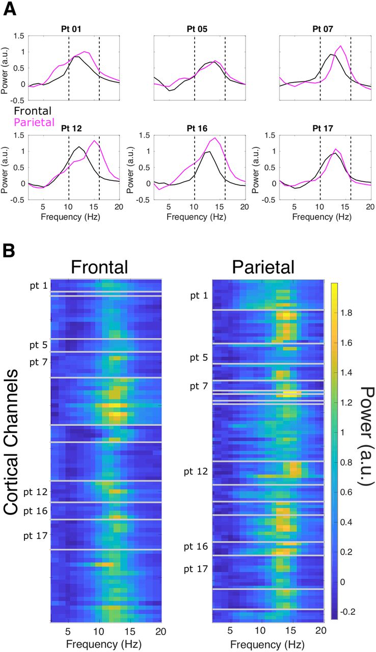