
Abstract
Synchronization of neural activity is fundamental for many functions of the brain. We demonstrate that spike-timing dependent plasticity (STDP) enhances synchronization (entrainment) in a hybrid circuit composed of a spike generator, a dynamic clamp emulating an excitatory plastic synapse, and a chemically isolated neuron from the Aplysia abdominal ganglion. Fixed-phase entrainment of the Aplysia neuron to the spike generator is possible for a much wider range of frequency ratios and is more precise and more robust with the plastic synapse than with a nonplastic synapse of comparable strength. Further analysis in a computational model of Hodgkin–Huxley-type neurons reveals the mechanism behind this significant enhancement in synchronization. The experimentally observed STDP plasticity curve appears to be designed to adjust synaptic strength to a value suitable for stable entrainment of the postsynaptic neuron. One functional role of STDP might therefore be to facilitate synchronization or entrainment of nonidentical neurons.
- synaptic plasticity
- spike-timing dependent plasticity
- synchronization
- entrainment
- hybrid circuit
- dynamic clamp
- neuronal control
Introduction
The synchronization of oscillatory neural activity is a general mechanism underlying transient functional coupling of neurons, the formation of neural ensembles, and large scale neural integration (Laurent and Davidowitz, 1994; Engel et al., 2001; Varela et al., 2001). Two recent examples illustrate this. Simultaneous recordings in the primary motor cortex of monkeys during task performance demonstrate accurate spike synchronization (Riehle et al., 1997). Fell et al. (2001) showed that human memory formation is accompanied by rhinal–hippocampal gamma synchronization followed by a later desynchronization. The observed synchronization becomes more effective and robust as a result of learning (Wagner, 2001).
These observations lead to the following key questions. What are the mechanisms that synchronize neurons with different intrinsic dynamics and frequencies? Why is neural synchronization so robust against noise? Which synaptic features and which features of the postsynaptic neuron are really important for stable synchronization (or entrainment) with fixed phase shift? To answer these questions it is necessary to consider both the cooperative dynamics of large neural ensembles with diverse interconnections and the primary mechanisms of synchronization in minimal neural circuits. In this paper we investigate the second issue preparatory to the large scale computations required for the first.
The mathematical description of neural synchronization or entrainment has a long history, but starting in the late 1980s to the present the role of synaptic dynamics, and in particular synaptic plasticity in neural synchronization, has increasingly attracted the attention of neuroscientists (Doya and Yoshizawa, 1989; Ermentrout and Kopell, 1994; Tsodyks et al., 2000; Bose et al., 2001; Manor and Nadim, 2001; Loebel and Tsodyks, 2002; Karbowski and Ermentrout, 2002; Suri and Sejnowski, 2002). Another recent development is the characterization of spike-timing dependent plasticity (STDP) (Markram et al., 1997; Bi and Poo, 1998, 2001; Abarbanel et al., 2002). In this type of plasticity, a synapse is depressed or potentiated according to the timing of presynaptic and postsynaptic spikes. This led us to the hypothesis that STDP might allow a synapse to adjust to an optimal strength for synchronization.
Our previous modeling with the type of STDP found in the mormyrid electrosensory lobe (Bell et al., 1999) has shown (Zhigulin et al., 2003) that STDP allows synchronization over a much wider range of frequency mismatches and makes it much more robust to noise. These results encouraged us to explore the role of the more common and substantially different type of STDP found, e.g., in rat hippocampus (Markram et al., 1997; Bi and Poo, 1998). In an independent investigation, Karbowski and Ermentrout (2002) showed within the framework of phase oscillators that this type of STDP allows stable and robust synchronization both in minimal circuits and in large heterogeneous networks. In the present work, we analyze the stability and robustness of synchronization in a hybrid neural network [spike generator–dynamic clamp (STDP synapse)–living neuron]. In parallel numerical experiments we simulated two Hodgkin–Huxley (HH)-type model neurons connected by an excitatory STDP synapse. Using both the hybrid circuit and a fully computational model we were able to explore the role in synchronization of various properties of the STDP synapse and of the postsynaptic neuron separately. Full control of the synapse allowed us to probe the role of the specific learning mechanism, whereas the computational model allowed us to test the influence of the properties of the postsynaptic neuron. The hybrid experiment and the model system demonstrate robust fixed-phase entrainment through an STDP synapse.
Materials and Methods
The experiments were performed on Aplysia californica (Kandel, 1976), weighing ∼50–75 gm, that were supplied by the Aplysia Resource Facility (University of Miami, Miami, FL). The animals were kept in a small artificial seawater tank at a temperature of 12°C.
Preparation. The animals were anesthetized with a high concentration Mg 2+ solution injected into the body cavity of the animal at several points. The animal was then opened on the ventral side, and the abdominal ganglion was taken out and pinned to a Sylgard-coated Petri dish. The ganglion was desheathed in the dish on the dorsal side with fine forceps after 5 min application of a few crystals of protease (type XIV; Sigma, St. Louis, MO), washing, and 30 min rest in a hypertonic Mg 2+ solution.
The experiments were conducted in a high Mg 2+, low Ca 2+ saline containing (in mm): 330 NaCl, 10 KCl, 90 MgCl2, 20 MgSO4, 2 CaCl2, and 10 HEPES) that blocks synaptic interaction such that the neurons are effectively isolated.
Experimental setup. Two sharp glass electrodes filled with 3M KCl with ∼10 MΩ resistance were inserted into one tonic spiking neuron on the left side (dorsal side up) of the abdominal ganglion, typically the identified cells L7 or L8. These electrodes were connected to intracellular amplifiers (A-M Systems). One of the electrodes was used to pass the current calculated by a dynamic clamp program and converted by a Digidata 1200 D/A converter (Axon Instruments, Foster City, CA) into the neuron. The other electrode was used to record the membrane potential via an analog-to-digital (A/D) converter (PCI-MIO-16E-4; National Instruments) and the DasyLab (DATALOG) data acquisition software.
The combined spike generator and dynamic clamp software with plastic synapses was developed from a simpler version developed by R. D. Pinto (Pinto et al., 2001) after the original ideas of Sharp (Sharp et al., 1993a,b). It was interfaced with a Digidata 1200 board and run on a Pentium III, 450 MHz system using Microsoft Windows NT 4.0. The presynaptic neuron was simulated by the dynamic clamp software as a simple spike generator with a given generic spike form. The calculated membrane potential of the presynaptic neuron was converted with the Digidata 1200 board as well and recorded on the data acquisition computer simultaneously with the membrane potential of the postsynaptic biological neuron and the injected synaptic current. The setup is summarized in Figure 1.

Experimental setup for the hybrid circuit of a simulated presynaptic neuron, a simulated synapse, and a postsynaptic biological neuron from the Aplysia abdominal ganglion. The presynaptic neuron is a spike generator eliciting spikes of predetermined form at predetermined times that are read from a file. The synapse is simulated by the same software. The calculated synaptic current is injected into the postsynaptic neuron by means of a A/D converter (Digidata 1200; Axon Instruments) and an intracellular amplifier (A-M Systems). The postsynaptic membrane potential is made available to the combined spike generator–dynamic clamp software in the reverse direction. All relevant variables, the presynaptic and postsynaptic potentials, and the injected synaptic current are recorded by a separate data acquisition computer using DasyLab 5.6 (DATALOG). Note that the calculated synaptic current as well as the plastic synapse conductance depend on both the presynaptic and postsynaptic voltages. Through the dependencies on the postsynaptic membrane potential, an effective feedback loop is formed between the synapse and the postsynaptic neuron. This feedback allows the STDP synapse to adjust to the intrinsic properties of the postsynaptic neuron.
Spike generator and synapse model. The combined spike generator and dynamic clamp software generates the presynaptic membrane potential and the synaptic current. The presynaptic membrane potential V1 is calculated from a list of predetermined spike times ti:
 (1) The sum is taken over all spike times ti before the present time t. The spike width used in the experiments was τs = 0.6 msec. The normalized spike potential Vs(t) for a spike with maximum at ti = 0 is given by:
 (2)
(2)
 (3)
(3)
 (4) The variables xa(t) and xb(t) model the rising and falling flank of the spike. The parameter t0 = –0.576 msec was chosen such that the maximum of the potential Vs(t) occurs exactly at t = 0 and xnorm = 3.25394 guarantees that the maximum of Vs(t) is Vspike. In the experiments, this spike amplitude was chosen to be Vspike = 60 mV and the resting potential was Vrest =–40 mV. These are typical values observed in molluscan preparations (compare with data from the Aplysia neuron shown in Fig. 2).
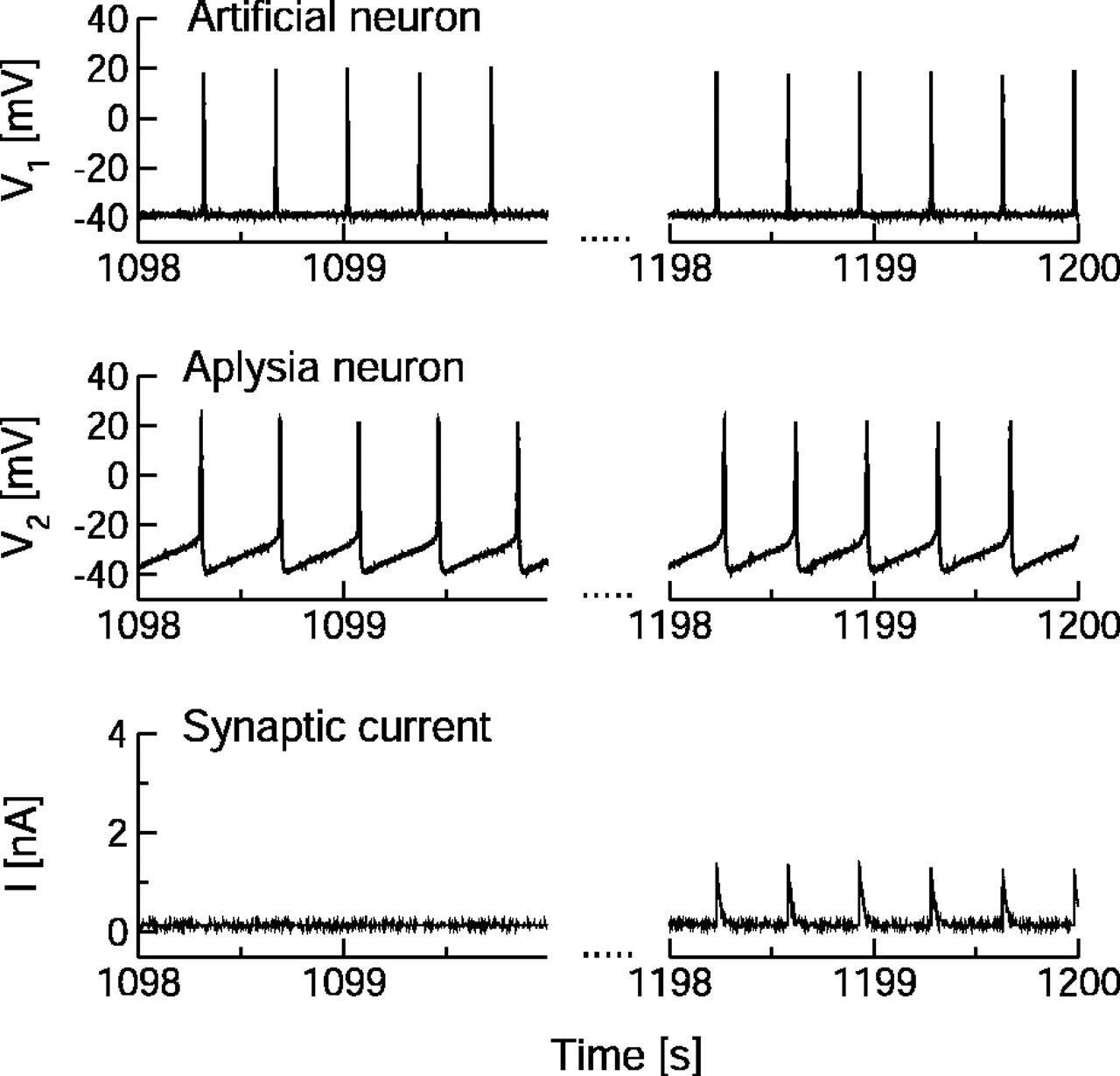
Episode of the uncoupled (left) and coupled (right) dynamics of the simulated and the biological neuron. The coupled dynamics are shown for a situation of stable 1:1 synchronization. The top two panels show the membrane potentials of the simulated presynaptic and the biological postsynaptic cells, respectively. The bottom panels show the synaptic current injected into the postsynaptic neuron. Note the presynaptic and postsynaptic spike forms and the typical EPSCs in the synaptic current. The synaptic strength in this example is comparably weak and clearly stabilized below the allowed maximum gmax.
The synaptic current is a function of the presynaptic and postsynaptic potentials of the spike generator, V1(t), and the biological neuron, V2(t), respectively. It is calculated according to the following model. The synaptic current depends linearly on the difference between the postsynaptic potential V2 and its reversal potential Vrev, on an activation variable S(t), and its maximal conductance g(t):
 (5) The activation variable S(t) is a nonlinear function of the presynaptic membrane potential V1 and has an intrinsic activation time scale τsyn:
 (6) where S∞(V) is a sigmoid function, in particular:
 (7) The reversal potential was chosen to be Vrev = 20 mV, the threshold potential Vth =–20 mV, the inverse slope of the sigmoid function Vslope = 10 mV, and the synaptic time scaleτsyn = 25 msec or sometimesτsyn = 40 msec. The maximal conductance g(t) is determined by the learning rule discussed below. The synaptic current is updated at ∼5–10 kHz depending on how fast the computer is able to evaluate the equations. Figure 2 shows a typical example for the resulting spike forms and synaptic currents.
Learning rule. To determine the maximal synaptic conductance g of the simulated STDP synapse, an additive STDP learning rule with shift was used. To avoid runaway behavior (and resulting damage to the neuron), the additive rule was applied to an intermediate variable graw that then was filtered through a sigmoid function. In particular the change Δgraw in (raw) synaptic strength is given by:
 (8) where Δt = tpost – tpre is the difference in postsynaptic and presynaptic spike times. The parameters τ+ and τ– determine the width of the learning windows for potentiation and depression, respectively, and the amplitudes A+ and A– determine the magnitude of synaptic change per spike pair. The shift τ0 reflects the finite time of information transport through the synapse. Figure 3 (left panel) shows the learning curve for the raw synaptic strength prescribed by Equation 8 for a typical set of parameters.

STDP learning curve (left panel) and filtering curve (right panel). The synaptic conductance g(t) is enhanced if a postsynaptic spike occurs sufficiently long after a presynaptic spike, i.e., Δt is greater than the shift parameter τ0. Otherwise the synaptic strength is depressed. Note that the maximal changes in synaptic conductance occur atτ– +τ0 for depression and τ+ + τ0 for potentiation. The maximally possible changes are A–/e and A+ /e. The specific parameters used in the experiments are given in Materials and Methods. Usuallyτ–= 1.5τ+ and A+ = 1.5 A– were used as shown in this figure. The filtering is used to prevent damage to the postsynaptic neuron if synchronization is not achieved and the synaptic strength could grow without bounds. The filter curve shown in the right panel was generated with the typically used values gmax, gmid = 1/2×gmax and gslope =gmid. Details of the parameters used in the experiments are shown in Table 2.
The raw synaptic strength is then filtered according to:
 (9) The maximally allowed value gmax for g(t) varies in the individual experiments, whereas gmid = ½ × gmax and gslope = gmid were used in all the experiments. By this filtering mechanism it is guaranteed that the maximal conductance g(t) will always have values between 0 nS and gmax. It turns out that the raw synaptic strength graw(t) is already bounded by the dynamics, if the neurons are synchronized, such that this mechanism often is not necessary. For frequency ratios in which entrainment did not occur, however, the bound imposed on g(t) is important to avoid unrealistically high synaptic conductances and possible damage to the postsynaptic neuron. The shape of the filtering function (Eq. 9) is shown in Figure 3 (right panel). Note that in the vicinity of gmid the filtering function is close to the identity function such that it has no serious impact on g and changes in g in this range, i.e., g ≈ graw and Δg ≈ Δgraw in the vicinity of g ≈ gmid. This type of bounding mechanism was chosen over a threshold filter to avoid artifacts arising from positive STDP changes that reach such a threshold and are suppressed followed by negative changes that are not suppressed, thereby destroying the balance between potentiation and depression.
Synaptic changes occur whenever a presynaptic or postsynaptic spike is elicited. The dynamic clamp program continuously detects spikes and memorizes the most recent spike time of each presynaptic and postsynaptic neuron. For each new spike in either of the neurons, the synaptic strength is adjusted according to Equations 8 and 9, immediately taking effect in the next time step of the calculation.
Our implementation of the STDP rule assumes that the experimentally observed rules for isolated spike pairs can be linearly superimposed. Recent results on spike-timing dependent plasticity induced by triplets or quadruplets of spikes (Bi and Wang, 2002; Froemke and Dan, 2002) indicate that a simple superposition of the spike pair-based rule might not always be appropriate. In numerical simulations we therefore also tested a nonlinear superposition scheme based on the suppression model in Froemke and Dan (2002). For more complex spike patterns with very short interspike intervals (ISIs) and therefore a high degree of nonlinear interactions between multiple spikes, a dynamical model of STDP like the one suggested in Abarbanel et al. (2002) might be necessary.
Experimental protocol. For each presynaptic frequency the artificial neuron and the biological neuron were coupled, and their membrane potentials as well as the synaptic currents were recorded for later analysis. In particular, we first took a 100 sec recording of the uncoupled biological neuron and then coupled it to the presynaptic spike generator with an initial coupling strength g0 (this parameter varies over different trials; see results below). The coupling with the plastic synapse was maintained for 100 sec in most of the experiments. Because the intrinsic frequencies of the tonic spiking neurons can vary with the individual preparation, we sometimes also used a shorter coupling period of 50 sec for intrinsically faster neurons. After another 100 sec period of uncoupled recording, we repeated the coupling at a similar frequency but with static synapse strength gstat. Again, we recorded the coupled neurons for 100 sec (50 sec). This procedure was repeated for a set of various presynaptic frequencies. Figure 4 shows an example of a recording from one of the STDP coupling sessions. Table 1 shows the two experimental protocols used for slow neurons (protocol A) and faster neurons (protocol B). To obtain a sufficient number of trials with different frequency ratios, a stable two-electrode recording had to be maintained for 2–3 hr. Not uncommonly, however, one of the microelectrodes slipped or the neuron lost its spontaneous activity. In these cases reinserting the electrode or hyperpolarizing the neuron for a considerable time allowed us to continue the experiment, but it changed the properties of the neuron too much to allow a direct comparison between data collected before and after the adjustments. For analysis, we therefore only included data from “successful” experiments, i.e., experiments in which a full sweep of the relevant frequencies was possible without interruption or loss of stationarity.

Example of a synchronization experiment. The top panel shows the ISIs of the postsynaptic biological neuron and the bottom panel the synapse strength g. Before coupling with the presynaptic spike generator, the biological neuron spikes tonically at its intrinsic ISI of ∼330 msec. Coupling was switched on with g0 = 15 nS at time t = 6100 sec. As one can see the postsynaptic neuron quickly synchronizes to the presynaptic spike generator with ISI 255 msec (top panel, dashed line). The synaptic strength continuously adapts to the state of the postsynaptic neuron, effectively counteracting adaptation and other modulations of the system. This leads to a very precise and robust synchronization at a non-zero phase lag. The precision of the synchronization manifests itself in the very small fluctuations of the postsynaptic ISIs in the synchronized state. Robustness and phase lag cannot be seen directly in this figure.
Experimental protocol for the synchronization assessment experiment
Data analysis. To detect synchronization we first used a simple spike detection algorithm within the DasyLab data acquisition protocol to convert the membrane potential data into interspike interval data. Then we took the ratio of the average interspike intervals of the artificial and biological neuron during the 30 sec before coupling and this ratio for the last 30 sec of the coupled time and plotted these against each other. The choice of averaging over 30 sec was guided by the tradeoff between obtaining good statistics while, at the same time, not averaging over transient dynamics at the beginning of the coupled phase. The coupled ratio as a function of the uncoupled ratio has a form typically obtained for coupled oscillators (Fig. 5). The plateaus in this function correspond to synchronized behavior at the last 30 sec of the coupling phase. The vertical error bars in Figure 5 show the precision of the synchronization, whereas the horizontal error bars show how constant the tonic spiking of the postsynaptic neuron was before coupling. For large variations in ISIs of the uncoupled postsynaptic neuron, stable synchronization to the perfectly periodic artificial neuron cannot be expected.

Two examples of synchronization windows. A and D show the ratios of coupled periods against the ratios of uncoupled periods for the static coupling; B and E display these data for the plastic synapse. Note the much larger synchronization windows and the very small error bars in the synchronized states in the experiments with the STDP synapse. The two experiments shown here correspond to 4 and 5 in Figure 7. C and F show the average synaptic strength of the STDP synapse during the last 30 sec of coupling (triangles) and the constant synaptic strength of the static synapse (circles).
Computational model. To analyze in greater detail how STDP influences the interaction between the presynaptic and postsynaptic neurons we simulated two Hodgkin–Huxley-type model neurons coupled by an excitatory synapse with STDP. Each neuron was modeled using the standard formalism with sodium INa, potassium IK, and leak Ileak currents:
 (10) where i = 1, 2 denotes the number of the presynaptic and postsynaptic neurons, respectively, the leak current is given by Ileak(t) = gleak(Vi(t) – Eleak), and INa(t) IK(t) were (Traub and Miles, 1991):
 (11)Istim is a constant input current forcing each neuron to spike with a constant, Istim-dependent frequency, and the second neuron was driven by the first via the excitatory synaptic current Isyn given by Equation 5. Each of the activation and inactivation variables yi(t) = {ni(t), mi(t), hi(t)} satisfied first-order kinetics:
 (12) The equations for the nonlinear functions αy(V) and βy(V) were:
 (13) and the parameter values were C = 0.03μF, gL = 1μS, EL =–64 mV, gNa = 360 μS, ENa = 50 mV, gK = 70 μS, EK = –95 mV, τSyn = 40 msec.
The time-dependent synaptic coupling strength g(t) was determined by the spike timing of presynaptic and postsynaptic neurons. For each pair of nearest presynaptic and postsynaptic spikes, g(t) changes by Δg(t), which is a function of the time difference Δt = tpost – tpre between the spikes. In the first simulations we used the additive update rule already discussed (Fig. 3 and Eq. 8 and 9) with a linear superposition of synaptic weight changes. The following values of learning curve parameters were used in the simulations: A+ = 9 nS, A– = 6 nS, τ+ = 100 msec, τ– = 200 msec, τ0 = 30 msec. The initial synaptic conductance was taken to be g0 = 20 nS. The parameters were chosen in a way that makes the model neurons to some extent similar to the Aplysia neurons used in the hybrid circuit experiments. Figure 6 shows a typical example of the dynamics of the membrane potentials (top) and the synaptic conductance (bottom). Note the onset of the synchronized state around t = 4000 msec, manifested by the stabilization of the phase difference and of the synaptic strength. In a second set of simulations we repeated the investigation of synchronization with a nonlinear superposition rule, adapted from the results of recent experiments with spike triplets and quadruplets (Bi and Wang, 2002; Froemke and Dan, 2002). In this scheme the changes in synaptic strength depend on the history of previous spike times as well as the relative timing of spike pairs. In particular the simple rule of Equation 8 is replaced by:
 (14) where the total efficacies e1 and e2 are products of efficacies attributable to all previous pairs of spikes:
 (15) where n is the number of the most recent spike of the neuron k and:
 (16) is the “efficacy function.” The index k = 1 denotes the presynaptic neuron, and the index k = 2 denotes the postsynaptic neuron. We used τ1 = 200 msec and τ2 = 500 msec and the amplitudes A+ = 15 nS and A– = 10 nS. All other parameters are chosen as for the linear superposition rule above. The idea behind this type of nonlinear superposition of changes in graw is that the earlier spike pairs dominate and suppress contributions of later pairs. This suppression decays exponentially in time. The underlying assumption in generalizing this rule from spike triplets and quadruplets to continuous spike trains was that the suppression is combined by simple multiplication.

Example of a synchronization experiment in the computational model. The top panel shows the membrane potential of the presynaptic HH neuron (black line) and of the postsynaptic HH neuron (gray line). The bottom panel shows the synaptic conductance. The synchronized state is entered at ∼4000 msec. Note how the synaptic conductance stabilizes at a low value in the synchronized state and that there is a non-zero phase lag of ∼90° in this example.
Results
Frequency synchronization in the hybrid circuit
To detect synchronization we plot the average ratio of the periods of the presynaptic and postsynaptic neuron during the last 30 sec of coupling, 〈(T1/T2)coupled〉, against the average ratio 〈(T1/T2)uncoupled〉 during the last 30 sec before coupling as explained in the data analysis subsection. (T2)uncoupled is the starting period of the postsynaptic neuron. The period of the driving (presynaptic) neuron (T1)uncoupled = (T1)coupled is unchanged when the neurons are coupled because the coupling is unidirectional. The period of the postsynaptic neuron is (T2)coupled when it is driven by the presynaptic neuron. Figure 5 shows two examples.
To compare the quality and range of synchronization in all five successful experiments we calculate three characteristics.
Synchronization window
Synchronization of presynaptic and postsynaptic neurons occurs when (T1/T2)coupled = 1 (Fig. 5). A postsynaptic neuron with a frequency mismatch (T1/T2)uncoupled ≠ 1 was more likely to be entrained by a plastic synapse than a static synapse, as shown by the greater number of points with (T1/T2)coupled = 1 in Figure 5, B and E. To assess the relative success of the static and the plastic synapses, we measured the size of the region in which (T1/T2)coupled = 1. We define the “synchronization window W” as the largest contiguous set of (T1/T2)uncoupled, for which
 is <0.01. The width of this set is denoted by |W|. Note that the data points (T1/T2)coupled are already averages over 30 sec observation time each. We do not propagate the SD of the time average to the average over data points because it is rather a measure of synchronization quality than of synchronization in principle. The quality of synchronization is discussed below. The results for the synchronization window size are shown in Figure 7 (left panel). The synchronization windows for the plastic synapse are always larger than those for the static synapse.

Three characteristics of the synchronization windows observed in five experiments. The left panel shows the width of the synchronization windows, W, the middle panel shows the averaged average ratio 〈〈T1 /T2〉T〉W within the synchronization window, and the right panel shows the averaged SD of the period ratios 〈σ(T1 /T2)T 〉W. The squares are the data obtained with an STDP synapse, and the circles correspond to a static synapse. Note that synchronization windows are always larger and synchronization is always more precise and more robust for the STDP synapse than for the static synapse.
Precision of synchronization
The average ratio 〈〈(T1/T2)coupled〉T〉W over all points within the synchronization window should be exactly 1 for perfect synchronization. Figure 7 (middle panel) shows this average ratio. Note that the values for the plastic synapse are much closer to 1 than the ones for the static case.
Quality of synchronization
The average SD 〈σ(T1/T2)T〉W shows how precisely the neurons were synchronized over the observed time of 30 sec. Figure 7 (right panel) displays this quantity. The quality of synchronization is significantly higher for the STDP synapse.
The parameter values used during the experiments are summarized in Table 2. The strength of the static synapse was chosen to be of the order of the average stationary strength of the STDP synapse to allow a fair comparison. One might be tempted to argue that the synchronization window for the STDP synapse is larger because the static synapse is weaker than the maximally possible value of the STDP synapse. This is not true, as the numerical simulations show (see below). A stronger static synapse shifts the synchronization window toward smaller values of (T1/T2)uncoupled but does not enlarge it (Fig. 8). It would be desirable to demonstrate this effect in the hybrid circuit as well. Unfortunately it is not possible to keep Aplysia cells in a stable condition sufficiently long while driving them extremely hard. Therefore we cannot evaluate static synapses of a strength comparable with the maximal strength of the STDP synapse in the hybrid circuit experiments.
Parameters for the learning and static synapse

Numerical results. Synchronization window for 1:1 frequency synchronization of the simulated neurons for the cases of a static synapse (A, B, D, G) and of an STDP synapse (C, D, H, I). Linear superposition of synaptic changes was used in C and H, and the nonlinear suppression model was used in D and I. Note that the results do not differ significantly. In E and J, the average steady-state value of the synaptic strength g for the STDP synapses and the constant synaptic strength of the static synapses are displayed. The maximal synaptic strength of the STDP synapses was 25 nS in this study. The plots in the right column correspond to simulations with noise. Note the clear enlargement of the synchronization windows for both of the learning schemes and in both presence and absence of noise. The error bars in A–D and F–I indicate the SD of the ratio 〈(T1 /T2)coupled〉. They show the precision of the frequency synchronization. There is a clear dependence of the equilibrium synaptic strength of the STDP synapse in the synchronization regime on the initial frequency mismatch. It can easily be understood because the right side of the synchronization step corresponds to a small initial mismatch and the left side corresponds to a large one. Hence, the forcing needs to be large on the left and small on the right. This is exactly what is observed.
Note that the synaptic strengths for synchronized states, i.e., for points in the synchronization window, are typically weaker than the experimentally allowed maximum gmax. The synaptic strength is bounded by the dynamics alone. Because the filtering function is close to unity for values of g close to gmid, this statement also applies to the raw synaptic strength graw. For frequency ratios that the plastic synapse cannot synchronize, however, the raw synaptic strength typically either grows infinitely or goes to 0 resulting in g being close to gmax or 0, respectively (Fig. 8E,J).
The relationship between the average strength of the STDP synapse within the synchronization window and the presynaptic period T1 (Fig. 8E,J) can be easily explained. Because the frequency mismatch between uncoupled presynaptic and postsynaptic frequency is larger on the left side of the synchronization window, the synapse needs to be stronger to entrain the postsynaptic neuron. On the right-hand side of the synchronization window the frequencies are already very similar in the uncoupled state such that only a very weak synaptic connection is needed for synchronization. Overly strong forcing diminishes the synchrony, as the results for the strong static synapse show (see below).
Numerical results
We studied the synchronization properties of simulated neurons by setting the autonomous (uncoupled) period of the postsynaptic neuron to T2 = 300 msec and then evaluating the average ratio of the periods in the coupled state 〈(T1/T2)coupled〉 as a function of the period ratio before coupling 〈(T1/T2)uncoupled〉. Figure 8 shows 〈(T1/T2)coupled〉 as a function of 〈(T1/T2)uncoupled〉 for the cases of synaptic coupling with constant strength 12.5 nS (A, F) and 25 nS (B, G), synaptic coupling with STDP using the linear superposition rule (C, H), and the coupling with STDP using the nonlinear superposition scheme (D, I). In the STDP cases the steady-state synaptic conductance [lang]g[rang] depends on the ratio of neuronal frequencies (C, F, triangles). Its average overall T1/T2 value is ∼13 nS for both STDP superposition schemes.
Figure 8, A and B, shows the function associated with the 1:1 synchronization domain of a neuron driven by a static synapse. Contrary to naive expectation, the synchronization window is not substantially wider for a stronger synaptic connection; it merely moves further to the left. This is attributable to overexcitation by the overly strong synapse, on the right side of the synchronization window. Figure 8, C and D, shows that the window of synchronization is substantially widened because of the plasticity of the STDP synapse. There does not seem to be a great difference between the two different superposition methods that we used in the STDP rule: both mechanisms show the same widening of the synchronization window. Note that the steady-state conductance of the STDP synapse shown in Figure 8E depends on the mismatch of the presynaptic and postsynaptic frequencies and in most cases is less than its initial value of 20 nS. These results indicate that a plastic synapse enhances neural synchronization by self-adjusting its conductance to the level that is appropriate for a given initial mismatch of the frequencies.
Robustness
We also studied the robustness of this enhanced synchronization in the presence of additive membrane noise and multiplicative synaptic noise. We simulated noise in the membrane potential of the postsynaptic neuron by adding Gaussian white noise to its membrane currents. Multiplicative synaptic noise was implemented by using the following stochastic update rule for the strength g(t) of the STDP synapse. During each update, g(t) was changed by Δgstoch = (1 + R) × Δgraw, where R is a uniformly distributed random number between –0.5 and 0.5. In such a way we ensured that synaptic changes attributable to each event were stochastic, satisfying the learning curve depicted in Figure 3 only on average. This stochastic rule was again implemented both with linear superposition of changes Δg and the nonlinear suppression model.
In the case of the static synapse, we added noise with root mean square amplitude σ = 3 nA (for comparison, peaks of the EPSCs were 0.75 nA in Fig. 8F and 1.5 nA in Fig. 8G) to the postsynaptic membrane and plotted the resulting staircases in Figure 8, F and G. With the STDP synapse we used both membrane noise of the same strength and multiplicative synaptic noise as explained above. Note that the perturbations by additive noise on the membrane potential and the unreliable learning together should have more effect than the pure membrane noise applied to the static synapses. The results are shown in Figure 8, H and I. The synchronization steps in the case of the static synapses are almost completely destroyed by noise, whereas the STDP-mediated synchronization is robust to both membrane noise and synaptic noise.
The mechanism
It is important to understand the mechanisms behind the enhancement of neural synchronization by an STDP synapse. The major factor is that the plastic synapse dynamically adjusts its conductance to a level that is well suited for synchronizing neurons with a given mismatch of intrinsic frequencies. This adjustment is an intrinsic property of the synaptic plasticity that can be understood by a simple stability argument.
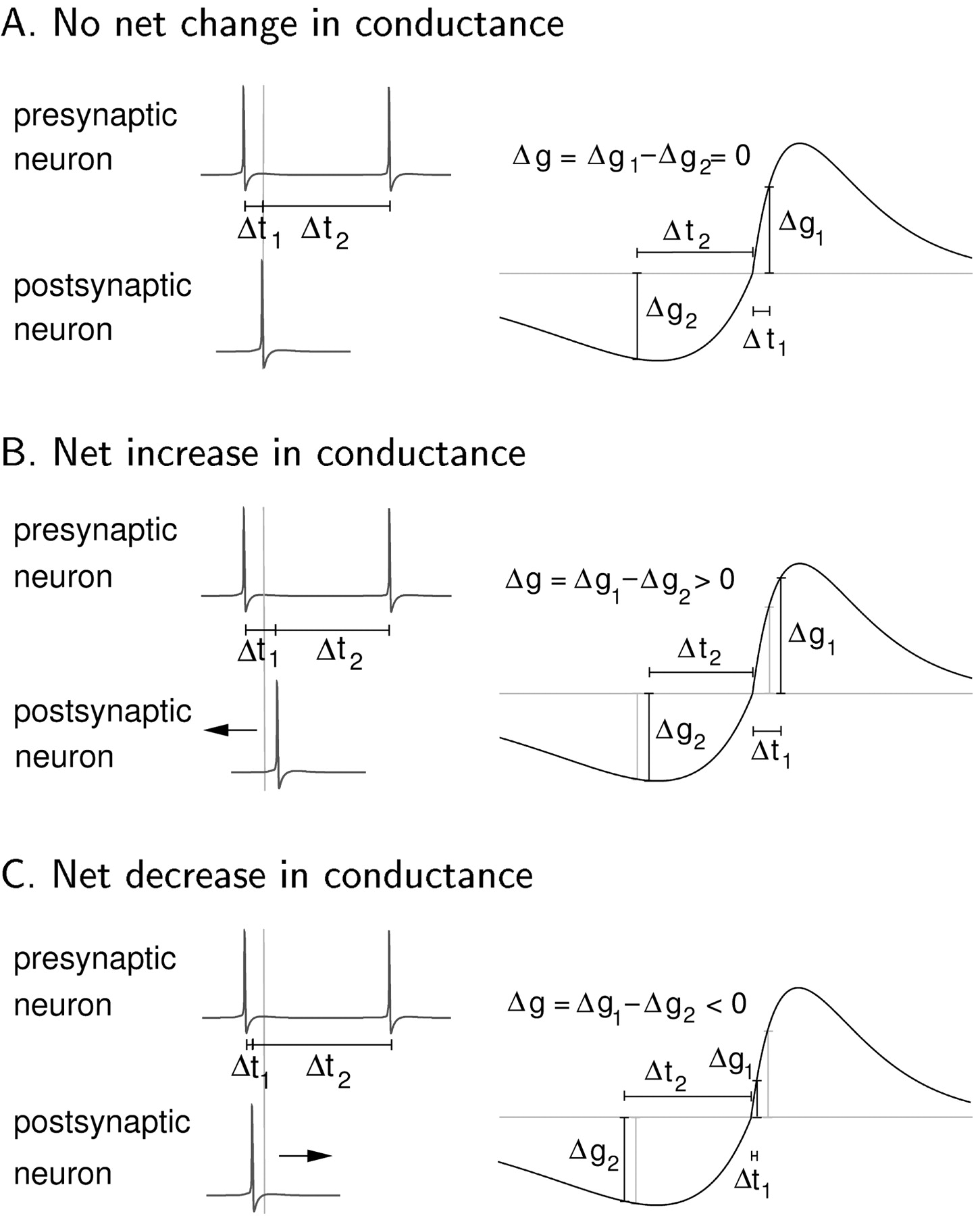
A necessary condition for a stationary synchronized state is that the synaptic conductance is stationary as well. In the situation of two synchronized periodic spike trains with synchronization ratio 1:1 there are two types of contributions to changes in synaptic strength. One stems from the spike pairs composed of a presynaptic spike followed by the next postsynaptic spike. The other is the change determined by the spike pair of the postsynaptic spike and the next presynaptic one (Fig. 9). The synaptic conductance is stationary if these contributions cancel each other such that the total change in synaptic strength after one period is 0.

Mechanism of stable synchronization. A shows the stable fixed point for the synaptic conductance for a period T1 = T2 = Δt1 + Δt2. The two contributions Δg1 and Δg2 cancel each other, and the net change of synaptic strength is 0. If the postsynaptic neuron is too slow as shown in B, the synaptic changes do not cancel such that there is a net increase in synaptic strength, and the postsynaptic neuron is driven stronger forcing it back into the synchronized state. On the other hand, if the postsynaptic neuron is too fast as depictedin C, the net change in synaptic strength is negative, and the postsynaptic neuron is driven less strongly, bringing it back into synchronization as well.
The corresponding time lags Δt1 and Δt2, where Δt1 +Δt2 = T1 = T2, can easily be deduced directly from the learning curve (Fig. 9). To understand why this fixed point for the synaptic strength determines a stable synchronized state for the full system, consider the thought experiment illustrated in Figure 9B. Assume that the neurons are synchronized but the next spike of the postsynaptic neuron is delayed as it tries to break out of the synchronized state. This results in a net increase in synaptic strength driving the neuron back into synchronization. The other direction works in the same way. If the postsynaptic neuron advances its next spike, the net change in synaptic strength is negative; the neuron is less excited and goes back into the synchronized state (Fig. 9C). This analysis assumes a positive phase-response curve for the postsynaptic neuron in the relevant phase regions. This condition is true for both the Aplysia neurons (Kandel, 1976) used in experiments and the HH-type model neurons used in the numerical work.
The time lag of the postsynaptic neuron with respect to the presynaptic neuron resulting from the above analysis is shown as the solid line in Figure 10A in comparison to the observed lags in numerical simulations (triangles). The match between theory and simulation confirms the validity of our analysis; note that the simple HH-type model used in the computational work, apart from overall time scales, was not specifically adjusted to match characteristics of the Aplysia neurons. This clearly shows that the particular spike form of the postsynaptic neuron does not play a major role in this type of synchronization; however, the effect of slow currents and adaptation in the postsynaptic neuron might merit further investigation.

Time lags in the synchronized state. A shows the spike time difference between each presynaptic and the next postsynaptic spike in the synchronized state. The solid line corresponds to the time difference predicted by the fixed point analysis of the learning rule. There is a perfect correspondence in the 1:1 synchronization region. The on average stronger forcing through the static synapse causes on average shorter time delays (B). The dependence of the average time delays on the presynaptic period T1 in the case of the static synapse comes about because the mismatch of frequencies is higher on the left side than on the right side of the synchronization step. Therefore, stronger forcing would be needed to obtain the same small delays on the left side as on the right side, which cannot be provided by the synapse of constant strength.
Discussion
Spike-timing dependent plasticity is a mechanism that enables synchronization of neurons with significantly different intrinsic frequencies. This is a quite unexpected result from our experiments with hybrid circuits and from the computational analysis. These results have yet to be confirmed with real biological synapses that exhibit STDP such as synapses found between hippocampal cells in rats. We will address this question in future work.
Furthermore, STDP-mediated synchronization is a remarkably robust phenomenon. We showed that it is stable against strong noise in the membrane potentials and synaptic processes as well as against a wide variability of the membrane properties of the coupled neurons. This robustness is a result of the dynamic modifications of the synaptic conductance that allow the system to adapt continuously to an optimal state for synchronization. As shown above, the modifications in synaptic conductance arise as a result of the interplay between potentiation and depression. The form of the plasticity curve is such that the resulting synaptic changes keep the postsynaptic neuron stably entrained by the presynaptic neuron at all times. The details of the fast intrinsic dynamics of the postsynaptic neuron do not seem to play a major role in this mechanism. The main characteristics necessary for the successful synchronization are a positive phase-response curve and stationary dynamics. Neurons with slow time scales caused by slow currents or adaptation will need further analysis.
Another consequence of the interplay between potentiation and depression is a dynamic stabilization of the synaptic conductance. It has been shown by several groups that additive STDP learning rules, by themselves, lead to either an unbounded growth or an unbound decay of synaptic strength (Song et al., 2000; van Rossum et al., 2000; Kempter et al., 2001; Rubin et al., 2001; Song and Abbott, 2001). To achieve stability of the learning dynamics, multiplicative rules (Rubin, 2001; Suri and Sejnowski, 2002), learning curves with a negative total integral (Kempter et al., 2001), or, most commonly, artificial bounds on the strength of the synapse (Song et al., 2000; van Rossum et al., 2000; Song and Abbott, 2001) have been used. In contrast to these approaches, we were able to show that the additive STDP learning rule of the type described here results in a self-limitation of synaptic strength that does not require artificial bounds or a negative integral of the learning curve. This is already a quite interesting result on its own.
The main functional role of STDP in neural systems is still not completely clear. In this work we investigated its importance for correlating rhythmic activity of neurons. Because the details of the temporal dynamics of STDP synapses are not known, we have used a phenomenological, instantaneous and deterministic model that is inspired by the experiments of Markram et al. (1997) and Bi and Poo (1998). The changes of synaptic strength that depend on the presynaptic and postsynaptic spiking have been measured in such experiments by averaging over the action of many events that are well separated in time. As a result of such processing one might think that STDP is a slow process and characterized by a long transient time. On the contrary, we think that because the results of individual events can be recognized even after long times (on the order of minutes), it seems evident that information about the timing of spikes needs to be kept in the synaptic dynamics immediately after the event (i.e., after tens of milliseconds). The averaged statistical results just tell us that not all single events are successful such that the average might change on a slower time scale only. Because in our experiment we are interested in the temporally local adaptivity of the synapse and not in long-term plasticity, this is not important, and the use of instantaneous STDP updates is justified.
The learning curve used in this work is slightly different from those used in most computational studies of STDP (Song et al., 2000; van Rossum et al., 2000; Song and Abbott, 2001). The curve that is typically used consists of two exponentials (on the left and on the right from Δt = 0) and is discontinuous at Δt = 0; however, we used a curve that is continuous everywhere. Although available experimental data (Bell et al., 1997; Bi and Poo, 1998; Zhang et al., 1998; Feldman, 2000) are not conclusive as to which type is correct, we argue that a continuous curve appears to be more reasonable from a biophysical point of view. In fact, recent biophysical models of STDP (Abarbanel et al., 2002; Karmarkar and Buonomano, 2002; Whitehead et al., 2003) predict a continuous learning curve, and such curves have been used extensively in a number of phenomenological models (Kempter et al., 2001; Rao and Sejnowski, 2001). It turns out that this type of learning curve is also more suitable for the mechanism of stable neural synchronization investigated here.
In addition to being continuous, the learning curve used in this study also was shifted to the right by a constant time shift τ0. The necessity for this time shift arose from the finite transmission time of the STDP synapse. Because of this finite transmission time, the action of a presynaptic spike onto the postsynaptic activity is delayed. As a result the postsynaptic neuron cannot be driven with a zero phase lag. The learning rule therefore needs to allow a stable synchronized state with an appropriate non-zero phase lag. This was achieved through the shift τ0. We are not aware of hard experimental evidence for such a shift, but because we are injecting currents and measuring potentials at the soma we argue that the time shift in the learning curve merely reflects the backpropagation time of the postsynaptic action potential into the dendrite such that an unshifted learning curve applies at the synapse itself. Note that the shift is comparatively small (Fig. 3) and therefore difficult to detect in noisy experimental data.
The comparison between a simple linear superposition of synaptic changes and the nonlinear depression model adapted from Froemke and Dan (2002) and Bi and Wang (2002) showed no major differences for synchronization. For continuous periodic spike trains like those used in this study, the nonlinear superposition model results mainly in a frequency-dependent depression of the plasticity. The balance between potentiation and depression, which is the important factor for the synchronization mechanism, is not very affected by this depression of plasticity. Therefore it was not unexpected that the impact of the nonlinear superposition scheme on the synchronization results is not significant.
The synchronization observed in this work in both of the experiments with a hybrid circuit and in computer simulations always occurs with non-zero time lag between presynaptic and postsynaptic spikes as mentioned above (Fig. 10). This time lag is determined solely by the STDP learning curve as that time lag that produces no net change in synaptic conductance. It therefore is the same for both the experiments and the numerical work and does not depend on the details of the fast dynamics of the postsynaptic neuron. Its magnitude as compared with the period of oscillations is usually quite substantial; thus the synchronization discussed here is not to be confused with a zero time-lag frequency locking. In different contexts, it has also been referred to as entrainment of the postsynaptic neuron by the presynaptic one.
Our results are in agreement with the earlier theoretical results on heterogeneous networks of phase oscillators mentioned in the Introduction (Karbowski and Ermentrout, 2002). It is worth-while, however, to note some differences in the details. Although synchronization in the symmetrically connected phase oscillator networks show zero phase locking, we always observe a non-zero phase lag stemming from the finite time scale of the synapse dynamics and the unidirectional coupling. The other main difference is the automatic adjustment of synaptic coupling strength to a suitable value for any frequency mismatch. The coupling strength, to some extent, needed to be adjusted to the frequency mismatch by hand in the earlier work (Karbowski and Ermentrout, 2002).
Although concentrating on a minimal neural circuit of two neurons in the present work, the results that we have obtained have profound implications for larger networks of neurons as well. We expect that in the context of larger neuron groups we will be able to observe even more striking effects. We expect that only a few STDP synapses from a “command neuron” might be enough to entrain large ensembles of quite heterogeneous and only weakly coupled neurons. Similar effects have already been observed in the aforementioned work on phase oscillator networks (Karbowski and Ermentrout, 2002). Our own preliminary numerical results also confirm this speculation. It may have implications for the binding problem and even might play a role in epilepsy. In the context of propagating waves in neural networks with STDP synapses such as so-called synfire chains (Abeles, 1991) in the hippocampus, we can predict that the non-zero time lag will determine the properties of the wave, especially its propagation speed.
Footnotes
- Received June 16, 2003.
- Revision received August 19, 2003.
- Accepted August 25, 2003.
This work was partially supported by United States Department of Energy Grants DE-FG03-90ER14138 and DE-FG03-96ER14592, National Science Foundation Grants EIA-013708 and PHY0097134, Army Research Office Grant DAAD19-01-1-0026, Office of Naval Research Grant N00014-00-1-0181, and National Institutes of Health Grant R01 NS40110-01A2. We thank Attila Szücs for helpful remarks and his kind cooperation in an early stage of this work, Reynaldo Pinto for his permission to use and modify his dynamic clamp source code, and Julie Haas for helpful comments.
Correspondence should be addressed to Thomas Nowotny, Institute for Nonlinear Science, University of California San Diego, 9500 Gilman Drive, La Jolla, CA 92093-0402. E-mail: tnowotny{at}ucsd.edu.
Copyright © 2003 Society for Neuroscience 0270-6474/03/239776-10$15.00/0
* T.N. and V.P.Z. contributed equally to this work.