
Abstract
Although our understanding of the mechanisms underlying motor adaptation has greatly benefited from previous computational models, the architecture of motor memory is still uncertain. On one hand, two-state models that contain both a fast-learning–fast-forgetting process and a slow-learning–slow-forgetting process explain a wide range of data on motor adaptation, but cannot differentiate whether the fast and slow processes are arranged serially or in parallel and cannot account for learning multiple tasks simultaneously. On the other hand, multiple parallel-state models learn multiple tasks simultaneously but cannot account for a number of motor adaptation data. Here, we investigated the architecture of human motor memory by systematically testing possible architectures via a combination of simulations and a dual visuomotor adaptation experimental paradigm. We found that only one parsimonious model can account for both previous motor adaptation data and our dual-task adaptation data: a fast process that contains a single state is arranged in parallel with a slow process that contains multiple states switched via contextual cues. Our result suggests that during motor adaptation, fast and slow processes are updated simultaneously from the same motor learning errors.
Introduction
Recent studies support the hypothesis that motor adaptation to external perturbations such as force-field, saccadic gain shift, and visuomotor transformation occurs at multiple timescales (Kojima et al., 2004; Hatada et al., 2006; Smith et al., 2006). To account for this multi-timescale adaptation, Smith et al. (2006) proposed a two-state model, in which a fast process contributes to fast initial learning, but forgets quickly, and a slow process contributes to long-term retention, but learns slowly. This model successfully accounts for a number of adaptation phenomena, including savings, wherein the second adaptation to a task is faster than the first (Kojima et al., 2004); anterograde interference, wherein learning a second task interferes with the recall of the first task (Miall et al., 2004); and spontaneous recovery, wherein if an adaptation period is followed by a brief reverse-adaptation period, a subsequent period in which errors are clamped to zero causes a rebound toward the initial adaptation (Smith et al., 2006).
How these proposed fast and slow processes are organized, however, is ambiguous. Because the two-state model is linear, it can account for the above data with either a serial organization, in which the fast process updates its state from motor errors and sends its output to the slow process, or a parallel organization, in which both the fast and slow processes simultaneously update their states from errors (Smith et al., 2006). Furthermore, such two-state models cannot explain dual- or multiple-task adaptation, because sufficient adaptation to a new task overrides adaptation of a previous task in such models. When given contextual cues and sufficient trials, humans can simultaneously adapt to two opposite force fields (Osu et al., 2004; Nozaki et al., 2006; Howard et al., 2008), two saccadic gains (Shelhamer et al., 2005), or several visuomotor rotations (Imamizu et al., 2007; Choi et al., 2008). The MOdular Selection and Identification for Control (MOSAIC) model (Wolpert and Kawato, 1998) naturally accounts for dual or multiple adaptation via nonlinear switching among multiple parallel internal models. However, because MOSAIC uses only a single timescale for learning and no forgetting (that is, it does not contain distinct fast and slow processes), it cannot explain large increases of errors at the beginning of each block in a dual-adaptation experiment with alternating blocks (Imamizu et al., 2007) or phenomena such as spontaneous recovery.
Here, we systematically addressed the following two questions: Are the proposed fast and slow processes arranged serially or in parallel? Is there one state or more than one for each proposed fast and slow process? Systematic simulations of motor adaptation of candidate models in different adaptation experimental paradigms show that only two models, one parallel and one serial, both with a fast process with one state and with a slow process with multiple states that are switched nonlinearly by a contextual cue, can account for all simulated data. To further differentiate between these two models, we then designed a visuomotor rotation experiment and compared dual adaptation in healthy human subjects to dual adaptation predicted by the serial and the parallel models.
Materials and Methods
Twelve right-handed healthy subjects (seven men, five women, 23–33 years of age) signed an informed consent to participate in the study, which was approved by the local Institutional Review Board. Subjects sat in front of a liquid crystal display monitor and held a joystick. At each trial, subjects moved a cursor to a target by using the joystick. At the beginning of a trial, a cursor appeared at the center position. Two seconds later, a target appeared at one of four positions of the screen (top, right, left, and bottom) 15 cm from the center, and the cursor disappeared. Subjects had 2 s to move the cursor to the target without visual feedback of the cursor trajectory. To provide feedback of performance, the cursor then appeared again for 1 s at a position 15 cm from the center along the direction of the final cursor position. Intertrial intervals were varied randomly from 2 to 14 s. At each trial, we measured the directional error between the target direction and the final cursor direction from the initial cursor position. When subjects did not move within 2 s in a trial, the trial was regarded as a missed trial, and the next trial started.
In the training session, we altered the mapping between the joystick and cursor directions using four different visuomotor rotations (Krakauer et al., 1999, 2005; Wigmore et al., 2002; Miall et al., 2004; Hinder et al., 2007; Seidler and Noll, 2008): 25° (task A), −25° (task B), −50° (task C), and 50° (task D). For subjects to distinguish between the different tasks, we used target positions as a contextual cue: targets for each of four visuomotor rotation tasks appeared at one of four different positions (top, right, left, and bottom). The cue positions were counterbalanced across subjects. In the first 100 trials of the training session, subjects practiced tasks A and B in a massed schedule, which consisted of three consecutive blocks of 50 trials of task A, 25 trials of task B, and 25 trials of task A. In the second 100 trials of the training session, subjects practiced tasks C and D in a pseudorandom schedule: in every two-trial block, one of two tasks was chosen randomly and presented followed by the other task.
In our experiment, we used the A–B–A paradigm as a massed schedule in the first half of the training session for two reasons. First, such a paradigm has been widely used in previous motor adaptation studies (Brashers-Krug et al., 1996; Miall et al., 2004; Krakauer et al., 2005). Second, it is the simplest schedule that allowed us to estimate model parameters reliably with small confidence intervals (see Fig. 6).
Before the training session, subjects performed 200 trials of a baseline session, in which there was no rotation and targets appeared at the four positions in a pseudorandom order.
Candidate models.
We searched for the most parsimonious model that can simultaneously account for all the following motor adaptation data: savings, spontaneous recovery, anterograde interference, and dual adaptation in both blocked and random schedules. We modeled motor adaptation via the summation of the multiple internal states, each modeled with a linear differential equation (see below) with a learning term and a forgetting term (Smith et al., 2006). We studied all possible models with either a serial or a parallel organization of the fast and slow processes, in which each process contains either a single state or multiple states. Furthermore, although previous experiments and modeling studies are consistent with the idea that motor adaptation occurs at multiple timescales rather than at a single timescale (Kojima et al., 2004; Hatada et al., 2006; Smith et al., 2006; Kording et al., 2007; Criscimagna-Hemminger and Shadmehr, 2008; Ethier et al., 2008), we also studied models with a single process with either a single state or multiple parallel states for the completeness of comparisons.
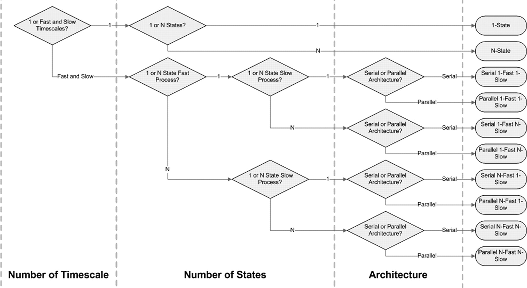
Such systematic search led to 10 different possible models (Fig. 1): (1) a 1-state model, (2) a serial 1-fast–1-slow (1-fast 1-slow) model, (3) a parallel 1-fast 1-slow model, (4) a parallel n-state model, (5) a serial n-fast n-slow model, (6) a parallel n-fast n-slow model, (7) a serial 1-fast n-slow model, (8) a parallel 1-fast n-slow model, (9) a serial n-fast 1-slow model, and (10) a parallel n-fast 1-slow model.

Ten possible motor adaptation models that address the following three questions: (1) Are there slow and fast timescales? (2) Is there one state or more than one for each timescale? (3) Are the fast and slow processes arranged serially or in parallel?
The 1-state model and the parallel and serial 1-fast 1-slow models are identical to those proposed and studied by Smith et al. (2006). For all other models, we added multiple inner states in either the fast or the slow process or both. The differential equations for all states within a process have the same parameters, but the states receive different contextual cue inputs. As in MOSAIC, the contextual cue input has two roles: it selects the appropriate state(s) to be summed in the total output, and it allows the updating of this selected state(s) from motor errors. Forgetting is not gated by the contextual input (see model equations below). For the sake of simplicity, we make the following assumptions: (1) no interference between multiple states, (2) perfect switching between multiple states, and (3) identical learning and forgetting rate parameters for all states within a process. Thus, except for the 1-state model and the parallel n-state model, which contain only two parameters (one forgetting rate A and one learning rate B), all models contain four parameters: one forgetting rate and one learning rate for each fast and slow process (Af, Bf, As, and Bs) (model parameters are given below).
For all models, at each trial n, the motor error input e is determined by the difference between an external perturbation f and the motor output y as follows:
 For the 1-state model, the state update equation is simply given by the following:
 and
and
 where x is a learning process with a single state, A is a forgetting rate, and B is a learning rate.
In the 1-fast 1-slow models, the fast and slow processes have a single inner state each. The state update rules for the parallel representation of the 1-fast 1-slow models are thus given by the following (Smith et al., 2006):
 and
and
 where xf and xs are a fast and a slow learning process with a single state, respectively.
In the parallel n-state model, there is only one process, which has multiple inner states, as follows:
 and
and
 where x is a learning process with Ntask internal states and c is the contextual cue. These two variables are vectors of length Ntask, equal to the number of tasks in the experiment. Because we assumed no interference and perfect switching among internal states in a process, we used a unit vector for c. For example, for the first task, we used c = (1,0,… ,0)T, for the second task, c = (0,1,… ,0)T, and so on.
In the n-fast n-slow models, both the fast and slow processes have multiple inner states (and thus both receive a contextual cue input). The state update rules for the parallel representation of the n-fast n-slow models are thus given by the following:
 and
and
 where xf and xs are fast and slow processes with Ntask internal states.
The parallel 1-fast n-slow model (Fig. 2A) has a fast and a slow process organized in parallel, with a single state in the fast process and multiple states in the slow process. The state update rules for the parallel representation for this model are given by the following:
 and
and
 Similarly, in the parallel n-fast 1-slow models, only the fast process has multiple inner states. The state update rules for the parallel representation of the n-fast 1-slow models are as follows:
 and
and
 All serial models are identical to their parallel counterparts except that the slow process does not receives the motor error input e directly but receives the output of the fast process xf. For example, the state update rule of the slow process for the serial representation of the 1-fast n-slow model is as follows (compare with Eq. 11):
 Finally, it should be noted that we attempted to model the common neuronal mechanism of motor adaptation as in the work of Smith et al. (2006) or Kording et al. (2007) but not the mechanism of specific type of motor adaptation. Therefore, our model does not account for the effect of physiological factors, such as muscle mechanics, limb dynamics, etc.

The two possible architectures of the 1-fast n-slow model: parallel (A) and serial (B). e is a motor error, c is a contextual cue, and x is a motor output. Multiple boxes in the slow process represent internal states switched by the contextual cue input.
Simulation parameters.
Here, we chose parameters for all models to reproduce previous experimental results qualitatively. Note, however, that the simulation results are not limited by these particular parameter values. These qualitative results are valid across wide ranges of parameters (for details, see supplemental material, available at www.jneurosci.org). The parameters of the serial models were determined such that these models behave identically to the corresponding parallel models in massed schedules (see supplemental material, available at www.jneurosci.org).
In the simulations of spontaneous recovery (Fig. 3) and anterograde interference (Fig. 4), we used the parameters given by Smith et al. (2006): Af = 0.92, As = 0.996, Bf = 0.03, and Bs = 0.004 for the parallel 1-fast 1-slow, n-fast 1-slow, n-fast n-slow, and 1-fast n-slow models. For the serial 1-fast 1-slow, n-fast 1-slow, n-fast n-slow, 1-fast n-slow models, we used the following parameters: Af = 0.92, As = 0.996, Bf = 0.0337, and Bs = 0.0091. For the 1-process model and parallel n model, we used A = 0.996 and B = 0.004.

Simulation of spontaneous recovery for all 10 models considered: 1-state model, parallel n-state model, serial and parallel 1-fast 1-slow models, serial and parallel n-fast 1-slow models, serial and parallel n-fast n-slow models, and serial and parallel 1-fast n-slow models. A, Schedule of the error-clamping paradigm used to induce spontaneous recovery, which consists of 180 trials for adaptation to one stimulus (1), 20 trials for adaptation to the opposite stimulus (−1, deadaptation), and 50 error-clamping trials, during which errors are clamped to zero. B, Model predictions of adaptation performance for all models. The parallel and serial models are superimposed in all panels except for the 1-state and parallel n-state models. Check marks or crosses are used to show which models account or do not account for the data, respectively. All models except the 1-state and parallel n-state model can reproduce the characteristic of spontaneous recovery: the output for the first error-clamping trial starts near the baseline (zero), increases trial by trial, and decays slowly.

Simulation of anterograde interference for the eight remaining candidate models: serial and parallel n-fast n-slow models, serial and parallel 1-fast 1-slow models, serial and parallel n-fast 1-slow models, and serial and parallel 1-fast n-slow models. The parallel and serial models are superimposed in all panels. A, Schedule of the A–B–A paradigm used to induce anterograde interference, which consists of 100 trials for adaptation to one stimulus (1), 100 trials for adaptation to the opposite stimulus (−1, deadaptation), and 100 trials for readaptation to 1. B, Model predictions of adaptation performance in the A–B–A paradigm. C, Comparisons of initial errors in each session. As in Figure 3, check marks or crosses are used to show which models account or do not account for the data, respectively. All models except the serial and parallel n-fast n-slow models can reproduce the characteristic of anterograde interference: the initial errors of both deadaptation and readaptation are greater than the initial error of the first adaptation.
In the simulations of intermittent and random dual-adaptation paradigms (Fig. 5), we chose parameters for all models to qualitatively reproduce saccadic adaptation results of Shelhamer et al. (2005). We used the following parameters: Af = 0.6, As = 0.998, Bf = 0.1, and Bs = 0.025 for the parallel 1-fast 1-slow, n-fast 1-slow, n-fast n-slow, and 1-fast n-slow models, and Af = 0.6, As = 0.998, Bf = 0.115, and Bs = 0.087 for the serial 1-fast 1-slow, n-fast 1-slow, n-fast n-slow, and 1-fast n-slow models.

Simulations of two dual-adaptation experiments for the remaining six models considered: serial and parallel 1-fast 1-slow models, serial and parallel n-fast 1-slow models, and serial and parallel 1-fast n-slow models. The parallel and serial models are superimposed in all panels. A, B, Intermittent alternation of two tasks (A) and random alternation between two tasks (B). For each model, the same parameters are used in A and B. Only the serial and parallel 1-fast n-slow models can reproduce dual adaptations in both intermitted and random conditions. Note that the parallel and serial 1-fast n-slow models behave identically in A but differently in B: the parallel 1-fast n-slow model shows faster adaptation rates than the serial 1-fast n-slow model in random dual adaptation.
In the simulations of the washout paradigm (see Fig. 7), we chose the following parameters for all models to qualitatively reproduce results of Zarahn et al. (2008). (1) For the two-state model, we chose Af = 0.519, As = 0.983, Bf = 0.193, and Bs = 0.159. (2) For the varying-parameter model, as in Zarahn et al. (2008), we chose for the initial learning phase Af = 0.492, As = 0.986, Bf = 0.077, and Bs = 0.116, for the washout phase Af = 0.480, As = 0.975, Bf = 0.230, and Bs = 0.330, and for the relearning phase Af = 0.548, As = 0.975, Bf = 0.088, and Bs = 0.330. (3) For the parallel 1-fast n-slow model, we chose Af = 0.953, As = 1, Bf = 0.141, and Bs = 0.032.
In the simulations of experimental paradigms in which contextual cues were given explicitly, such as in paradigms of anterograde interference (Miall et al., 2004) or dual and multiple adaptation (Osu et al., 2004; Shelhamer et al., 2005; Choi et al., 2008), we assumed that contextual switching occurred at the time of task switching. The models thus use a switched contextual input c from the first trial of the new task. For example, if task A had been presented from the 1st to the 100th trial and was changed to task B on the 101st trial, then c(1) = … c(100) = cA and c(101) = cB.
In the simulations of experimental paradigms in which contextual cues were not given explicitly, such as in paradigms of spontaneous recovery (Smith et al., 2006) or washout (Zarahn et al., 2008), we assumed that the errors after the first trial of the new task served as the switching trials and that contextual switching occurred after those trials. The models thus use a switched contextual input c from the second trial of the new task. From the above example, c(1) = … c(100) = c(101) = cA and c(102) = cB.
Model parameter fitting.
We estimated the parameters of the parallel and serial 1-fast n-slow model using data in the massed schedule (i.e., the first 100 trials of the training session), so that both models predicted the data in the massed schedule equally well. To find confidence intervals of model parameter estimates, we used the bootstrap t method because it is more accurate than standard parametric confidence intervals, especially for samples with unknown distributions and small sample numbers (DiCiccio and Efron, 1996). First, we calculated an observed data mean x̂ by averaging the data of the 12 subjects at each trial. We also generated 10,000 bootstrap estimates of data mean x̂⋆ [our notations are those used in the work of DiCiccio and Efron (1996): θ̂ is an estimate for a parameter of interest θ, θ⋆ is the bootstrapped data of θ, and θ̂⋆ is the estimate of bootstrapped data θ⋆]. For this purpose, we resampled the 12 subjects' data 10,000 times with replacement and took averages of the resampled data sets. We then fitted the models both to the observed data mean and to each of the data mean estimates in the massed schedule. For the actual data and each of the 10,000 bootstrap sets, we used the MATLAB fmincon function to find the model parameters that maximized the log likelihood as follows:
 where x = {x(1),x(2),… ,x(N)}, x(i) is an average performance on the ith trial across subjects either in original data or in each bootstrapped data set, y(i) is a model prediction on the ith trial, N is the number of trial, and σ2 is the variance of the model output which represents the effects of output and state noises. As the estimate of σ2, we used the average sample variance of the data, 1/NΣi=1N σ2(i), where σ2(i) is the sample variance of the data on the ith trial across subjects either in original data or in each bootstrapped data set.
We then computed the 95% confidence intervals of parameters θ = {Af, Bf, As, Bs} of each model. For both parallel and serial models, the differences between parameter estimates θ̂ found for the observed data mean x̂ and parameter estimates θ̂⋆ found for 10,000 data mean estimates x̂⋆ were used to estimate the distribution of the bootstrap t statistics Tθ using Tθ⋆ as follows:
 where σ̂θ⋆ is the SD of each bootstrap parameter estimate θ̂⋆. Here, we used the bootstrap SEs sθ of the parameters to approximate σ̂θ⋆. The values of parameters related to the 2.5 and 97.5 percentile values of T⋆, θ̂ + sθTθ⋆(0.025), and θ̂ + sθTθ⋆(0.975) were used as the 95% confidence intervals, where Tθ⋆(α) is the percentile of the estimated t distribution.
Model comparison.
Our goal was to test which model, i.e., the parallel or the serial model, better predicted the data. Using the estimated model parameters in the massed schedule, we predicted data in the random schedule (i.e., the second set of 100 trials of the training session). We then compared the mean square errors (MSEs) between the data and model predictions. These MSEs can be seen as cross-validation errors because we used a part of the data to estimate model parameters and the other part to compare the predictabilities of models.
To compare the MSEs of the parallel and serial models, we used the bootstrap t test (DiCiccio and Efron, 1996). First, we estimated the distribution of bootstrap t statistics Td,MSE using the differences between MSEs of the parallel and serial model predictions d̂MSE = MSEp − MSEs and d̂MSE⋆ = MSEp⋆ − MSEs⋆ as follows:
 where sd,MSE is the bootstrap SE of d⋆MSE.
We then tested the null hypothesis that dMSE ≥ 0, i.e., that in matched pairs, MSEs of the serial model are equal to or less than the parallel model, by calculating a bootstrap one-tailed p value with a significance level α = 0.05, with p given as follows:
 where tc,MSE is a test statistic corresponding to the hypothesis of no difference between two means of MSEs, #[.] is the number of cases where the inner statement ([.]) is true, and B is the number of bootstrap resamplings, i.e., 10,000.
Results
Simulation of spontaneous recovery supports fast and slow timescales
Spontaneous recovery is observed when a period of adaptation is followed by a brief period of deadaptation and a subsequent period in which errors are clamped to zero: in the clamped period, the performance is initially near the baseline (zero), but quickly recovers in the next several trials, before decaying slowly back to zero again. All models can reproduce such data, except the 1-state model and the parallel n-state model (Fig. 3B). These models predict a monotonous decrease of the adaptation performance during the error-clamping trials rather than spontaneous recovery. These results thus confirm and extend previous studies (Smith et al., 2006; Criscimagna-Hemminger and Shadmehr, 2008; Ethier et al., 2008) showing that both fast and slow processes are necessary to account for spontaneous recovery.
Simulation of anterograde interferences supports a context-independent process
Next, we performed simulations of experiments that induce anterograde interference with the eight remaining model candidates (Fig. 4A). Anterograde interference is observed when a period of adaptation is followed by a period of deadaptation and a subsequent period of readaptation. At the onset of the readaptation period, recall of the initial adaptation is interfered by the previous deadaptation: the initial errors in deadaptation and readaptation are greater than the initial error of the first adaptation (Miall et al., 2004). All models except the parallel and the serial n-fast n-slow models can reproduce this data (Fig. 4B,C). Thus, at least one process with a single state is necessary to account for anterograde interference. The parallel and the serial n-fast n-slow models, which contain two processes with context-dependent switching between states, predict no interference between first and second adaptations. As a result, in the parallel and the serial n-fast n-slow models, the initial errors of deadaptation are equal to the initial errors of the first adaptation, and the initial errors of the readaptation are smaller than the initial errors of the first adaptation (Fig. 4B).
Simulation of dual adaptations supports a context-dependent slow process
To further distinguish among the six remaining candidate models that can reproduce both spontaneous recovery and anterograde interference (the two 1-fast 1-slow models, the two 1-fast n-slow models, and the two n-fast 1-slow models), we simulated dual adaptation with two types of schedules (see Materials and Methods for details): intermittent block schedules, in which two opposite adaptation tasks were presented in alternating blocks (Fig. 5A), and pseudorandom schedules, in which one of two opposite adaptation tasks was presented pseudorandomly each trial (Fig. 5B). Previous adaptation studies have shown gradual improvement in performance both across blocks of trials in the intermittent schedule (Shelhamer et al., 2005) and across trials in the random schedule (Osu et al., 2004; Choi et al., 2008). Of the six remaining candidate models, only the parallel and the serial 1-fast n-slow models can reproduce such data. In the intermittent schedule, the two 1-fast 1-slow models [i.e., the two two-state models in the work of Smith et al. (2006)], and the two n-fast 1-slow models predict that, at the beginning of the alternating blocks, the performance for each task did not gradually improve across blocks but instead was reset to zero after adaptation to the other task. Similarly, in the random schedule, the two 1-fast 1-slow models and the two n-fast 1-slow models show no improvement across trials.
It is important to note that although both the parallel and the serial 1-fast n-slow models can reproduce dual-adaptation data qualitatively, the parallel models predict a higher rate of adaptation in the random schedule than do the serial models (Fig. 5B). In the following, we made use of these different rates of adaptation in an experiment designed to differentiate between these two remaining candidate models.
Dual-adaptation experiment supports the parallel 1-fast n-slow model
The simulations described above show that among the 10 models simulated, only 2 models, the parallel and serial 1-fast n-slow models (Fig. 2A,B), can account for spontaneous recovery, anterograde interference, and dual adaptation in intermittent and random schedules. To further differentiate between these two remaining models, we developed a new hybrid experimental schedule, in which a massed schedule is followed by a random schedule. Because the parallel and serial 1-fast n-slow models account equally well for learning data in massed schedules (Smith et al., 2006) but adapt at different rates in random schedules (Fig. 5B), we estimated the parameters of the two models in the initial massed schedule and then compared the model predictions to actual data in the following random schedule.
We estimated the parameters of the parallel and serial models by fitting the models to the average data of 12 subjects in the massed schedule and obtained 95% confidence intervals of the parameters using the bootstrap t method (DiCiccio and Efron, 1996) (see Materials and Methods for details). Figure 6 shows the average data of 12 subjects and model predictions of both the parallel and the serial models in the hybrid schedule. As expected, during the massed schedule, the models behave almost identically and give a good fit to the data. In the random schedule, however, the model predictions of performance differ: the serial model predicts slower learning for the two tasks, whereas in contrast, the parallel model predicts faster learning. As we can see in Figure 6, such faster learning by the parallel model appears to better match actual data from our subjects.

Average performance data across subjects during learning (black dots) and predictions of serial (red stars) and parallel (blue crosses) 1-fast n-slow models. Red- and blue-shaded areas show the ranges of ±SEs of the serial and parallel model predictions, respectively. Model parameter estimation was performed using the data in the massed schedules. The models were then used to predict the data in the random schedules. Both models fitted subject data well during the A–B–A massed schedule. However, during the random schedule, the parallel model predicted the data better than the serial model, as shown by smaller MSE between the data and the parallel model predictions compared with the MSE between the data and the serial model predictions (p = 0.0001). The estimated parameters (with 95% confidence intervals) are as follows: for the parallel model, Af = 0.8251 (0.6338–0.9767), As = 0.9901 (0.9876–0.9986), Bf = 0.3096 (0.1585–0.5118), and Bs = 0.2147 (0.0582–0.2729); for the serial model, Af = 0.8749 (0.7082–0.9643), As = 0.9917 (0.9894–0.9984), Bf = 0.4831 (0.2923–0.6655), and Bs = 0.0456 (0.0077–0.1178).
To verify that the parallel 1-fast n-slow model predicted the data in the random schedule better than the serial 1-fast n-slow model, we compared the MSEs in the random schedule between the data and the predictions of the parallel and the serial models, respectively. The parallel model shows significantly smaller MSEs [MSE (95% confidence intervals) = 89.05 (38.1∼226.6)] than the serial model [MSEs 1007.43 (196.9∼2012.9)] (bootstrap t test; p = 0.0001; see Materials and Methods for details). Given this result, we henceforth consider only the parallel 1-slow n-fast model and not the serial 1-slow n-fast model.
Comparison with time-varying-parameter model in savings in relearning experiment
The two-state models cannot explain savings during relearning in the washout paradigm, in which a large number of washout trials (i.e., trials with zero perturbation) are inserted between the initial learning phase and the relearning phase (Zarahn et al., 2008). A recent time-varying-parameter two-state model with different decaying and learning rates during the different perturbation conditions accounts for the changes in relearning speed (Zarahn et al., 2008).
To test whether the parallel 1-fast n-slow model can reproduce such data, we performed the simulation of the washout paradigm and compared the predictions of the following three models: (1) the two-state (parallel) model, (2) the varying-parameter (parallel) model with two states, and (3) the parallel 1-fast 1-slow model. The two-state model cannot reproduce savings (Zarahn et al., 2008), but both the time-varying-parameter models and our parallel 1-fast n-slow model can account for savings, with only minute differences between predictions of both models (Fig. 7). Thus, the parallel 1-fast n-slow model explains savings during relearning after washout, without the need for extra parameters and metalearning process, but at the expense of multiple parallel states, however.

Simulation of the washout paradigm with the two-state model, the varying-parameter model, and the parallel 1-fast n-slow model. A, Schedule of the washout paradigm, which consists of 10 null trials, 80 learning trials, 40 washout trials, and 30 relearning trials. In learning and relearning trials, there was 45° of disturbance, and in null and washout trials, no disturbance. B, Model predictions of errors in the relearning-after-washout paradigm. We used the same parameters as Zarahn et al. (2008) for the varying-parameter model and two-state model and chose parameters for the parallel 1-fast 1-slow model to reproduce the results of the varying-parameter model. C, Comparison of model predictions during the initial learning and relearning. First 30 trials in learning and relearning trials are superimposed. The error traces of the two-state model in learning and relearning trials are identical and cannot reproduce savings after washout trials. In contrast, the parallel 1-fast n-slow model can predict savings after washout trials with fewer parameters than the varying-parameter model.
Discussion
We first showed in simulation that both a parallel model and a serial model with one fast process with one state and one slow process with multiple states can reproduce previous single-adaptation data of spontaneous recovery, anterograde interference, and dual-adaptation data in both intermittent and random schedules. Then, using an experimental dual-adaptation paradigm, we showed that only a model architecture in which the fast process with one state and the slow process with multiple states are arranged in parallel provides a parsimonious explanation for our data. This model furthermore accounts for detailed characteristics of savings in relearning data. Our combined simulation and experimental analysis thus supports the view that human motor memory has the following three characteristics during motor adaptation: (1) It contains a single fast-learning–fast-forgetting process. (2) It contains a slow process with multiple slow-learning–slow-forgetting states, all with the same learning rates and the same forgetting rates; these states are switched with contextual cues. (3) The two processes are arranged in parallel and compete for errors during motor adaptation.
Our model, unlike any previous models, can reproduce all of the following adaptation data: savings, anterograde interference, spontaneous recovery, and dual-motor adaptation in both intermittent and random schedules. Because the fast process in our model contains only a single state, the model can account for interferences between different tasks in the experimental paradigms of savings (Kojima et al., 2004), anterograde interference (Miall et al., 2004), and spontaneous recovery (Smith et al., 2006). In all these cases, interferences were observed strongly at the beginning of task alternations (Tong et al., 2002; Miall et al., 2004; Imamizu et al., 2007), when the fast process is the most active. In contrast, because of the lack of context-independent process, the two n-fast n-slow models and the parallel n-state model cannot reproduce such data. Because the slow process in our model contains multiple states switched via a contextual cue input, our model explains dual or multiple motor adaptations (Shelhamer et al., 2005; Nozaki et al., 2006; Imamizu et al., 2007; Choi et al., 2008; Howard et al., 2008): during learning of different tasks, a separate state stores the learning for each task. Thus, in our model, as has been recently reported in humans (Criscimagna-Hemminger and Shadmehr, 2008), learning a new task does not alter the memory of a previously learned task but produces a new memory. In contrast, because of the lack of context-dependent multiple states, two-state models cannot account for dual adaptation, because introducing a new task causes the other task to become unlearned.
Our multistate models can also differentiate between serial and parallel organization of the fast and slow processes, because of the nonlinearity in the slow process arising from multiplying the motor error input by the contextual input (Fig. 2 and Eq. 5 in Materials and Methods). When the contextual input changes frequently, as it does in random schedules, this nonlinearity in the slow process makes the parallel model learn differently from the serial model. Based on such different learning predictions of parallel and serial models in the random schedule, we found that our experimental data were better supported by a parallel architecture.
To explain savings in relearning data after a variable number of washout trials, varying-parameter models (Zarahn et al., 2008) require continuous adaptation of the parameters [i.e., metalearning (Schweighofer and Doya, 2003)]. Instead, our parallel 1-fast n-slow model uses multiple states in a slow process and can reproduce savings in a washout paradigm only with four free parameters. During washout trials, the net model output returns close to the initial, nonadapted condition because the fast process returns to the initial state and the slow process is switched to the no-perturbation state based on the given context. In the relearning condition, the slow process corresponding to this perturbation switched back to the previously adapted state, allowing savings. Because both our model and the varying-parameter model of Zarahn et al. (2008) reproduce these savings in relearning data equally well, more-detailed analyses with yet-to-be-devised experimental protocols are needed to differentiate between models. Note, however, that multiple learning and forgetting rates are needed to explain adaptation in situations that we did not consider here—adaptation at largely different timescales such as changing dynamics caused by aging (Kording et al., 2007) and adaptation after a consolidation (rest) phase (Fusi et al., 2007; Criscimagna-Hemminger and Shadmehr, 2008).
A number of brain areas and neuronal architectures are possibly engaged in slow and fast processes during motor adaptation. These areas include the cerebellar nucleus and the cerebellar cortex (Medina et al., 2002), as well as two cell types in the primary motor cortex (M1) [Li et al. (2001); also see discussion in the work of Smith et al. (2006)]. Our 1-fast n-slow model further predicts that two separate cell populations learn from the same errors, but at two different timescales. A possible candidate area for the locus of the fast process is the posterior parietal cortex (PPC). The PPC is reported as maintaining the internal representation of the body's state in visuomotor adaptation (Wolpert et al., 1998). Area 5 is known to receive motor errors (Kawashima et al., 1995; Diedrichsen et al., 2005) and PPC learning-related activation decreases during the later stage of visuomotor adaptation (Graydon et al., 2005) (but see Della-Maggiore et al., 2004). A possible candidate area for the locus of the slow processes with multiple states is the cerebellum, which contributes to state estimation in visuomotor adaptation (Miall et al., 2007), increases learning-related activation during the later stage of visuomotor adaptation (Imamizu et al., 2000; Graydon et al., 2005) (but see Tseng et al., 2007), and receives motor errors (Gilbert and Thach, 1977; Kawashima et al., 1995; Schweighofer et al., 2004; Diedrichsen et al., 2005). Furthermore, functional imaging studies have revealed that the cerebellum is involved in the modular organization of multiple states (Imamizu et al., 2003, 2004; Imamizu and Kawato, 2008).
Because of its simplicity, our proposed 1-fast n-slow parallel model inevitably suffers from a number of limitations. First, we used an artificial switch to select the appropriate slow processes based on context. More realistic, automatic, and adaptive contextual switch performances have been proposed (Wolpert and Kawato, 1998; Haruno et al., 2001). Second, our model does not account for generalization across tasks. In our dual-adaptation experiment, subjects learned task D (50°) better than task C (−50°) (Fig. 6). This may be because of a greater transfer of learning from task A (25°) to D than from task B (−25°) to C, as task A was given 50 more trials than task B. Our model could be extended to account for such generalization using contextual cue inputs with a tuning curve across tasks in the slow process (e.g., Thoroughman and Taylor, 2005). Third, our model is only a model during motor adaptation and does not account for consolidation after learning (Criscimagna-Hemminger and Shadmehr, 2008) or adaptation at longer timescales (Kording et al., 2007). Consolidation in particular is well accounted for by a serial model. Thus, the picture emerges that during adaptation, motor memory is organized in parallel, with one fast process and multiple slow processes competing for errors; during consolidation, however, when the system is not active, transfer of learning occurs serially. Finally, our model was inferred from behavioral data only. It thus awaits confirmation from neural recording or from brain imaging and virtual lesions using transcranial magnetic stimulation.
Footnotes
- Received March 11, 2009.
- Revision received June 4, 2009.
- Accepted July 10, 2009.
-
This work was supported in part by National Science Foundation Grant IIS 0535282 and National Institutes of Health Grant R03 HD050591-02. We thank James Gordon, Carolee Winstein, Cheol Han, Yukikazu Hidaka, Younggeun Choi, Etienne Burdet, Stefan Schaal, Charalambos Papaxanthis, and Robert Gregor for helpful discussions and comments on a previous version of this manuscript.
- Correspondence should be addressed to Nicolas Schweighofer, Department of Biokinesiology and Physical Therapy, University of Southern California, CHP 155, 1540 Alcazar Street, Los Angeles, CA 90089. schweigh{at}usc.edu
- Copyright © 2009 Society for Neuroscience 0270-6474/09/2910396-09$15.00/0