
Abstract
How the brain processes complex sounds, like voices or musical instrument sounds, is currently not well understood. The features comprising the acoustic profiles of such sounds are thought to be represented by neurons responding to increasing degrees of complexity throughout auditory cortex, with complete auditory “objects” encoded by neurons (or small networks of neurons) in anterior superior temporal regions. Although specialized voice and speech–sound regions have been proposed, it is unclear how other types of complex natural sounds are processed within this object-processing pathway. Using functional magnetic resonance imaging, we sought to demonstrate spatially distinct patterns of category-selective activity in human auditory cortex, independent of semantic content and low-level acoustic features. Category-selective responses were identified in anterior superior temporal regions, consisting of clusters selective for musical instrument sounds and for human speech. An additional subregion was identified that was particularly selective for the acoustic–phonetic content of speech. In contrast, regions along the superior temporal plane closer to primary auditory cortex were not selective for stimulus category, responding instead to specific acoustic features embedded in natural sounds, such as spectral structure and temporal modulation. Our results support a hierarchical organization of the anteroventral auditory-processing stream, with the most anterior regions representing the complete acoustic signature of auditory objects.
Introduction
The acoustic profile of a sound is largely determined by the mechanisms responsible for initiating and shaping the relevant air vibrations (Helmholtz, 1887). For example, vocal folds or woodwind reeds can initiate acoustic vibrations, which might then be shaped by resonant materials like the vocal tract or the body of a musical instrument. The acoustic signatures produced by these various mechanisms could be considered auditory “objects.”
The neural basis of auditory object perception is an active and hotly debated topic of investigation (Griffiths and Warren, 2004; Zatorre et al., 2004; Lewis et al., 2005; Price et al., 2005; Scott, 2005). A hierarchically organized pathway has been proposed, in which increasingly complex neural representations of objects are encoded in anteroventral auditory cortex (e.g., Rauschecker and Scott, 2009). However, the various hierarchical stages of this object-processing pathway have yet to be elucidated. Although regional specialization in spectral versus temporal acoustic features has been proposed (Zatorre and Belin, 2001; Boemio et al., 2005; Bendor and Wang, 2008), our limited understanding of what types of low-level features are important for acoustic analysis has impeded characterization of intermediate hierarchical stages (King and Nelken, 2009; Recanzone and Cohen, 2010). Moreover, there is a relative lack of category-specific differentiation within this anteroventral pathway, which has led others to stress the importance of distributed representations of auditory objects (Formisano et al., 2008; Staeren et al., 2009). Thus, the degree to which objects and their constituent acoustic features are encoded in distributed networks or process-specific subregions remains unclear.
Overwhelmingly, studies comparing semantically defined sound categories show that anteroventral auditory cortex responds more to conspecific vocalizations than to other complex natural sounds (Belin et al., 2000; Fecteau et al., 2004; von Kriegstein and Giraud, 2004; Petkov et al., 2008; Lewis et al., 2009). However, there are alternative explanations to this apparent specialization for vocalization processing. The attentional salience and semantic value of conspecific vocalizations arguably eclipse those of other sounds, potentially introducing unwanted bias (particularly when stimuli include words and phrases). Furthermore, vocalization-selective activation (Binder et al., 2000; Thierry et al., 2003; Altmann et al., 2007; Doehrmann et al., 2008; Engel et al., 2009) may not be indicative of semantic category representations per se, but instead of a dominant acoustic profile common to vocalizations (e.g., periodic strength; Lewis et al., 2009). Thus, it is also critical to consider the unavoidable acoustic differences that exist between object categories.
In the present functional magnetic resonance imaging (fMRI) study, we investigate auditory cortical function through the study of auditory objects, their perceptual categories, and constituent acoustic features. Requiring an orthogonal (i.e., not related to category) attention-taxing task and limiting stimulus duration minimized the differences in attention and semantics across categories. Extensive acoustic analyses allowed us to measure and statistically control the influences of low-level features on neural responses to categories. Additionally, acoustic analyses allowed us to measure neural responses to spectral and temporal features in these natural sounds. In this way, we characterize object representations at the level of both perceptual category and low-level acoustic features.
Materials and Methods
Participants
Fifteen volunteers (10 female; mean age, 24.6 years) were recruited from the Georgetown University Medical Center community and gave informed written consent to participate in this study. They had no history of neurological disorders, reported normal hearing, and were native speakers of American English. Participants exhibited a range of experience with musical instruments and/or singing (mean duration, 9.93 years; SD, 6.24 years).
Stimuli
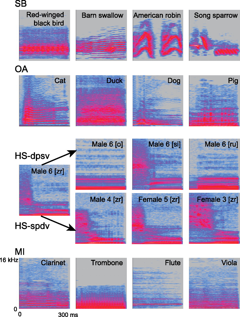
The four stimulus categories included songbirds (SBs), other animals (OAs), human speech (HS), and musical instruments (MIs) (Fig. 1). We established SBs as a separate category due to its spectrotemporal composition, which is distinct from OA sounds. Each category contained several subcategories (e.g., the animal category contained pig, cat, chicken, and additional animal species) (see supplemental Table 1, available at www.jneurosci.org as supplemental material). Subcategories were chosen such that it could be reasonably assumed that participants had heard these types of sounds directly from their respective sources (i.e., not just from recordings). Indeed, participants were able to accurately categorize individual stimuli after the scan (eight participants tested: mean accuracy, 94%; SD, 0.05), and performance did not differ across categories (one-way ANOVA: F(3,28) = 0.22, p = 0.88). Each subcategory was composed of 12 acoustically distinct tokens (e.g., 12 separate cat vocalizations). The human speech category contained 12 voices (6 male, 6 female) uttering 12 phoneme combinations ([bl], [e], [gi], [kae], [o], [ru], [si], [ta], [u], [zr]).

Example stimulus spectrograms for each category. Each row of four spectrograms represents an example trial. On each trial, four stimuli were presented, all from the same category (SBs, OAs, HS; HS-dvsp, HS-svdp, or MIs). Each stimulus was 300 ms in duration, as indicated by the length of the x-axis of the spectrograms. Frequency is plotted along the y-axis (0–16 kHz, linear scale), and stimulus intensity is denoted by color (grays and blues indicate low amplitude, pinks indicate high amplitude in dB).
Stimuli were 300 ms in duration, edited from high-quality “source” recordings taken from websites and compact discs (OAs, SBs, MI) or original recordings (HS). Cropping was done at zero crossings, or using short (5–10 ms) on- and off-ramps to prevent distortion. Source recordings were high quality (minimum: 44.1 kHz sampling rate; 32 kbit/s bit rate), with the exception of a small number of OA files (∼20%; 22.05 kHz sampling rate; 32 kbit/s bit rate). All stimuli were up- or down-sampled to a 44.1 kHz sampling rate and 32 kbit/s bit rate. Stimulus amplitude was then normalized such that the root mean square (rms) power of each stimulus was identical, which can be confirmed by noting the equal area under each power spectrum curve in Figure 2A. Though not identical with it, rms normalization is a common means of approximating perceived loudness across stimuli.

Acoustic features as a function of stimulus category. A, Mean power spectra are plotted for each stimulus category (SBs, red; OAs, orange; HS, green; MIs, blue; color scheme remains consistent throughout). Frequency is plotted in linear scale on the x-axis, while intensity is plotted on the y-axis. Mean power spectra are plotted again in the inset, with frequency shown in log scale along the x-axis, which better approximates the perceptual distances between frequencies in humans. B, Spectral content. FC (left) and pitch (right) are plotted in color for each stimulus; mean values are in black. y-axes are plotted in log scale. C, Temporal variability. FCSD values (left) and AMSD values (right) are plotted as in B. D, Spectral structure. HNR (left) and PS (right) are plotted as in B and C.
Stimulus acoustic features
All acoustic analyses were performed using Praat software (www.praat.org). Several acoustic features (Fig. 2) were assessed, including measures of spectral content, spectral structure, and temporal variability.
Spectral content.
The spectral content of each stimulus was assessed in two ways: spectral center of gravity and pitch. To calculate spectral center of gravity, Praat first performs a fast Fourier transform of the stimulus. It then calculates the mean frequency value of the resulting spectrum, weighted by the distribution of signal amplitudes across the entire spectrum. Thus, the resultant value reflects the center of gravity of the spectrum, an approximation of overall frequency content (FC).
Pitch was calculated using an autocorrelation method, adjusted to reflect human perceptual abilities (Boersma, 1993). This measure of temporal regularity (i.e., periodicity) corresponds to the perceived frequency content (i.e., pitch) of the stimulus. The autocorrelation method takes the strongest periodic component (i.e., the time lag at which a signal is most highly correlated with itself) of several time windows across the stimulus and averages them to yield a single mean pitch value for that stimulus. The size of the time windows over which these values are calculated in Praat are determined by the “pitch floor,” or the lowest frequency pitch candidate considered by the algorithm. We chose a default pitch floor of 60 Hz (resulting in 0.0125 s calculation windows); however, this value was lowered to 20 Hz for stimuli with fundamental frequencies <60 Hz.
Spectral structure.
Measures of stimulus spectral structure included pitch strength (PS) and harmonics-to-noise ratio (HNR). PS reflects the autocorrelation value of the strongest periodic component of the stimulus [i.e., r′(tmax)] using the method described above (Boersma, 1993). This measure thus reflects the perceived strength of the most periodic component of the stimulus, which is related to the salience of the pitch percept. Similarly, HNR measures the ratio of the strength of the periodic and aperiodic (i.e., noisy) components of a signal (Boersma, 1993). HNR is calculated in a single time window as follows:
 where r′(tmax) is the strength of the strongest periodic component and (1 − r′(tmax)) represents the strength of the aperiodic component of the signal. Thus, positive HNR values denote a periodic stimulus (high spectral structure), while negative values indicate a noisy stimulus (low spectral structure).
Temporal variability.
We assessed temporal variability using Praat in two separate stimulus dimensions: frequency and amplitude. The SD of FC values (FCSD) was determined by the distribution of power across the frequency spectrum (described above). Amplitude SD (AMSD) was the SD in stimulus energy calculated across the duration of the stimulus in time windows determined by the lowest estimated periodic frequency for that stimulus (i.e., pitch floor 60 Hz, or lower for select stimuli).
Stimulus presentation
During scans, stimuli were presented via in-ear electrostatic headphones (STAX), constructed to have a relatively flat frequency response up to 20 kHz (±4 dB). Stimuli were played at a comfortable volume (∼60–65 dB), with attenuation of ambient noise provided by ear defenders (∼26 dB reduction; Bilsom). Each trial contained four same-category stimuli separated by 150 ms interstimulus intervals (Fig. 1). Subcategories were not repeated within SB, OA, or MI trials. HS trials contained either (1) the same voice uttering four different phoneme combinations or (2) four different voices uttering the same phoneme combination. These two subtypes of HS trials were used to distinguish between brain areas responsive to human voice and speech sounds (see Repetition Adaptation). Care was taken that combinations of speech sounds within a trial did not create real words. The order of conditions across trials was pseudo-randomized (i.e., immediately adjacent condition repetitions were avoided). Trial types (Fig. 1) were presented 33 times each, divided across three runs, and included the following: silence; SB; OA; HS different acoustic–phonetic content same voice (HS-dpsv); HS same acoustic–phonetic content different voice (HS-spdv); and MI.
Participants performed an amplitude “oddball” task while in the scanner. On 3.3% of trials that were evenly distributed across stimulus categories, one of four stimuli was presented at a lower volume than the remaining three. Participants were instructed to indicate via separate button press whether the trial was an oddball or normal trial. Participants performed this task with relative accuracy (mean, 91.8%; SD, 3.7%; due to technical issues, behavioral data are missing for two subjects).
fMRI protocol and analysis
Images were acquired using a 3.0 tesla Siemens Trio scanner. Three sets of functional echo-planar images were acquired using a sparse sampling paradigm (repetition time, 8 s; acquisition time, 2.96 s; 33 axial slices; 3.2 × 3.2 × 2.8 mm3 resolution). A high-resolution anatomical scan (1 × 1 × 1 mm3) was also performed. All imaging analyses were completed using BrainVoyager QX (Brain Innovation). Functional images from each run were corrected for motion in six directions, corrected for linear trend, high-pass filtered at 3 Hz, and spatially smoothed using a 6 mm3 Gaussian filter. Data were then coregistered with anatomical images and interpolated into Talairach space (Talairach and Tournoux, 1988) at 3 × 3 × 3 mm3.
Random effects (RFx) group analyses using the general linear model (GLM) were executed across the entire brain and in regions of interest (ROIs) to assess the relationship between fMRI signal and our experimental manipulations (i.e., regressors) (Friston et al., 1995). RFx models were used to reduce the influence of intersubject variability (Petersson et al., 1999). Because we were only interested in auditory cortex, we restricted our analyses to voxels in temporal cortex that were significant for any category when compared with baseline. In these analyses, a single-voxel threshold of t(14) > 3.79, p < 0.005 was chosen; the resulting maps were then corrected for cluster volume at p(corr) < 0.05 using Monte Carlo simulations (a means of estimating the rate of false-positive voxels) (Forman et al., 1995). In ROI analyses, significance thresholds were corrected for multiple comparisons by using a Bonferroni adjustment for the number of post hoc contrasts performed in the relevant analysis. Following popular convention, whole-head statistical parametric maps were interpolated into 1 × 1 × 1 mm3 space for visualization in figures, but all analyses were performed in the “native” resolution of the functional data (3 × 3 × 3 mm3).
GLMs.
We used two types of GLMs in our analyses to assess the relationship between our conditions (i.e., regressors) and the dependent variable (i.e., fMRI signal) (Friston et al., 1995). In our “standard” model, the four conditions corresponding to stimulus categories (SB, OA, HS, and MI) and amplitude oddball trials were included as regressors. We used this model as an initial test of category selectivity. In a second “combined” model, we included additional regressors that reflected the mean values per trial of our chosen acoustic features. Thus, by entering both category conditions and mean acoustic feature values into the same GLM, we were able to assess category selectivity while “partialling out” (i.e., statistically controlling for) the influence of low-level acoustic features on the fMRI signal. Conversely, we also used the combined model to measure parametric sensitivity to our chosen acoustic features. Critically, acoustic feature values were z-normalized before being entered into the combined model, thus allowing examination of the parametric effect independent of baseline (i.e., independent of the main effect of auditory stimulation). Averaging acoustic feature values across four stimuli within a trial is perhaps less straightforward than “averaging” category information within a trial (or restricting trials to a single stimulus); however, the current four-stimulus paradigm affords a potential boost in overall fMRI signal and allows us to examine repetition adaptation effects in HS trials (see below).
GLMs with highly intercorrelated regressors can be inaccurate in assessing relationships between individual regressors and the dependent variable (i.e., multicollinearity). In our data, two spectral content features (FC and pitch) were highly intercorrelated (r = 0.85, p < 0.0001), as were the two measures of spectral structure (PS and HNR: r = 0.73, p < 0.0001). So, we adjusted the combined model to accommodate this issue.
A common way to address multicollinearity is to compare the outcomes of models that include one intercorrelated regressor while excluding the other, and vice versa. In our analyses, the results were nearly identical regardless of whether FC or pitch was included; thus, only those analyses including FC are discussed here. In regard to PS and HNR, we constructed two complementary GLMs. The first model omitted HNR and included the following regressors: FC, PS, FCSD, AMSD, SB, OA, HS, MI, and amplitude oddball trials. The second model omitted PS and included FC, HNR, FCSD, AMSD, SB, OA, HS, MI, and oddball trials. The outcomes of these two models were slightly different, so we present the results of both here. We used: (1) the first model to accurately assess the effects of PS and (2) the second model to assess the effects of HNR; while (3) significant results from both models were used to assess the effects of stimulus category, FC, FCSD, and AMSD.
Repetition adaptation.
The two subtypes of human speech trials (HS-svdp and HS-dvsp) were treated as the same regressor or “condition” for most analyses. In one exception, fMRI signal associated with these two human speech trial types was compared to identify voxels that respond differentially to human voice or to acoustic–phonetic content. To do this, we used the fMRI repetition adaptation phenomenon (Belin and Zatorre, 2003; Grill-Spector et al., 2006; Sawamura et al., 2006). Thus, those voxels that respond preferentially to human voice should exhibit fMRI signal adaptation (i.e., reduction in signal) to trials in which the same human voice was repeated across stimuli and a release from adaptation (i.e., increase in signal) in trials with different human voices. Conversely, voxels that respond preferentially to acoustic–phonetic content should exhibit adapted signal to trials with repeated phonemes compared with trials with different phonemes. This analysis used the combined model (see above), and its results were corrected for cluster volume at p(corr) < 0.001 (single-voxel threshold: t(14) > 2.62, p < 0.02).
Percent signal change calculation for charts.
For visualization in charts in figures, the percent signal change was calculated in reference to a statistically estimated “baseline.” In these calculations, baseline corresponded to the constant term estimated by the standard model (i.e., the value of fMRI signal estimated by the model, assuming all conditions/regressors were zero). This method is widely used and is comparable to other calculation methods (i.e., calculating the percentage signal change from the mean signal per run or during silent/baseline trials). Note that these calculations were used for visualization in figure charts only; statistical analyses were performed on the z-normalized single-voxel or ROI data, as per convention.
Results
Acoustic analysis of stimuli
The stimulus set included sounds from four different object categories: SB, OA, HS, and MI (Fig. 1). All stimulus categories were heterogeneous with respect to acoustic content (Fig. 2), although they were matched for duration and amplitude. We assessed several acoustic features, including two measures each of spectral content (FC and pitch), spectral structure (PS and HNR), and temporal variability (FCSD and AMSD). Statistical comparisons (multifactor ANOVA with post hoc pairwise comparisons using Tukey honestly significant difference tests) revealed the significant main effects of category for all six features (FC, F(3,448) = 273.96; pitch, F(3,448) = 222.943; PS, F(3,448) = 32.20; HNR, F(3,448) = 47.01; FCSD, F(3,448) = 17.74; AMSD, F(3,448) = 34.70; p < 0.001 for all). SB stimuli were significantly higher on measures of actual (FC) and perceived (pitch) spectral content than OA, MI, or HS categories (p < 0.001 for all) (Fig. 2B). MI stimuli had significantly stronger spectral structure (PS and HNR) than any other category (p < 0.001 for all) (Fig. 2D) but also exhibited lower temporal variability (FCSD, p < 0.001; AMSD, p < 0.01) (Fig. 2C). No other comparisons were significant. Some acoustic variability across categories is expected; perfect normalization of acoustic differences would result in a set of identical stimuli. Importantly, most distributions were large and overlapping across categories (Fig. 2B–D), justifying the use of these features as regressors in subsequent fMRI analyses (see further below).
Category-selective activity in auditory cortex
We defined “category-selective” voxels as those having fMRI signal for a single category that was greater than that for any other category. Thus, for example, “MI-selective” voxels were selected based on the statistically significant result of the conjunction of three pairwise contrasts: (1) MI > SB, (2) MI > OA, and (3) MI > HS. These analyses yielded several category-selective clusters within nonprimary auditory cortex (Fig. 3; supplemental Table 2A, available at www.jneurosci.org as supplemental material). HS-selective clusters were located bilaterally on the middle portions of superior temporal cortex (mSTC), including the superior temporal gyri and sulci (upper bank) of both hemispheres. Clearly separate from these HS-selective voxels were MI-selective clusters located bilaterally on lateral Heschl's gyrus (lHG). An additional MI-selective cluster was located in an anterior region of the right superior temporal plane (RaSTP), medial to the convexity of the superior temporal gyrus. No voxels were selective for either SB or OA stimuli. Voxels exhibiting no significant difference between any pair of stimulus categories (p(corr) > 0.05, Bonferroni correction for the number of voxels significantly active for every category) encompassed medial Heschl's gyrus (mHG), which is the most likely location of primary auditory cortex (Rademacher et al., 2001; Fullerton and Pandya, 2007), and adjacent areas of the posterior superior temporal plane (pSTP) or planum temporale (Fig. 3, white clusters).

Category-selective regions of auditory cortex. A, Group functional maps are overlaid on group-averaged anatomical images, rotated to visualize the superior temporal plane in oblique horizontal sections. Category-selective voxels are shown in color: green clusters indicate regions selectively responsive to human speech sounds; blue indicates clusters selective for musical instrument sounds. No voxels were selective for songbird or other animal sounds. Significant category-selective voxels reflect the results of independent conjunction analyses, identifying areas significantly greater for each category than each remaining category (p(corr) < 0.05). White voxels were significantly active for all four stimulus categories (t(14) > 3.79, p(uncorr) < 0.005) but demonstrated no significant differences between pairwise comparisons of category (p(corr) > 0.05). Sagittal sections are 10 mm apart within each hemisphere (top row). Oblique horizontal images (middle) are 7 mm apart and are arranged from inferior (left) to superior (right). Coronal sections (bottom) are 17 mm apart and arranged from posterior to anterior. B, Signal is plotted for representative functional voxels from clusters that exhibited no significant difference (n.s.) in response across categories (mHG, pSTP) and two category-selective clusters (speech, LmSTC; music, RaSTP).
This pattern of category-selective activation was also largely robust to cross-validation; testing two randomly selected halves of the dataset yielded similar patterns of activation (Table 1). However, the amount of overlap between voxels identified using each half of the dataset varied. For example, although both halves elicited MI-selective activation on lHG, each identified an independent selection of voxels (0% overlap). In RaSTP, on the other hand, 100% of voxels identified by half number 1 were significant when testing half number 2, indicating these voxels were indeed consistently MI selective. Similarly, HS-selective voxels in the left and right mSTC were robust to cross-validation, though a greater percentage of these voxels overlapped in the left hemisphere cluster than in the right. Thus, while lHG did not pass this assessment, RaSTP and bilateral mSTC remained category-selective in both halves of the dataset.
Talairach coordinates of category-selective clusters with cross-validation analysis
Relationship between acoustic features and category selectivity
Utilizing the acoustic heterogeneity of our stimulus set, we examined the extent to which a category-selective signal was influenced by our chosen spectral and temporal acoustic features. Thus, we identified category-selective voxels, using a combined analysis that measured the effects on fMRI signal of both category and the mean value of each acoustic feature per trial (see Materials and Methods). Using this combined analysis, we identified voxels that responded selectively to a particular category independent of the effect of stimulus acoustic features, and vice versa.
When accounting for the effect of acoustic features on fMRI signal, RaSTP and left mid superior temporal sulcus (LmSTS) remained MI and HS selective, respectively (RaSTP: X,Y,Z = 50, 1, 0; volume = 108 mm3; LmSTS: X,Y,Z = −60, −24, 3; volume = 1836 mm3) (Fig. 4). By contrast, lHG was no longer significantly MI selective, nor was right mSTC (RmSTC) selective for HS sounds.

Sensitivity to acoustic features in auditory cortex. Group functional maps from the standard (Fig. 3) and combined models are overlaid on anatomical images from a single representative subject, rotated to visualize STP. The combined model included both stimulus category and acoustic features (FC, PS, HNR, FCSD, and AMSD) as model regressors. Category-selective voxels from the standard model are shown in light green (HS) and light blue (HS). Remaining category-selective voxels identified with the combined model (i.e., after statistically controlling for the acoustic feature effects) are depicted in dark green (HS) and dark blue (MI) and encircled in white. Clusters exhibited significant relationships with acoustic features, including PS (pink), HNR (purple), and AMSD (yellow). The asterisk marks the cluster exhibiting a significant parametric relationship with AMSD in both combined models (see Materials and Methods) (supplemental Table 3, available at www.jneurosci.org as supplemental material). White voxels are marked as in Figure 3.
To assess whether any acoustic feature in particular influenced the “misidentification” of lHG and RmSTC as MI and HS selective, respectively (Fig. 3), we conducted an ROI analysis, applying the combined model to the mean signal in these clusters (supplemental Table 3, available at www.jneurosci.org as supplemental material). Left lHG was particularly sensitive to PS (p(corr) < 0.05, corrected for the number of tests performed), while a similar effect of PS in right lHG (RlHG) was less robust (p(corr) > 0.05, p(uncorr) < 0.006). Signal in RmSTC exhibited a modest negative relationship with AMSD (p(corr) > 0.05, p(uncorr) < 0.011), indicating perhaps a more complex relationship among category, acoustic features, and fMRI signal in this cluster. Neither category-selective ROI (RaSTP, LmSTS) demonstrated a significant relationship with any acoustic feature tested (supplemental Table 3, available at www.jneurosci.org as supplemental material).
This combined model also allowed us to identify several clusters along the STP that were particularly sensitive to acoustic features, when controlling the influence of stimulus category. Clusters located bilaterally along mid-STP, aSTP, and lHG exhibited a positive parametric relationship with PS (Fig. 4). An additional RaSTP cluster was sensitive to HNR as well (Fig. 4). None of these clusters sensitive to PS and HNR overlapped with MI-selective voxels in RaSTP at our chosen threshold. Additionally, bilateral regions of lateral mSTG were sensitive to AMSD (Fig. 4); however, only right hemisphere voxels were significant for this negative relationship in both analysis models (supplemental Table 3, available at www.jneurosci.org as supplemental material) (see Materials and Methods). No voxels exhibited significant sensitivity to FC or FCSD.
Heterogeneity in HS-selective areas
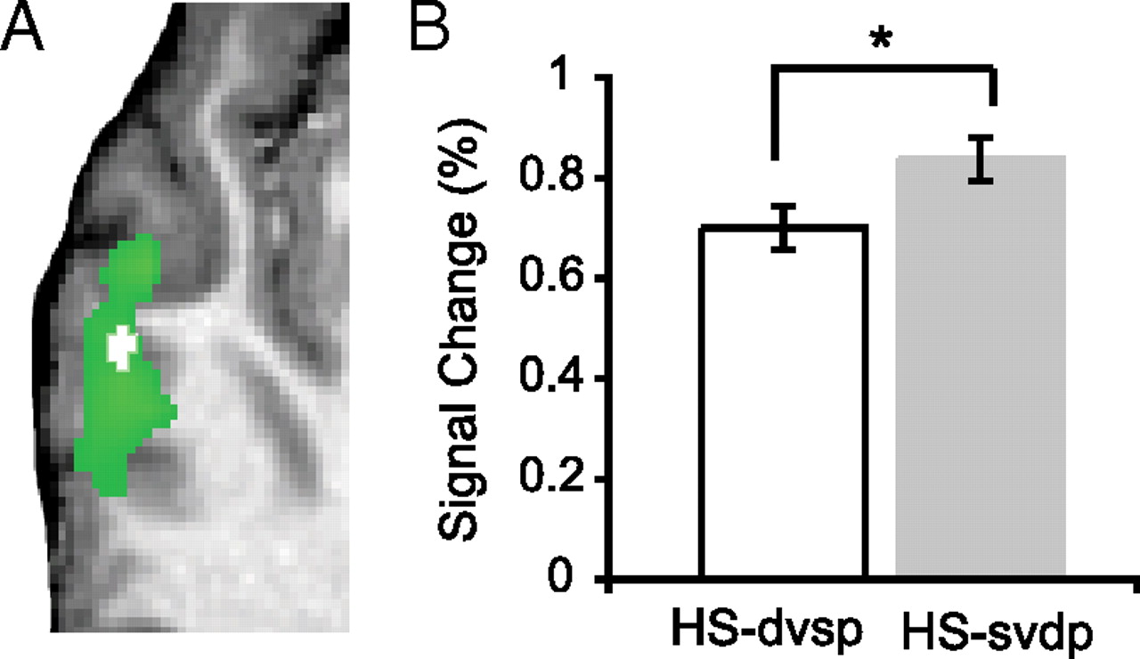
Within HS-selective voxels from the combined model described above, we identified LmSTS voxels that responded preferentially to the acoustic–phonetic content of speech trials. To do this, we compared fMRI signal associated with trials in which acoustic–phonetic content was varied but the speaker remained the same (HS-dpsv) (Fig. 1) and those trials in which acoustic–phonetic content was the same and the speaker varied (HS-spdv) (Belin and Zatorre, 2003). Evidence from fMRI repetition adaptation (fMRI-RA) suggests that voxels selective for the variable of interest (i.e., either acoustic–phonetic content or the speaker's voice) would exhibit increased signal (i.e., release from adaptation) to trials in which the content of interest was varied (Grill-Spector et al., 2006; Sawamura et al., 2006) (see Materials and Methods). If signal was equivalent across these trial types, then these voxels could be considered equally responsive to acoustic–phonetic content and the speaker's voice. An analysis restricted to HS-selective voxels identified a subregion of anterior LmSTS (X,Y,Z = −60, −20, 1; volume = 108 mm3) that had greater signal for HS-dpsv trials than HS-spdv trials (Fig. 5). Thus, this subregion can be considered selective for acoustic–phonetic content. The signal in all other voxels was not different across these speech trials (cluster corrected at p(corr) < 0.001; single-voxel threshold: t(14) > 2.62, p < 0.02).

Subregion of left superior temporal sulcus selective for acoustic–phonetic content of human speech sounds. A, A “masked” analysis restricted to regions identified as HS selective (green) demonstrated an anterior subregion of LmSTS (white) that was selective for the acoustic–phonetic content of human speech stimuli. The mask was defined (and subsequent analysis was performed) using the combined analysis with both trial category and acoustic features considered (p(corr) < 0.001; both models yielded similar results) (see Materials and Methods). Group data are overlaid on anatomical images from a representative single subject. B, The ROI in A was identified as phoneme selective using fMRI-RA; the signal associated with trials in which acoustic–phonetic content was the same (white) was significantly lower than that in trials in which acoustic–phonetic content was varied (gray). The mean ROI signal is depicted here for illustrative purposes only; asterisk indicates significance for voxelwise statistics in A. Error bars indicate SEM.
Discussion
By mitigating the potential influences of attention, semantics, and low-level features on fMRI responses to auditory objects, we functionally parcellated human auditory cortex based on differential sensitivity to categories and acoustic features. Spatially distinct, category-selective subregions were identified in anteroventral auditory cortex for musical instrument sounds, human speech, and acoustic–phonetic content. In contrast, regions relatively more posterior (i.e., closer to auditory core cortex) were primarily sensitive to low-level acoustic features and were not category selective. These results are suggestive of a hierarchically organized anteroventral pathway for auditory object processing (Griffiths et al., 1998; Rauschecker and Tian, 2000; Wessinger et al., 2001; Davis and Johnsrude, 2003; Lewis et al., 2009). Our data indicate that these intermediate stages in humans may be particularly sensitive to spectral structure and relatively lower rates of temporal modulation, corroborating the importance of these features in acoustic analysis (Zatorre et al., 2002; Boemio et al., 2005; Bendor and Wang, 2008; Lewis et al., 2009). Moreover, some of our tested stimulus categories seem to be processed in category-specific subregions of aSTC, which indicates that both distributed and modular representations may be involved in object recognition (Reddy and Kanwisher, 2006).
Auditory cortical responses to human speech sounds
Bilateral mSTC responded best to HS sounds. However, when controlling for the effects of acoustic features, only LmSTC remained selective for HS, while RmSTC responded equally to all categories. Additionally, anterior LmSTS was optimally sensitive to the acoustic–phonetic content of human speech, suggesting that this subregion may be involved in identifying phonemes or phoneme combinations.
Previous studies have implicated the STS in speech processing (Binder et al., 2000; Scott et al., 2000, 2006; Davis and Johnsrude, 2003; Narain et al., 2003; Thierry et al., 2003), with adaptation to whole words occurring 12–25 mm more anterior to the region we report here (Cohen et al., 2004; Buchsbaum and D'Esposito, 2009; Leff et al., 2009). Critically, because the present study used only single phonemes (vowels) or two-phoneme strings, the subregion we report is most likely involved in processing the acoustic–phonetic content, and not the semantic or lexical content, of human speech (Liebenthal et al., 2005; Obleser et al., 2007). Additionally, this area was invariant to speaker identity and naturally occurring low-level acoustic features present in human speech and other categories. Therefore, our anterior LmSTS region appears to be exclusively involved in representing the acoustic–phonetic content of speech, perhaps separate from a more anterior subregion encoding whole words.
A “voice-selective” region in anterior auditory cortex has been identified in both humans (Belin and Zatorre, 2003) and nonhuman primates (Petkov et al., 2008). Surprisingly, we did not find such a region using fMRI-RA. We suspect that the voices used in the present study may not have had sufficient variability for any measurable release from adaptation to voice: for example, our stimulus set included adults only, while Belin and Zatorre (2003) included adults and children. Given these and other results (Fecteau et al., 2004), we do not consider our results contradictory to the idea of a voice-selective region in auditory cortex.
Auditory cortical responses to musical instrument sounds
After accounting for the influence of low-level acoustic features, a subregion of RaSTP remained selective for MI sounds. Although MI stimuli are highly harmonic, MI-selective voxels did not overlap with neighboring voxels sensitive to PS and HNR. Also, our brief (300 ms) stimuli were unlikely to convey complex musical information like melody, rhythm, or emotion. Thus, RaSTP seems to respond preferentially to musical instrument sounds.
Bilateral aSTP has been shown to be sensitive to fine manipulations of spectral envelopes (Overath et al., 2008; Schönwiesner and Zatorre, 2009), while studies using coarse manipulations generally report hemispheric (vs regional) tendencies (Schönwiesner et al., 2005; Obleser et al., 2008; Warrier et al., 2009). Thus, aSTP as a whole may encode fine spectral envelopes, while MI-selective RaSTP could encode instrument timbre, an aspect of which is conveyed by fine variations of spectral envelope shape (Grey, 1977; McAdams and Cunible, 1992; Warren et al., 2005). However, alternative explanations of RaSTP function should be explored (e.g., aspects of pitch/spectral perception not captured by the present study), and further research is certainly needed on this underrepresented topic (Deike et al., 2004; Halpern et al., 2004).
Sensitivity to spectral and temporal features in auditory cortex
Auditory cortex has been proposed to represent acoustic signals over temporal windows of different sizes (Boemio et al., 2005; Bendor and Wang, 2008), with a corresponding tradeoff in spectral resolution occurring within (Bendor and Wang, 2008) and/or between (Zatorre et al., 2002) hemispheres. Indeed, left auditory cortex (LAC) is sensitive to relatively higher rates of acoustic change than right auditory cortex (RAC) (Zatorre and Belin, 2001; Boemio et al., 2005; Schönwiesner et al., 2005), and this temporal fidelity is argued to be the basis of LAC preference for language (Zatorre et al., 2002; Tallal and Gaab, 2006; Hickok and Poeppel, 2007). Correspondingly, RAC is more sensitive to spectral information within a range important for music perception (Zatorre and Belin, 2001; Schönwiesner et al., 2005). Although we do not show sensitivity to high temporal rates in LAC, our data do indicate relatively greater spectral fidelity in RAC, with corresponding preference for slower temporal rates. Thus, our study corroborates the idea of spectral–temporal tradeoff in acoustic processing in auditory cortex, with particular emphasis on the importance of stimulus periodicity.
The perception of pitch arises from the analysis of periodicity (or temporal regularity) in sound, which our study and others have shown to involve lHG in humans (Griffiths et al., 1998; Patterson et al., 2002; Penagos et al., 2004; Schneider et al., 2005) and a homologous area in nonhuman primates (Bendor and Wang, 2005, 2006). Other clusters along the STP were sensitive to spectral structure in our study as well, and while the majority of these were sensitive to PS, one anterior subregion was sensitive to HNR, which has a nonlinear relationship to periodicity (Boersma, 1993). This suggests that not only are multiple subregions responsive to periodicity, but these subregions may process periodicity differently (Hall and Plack, 2007, 2009), which is compatible with studies reporting other regions responsive to aspects of pitch (Pantev et al., 1989; Langner et al., 1997; Lewis et al., 2009).
The nature of object representations in auditory cortex
Our data suggest that some types of objects are encoded in category-specific subregions of anteroventral auditory cortex, including musical instrument and human speech sounds. However, no such category-selective regions were identified for songbird or other animal vocalizations. This could be explained by two (not mutually exclusive) hypotheses. First, clusters of animal- or songbird-selective neurons could be interdigitated among neurons in regions selective for other categories or may be grouped in clusters too small to resolve within the constraints of the current methods (Schwarzlose et al., 2005). Future research using techniques that are better able to probe specificity at the neural level, such as fMRI-RA or single-cell recordings in nonhuman animals, will be better able to address these issues.
Alternatively, object recognition may not require segregated category-specific cortical subregions in all cases or for all types of objects (Grill-Spector et al., 2001; Downing et al., 2006; Reddy and Kanwisher, 2006). Instead, coincident activation of intermediate regions within the anteroventral pathway may be sufficient for processing songbird and other animal vocalizations. Such “category-general” processing of acoustic object feature combinations may involve regions like those responsive to coarse spectral shape or spectrotemporal distinctiveness in artificial stimuli (Rauschecker and Tian, 2004; Tian and Rauschecker, 2004; Zatorre et al., 2004; Warren et al., 2005), perhaps analogous to lateral occipital regions in the visual system (Malach et al., 1995; Grill-Spector et al., 2001; Kourtzi and Kanwisher, 2001). While such forms of neural representation might be considered “distributed” (Staeren et al., 2009), the overall structure remains hierarchical: neural representations of auditory objects, whether distributed or within category-specific subregions, depend on coordinated input from lower order feature-selective neurons and are shaped by the evolutionary and/or experiential demands associated with each object category.
Thus, our data are consistent with a hierarchically organized object-processing pathway along anteroventral auditory cortex (Belin et al., 2000; Scott et al., 2000; Tian et al., 2001; Poremba et al., 2004; Zatorre et al., 2004; Petkov et al., 2008). In contrast, posterior STC responded equally to our chosen categories and acoustic features, consistent with its proposed role in a relatively object-insensitive posterodorsal pathway (Rauschecker and Scott, 2009). Posterior auditory cortex has been shown to respond to action sounds (Lewis et al., 2005; Engel et al., 2009), the spatial properties of sound sources (Tian et al., 2001; Ahveninen et al., 2006), and the segregation of a specific sound source from a noisy acoustic environment (Griffiths and Warren, 2002). Future research furthering our understanding of how these pathways interact will offer a more complete understanding of auditory object perception.
Footnotes
- Received January 19, 2010.
- Revision received April 14, 2010.
- Accepted April 21, 2010.
-
This work was funded by the National Institutes of Health (Grants R01-NS052494 and F31-DC008921 to J.P.R. and A.M.L., respectively) and by the Cognitive Neuroscience Initiative of the National Science Foundation (Grant BCS-0519127 to J.P.R.).
- Correspondence should be addressed to Amber M. Leaver, 3970 Reservoir Road NW, Georgetown University Medical Center, Washington, DC 20057. aml45{at}georgetown.edu
- Copyright © 2010 the authors 0270-6474/10/307604-09$15.00/0