
Abstract
The retinotopic organization of macaque occipitotemporal cortex rostral to area V4 and caudorostral to the recently described middle temporal (MT) cluster of the monkey (Kolster et al., 2009) is not well established. The proposed number of areas within this region varies from one to four, underscoring the ambiguity concerning the functional organization in this region of extrastriate cortex. We used phase-encoded retinotopic functional MRI mapping methods to reveal the functional topography of this cortical domain. Polar-angle maps showed one complete hemifield representation bordering area V4 anteriorly, split into dorsal and ventral counterparts corresponding to the lower and upper visual field quadrants, respectively. The location of this hemifield representation corresponds to area V4A. More rostroventrally, we identified three other complete hemifield representations. Two of these correspond to the dorsal and the ventral posterior inferotemporal areas (PITd and PITv, respectively) as identified in the Felleman and Van Essen (1991) scheme. The third representation has been tentatively named dorsal occipitotemporal area (OTd). Areas V4A, PITd, PITv, and OTd share a central visual field representation, similar to the areas constituting the MT cluster. Furthermore, they vary widely in size and represent the complete contralateral visual field. Functionally, these four areas show little motion sensitivity, unlike those of the MT cluster, and two of them, OTd and PITd, displayed pronounced two-dimensional shape sensitivity. In general, these results suggest that retinotopically organized tissue extends farther into rostral occipitotemporal cortex of the monkey than generally assumed.
- extrastriate cortex
- function
- homology
- human
- monkey
- retinotopy
Introduction
Functional MRI (fMRI) is a powerful tool for investigating the retinotopic organization of macaque visual cortex in individual subjects (Brewer et al., 2002; Vanduffel et al., 2002b; Fize et al., 2003; Kolster et al., 2009; Patel et al., 2010; Arcaro et al., 2011). Using phase-encoding techniques, Kolster et al. (2009) were able to determine the cluster organization of the middle temporal area (MT) and its satellites. In addition, these authors described an additional hemifield ventral to the fundus superior temporal sulcus area (FST; Fig. 1A). They proposed that this hemifield representation corresponds to the dorsal posterior inferotemporal area (PITd) as described by Felleman and Van Essen (1991) (Fig. 1B) overlapping, at least partially, with the architectonically-temporal occipital area (TEO). This schema contradicts the proposed retinotopic organization of TEO as a single hemifield (Fig. 1C) described by Boussaoud et al. (1991). However, in later publications Ungerleider et al. (2008) suggest an additional region dorsal to TEO (Fig. 1D, ?). The features of area PITd described by Kolster et al. (2009) indicate that additional areas should lie between V4 and PITd, since the anterior border of V4 represents the horizontal meridian (HM; Fig. 1, blue) while the posterior border of PITd is a vertical meridian (VM; Fig. 1A, red line). Although Felleman and Van Essen (1991) located the ventral occipitotemporal area (VOT; Fig. 1B) in that vicinity, the retinotopic organization of the entire region anterior to V4 remained unclear.

Review of previous proposals (indicated by labels) for the retinotopic organization of cortical areas on the posterior inferotemporal gyrus. Blue dotted lines indicate the representations of the HM corresponding to the anterior border of V4. Red lines in A represent upper (dashed) and lower (solid) VM of PITd. Green lines in E and F indicate the representations of the lower (solid) and upper (dashed) VM, the anterior border of area V4A. The purple line in A represents the eccentricity ridge surrounding the MT cluster. A, Kolster et al., 2009; Kolster et al., 2010. Reproduced by permission of the Journal of Neuroscience. B, Felleman and Van Essen, 1991; reproduced by permission of Oxford University Press. C, Boussaoud et al., 1991; reproduced by permission of John Wiley & Sons. D, Ungerleider et al., 2008; reproduced by permission of Oxford University Press. E, Pigarev et al., 2002; reproduced by permission of Springer. F, G, Stepniewska et al., 2005; reproduced by permission of Oxford University Press.
In his initial description of V4, Zeki (1971b) suggested that V4 was flanked by a more rostral area, V4A, which was located dorsally in the prelunate gyrus and ventrally at the posterior part of the inferior occipital sulcus (IOS). It has a split hemifield representation, as do early visual areas V2, V3, and V4 (Fig. 1F). Subsequent studies confirmed the heterogeneity of single-cell properties in this region (Maguire and Baizer, 1984; Tanaka et al., 1986), but the nature of V4A remained unresolved. Subsequently, Gattass et al. (1988) and Boussaoud et al. (1991) proposed that V4, with the HM as anterior border, directly neighbors the TEO (Fig. 1C). A decade later, however, the original notion of an intervening area V4A revived in both physiological and anatomical studies. Pigarev et al. (2002) mapped an HM on the prelunate gyrus and a VM in the posterior bank of superior temporal sulcus (STS) representing the borders of V4A (Fig. 1E). In their study of the cortical connections of V4, Stepniewska et al. (2005) also depicted V4A as a split representation, distinct from the TEO (Fig. 1G).
In summary, considerable dispute remains concerning the retinotopic organization in cortex rostral to V4. The number of areas occupying this region ranges from one—TEO (Boussaoud et al., 1991)—to as many as four—VOT (Felleman and Van Essen, 1991), PITd, ventral posterior inferotemporal area (PITv), and V4A (Pigarev et al., 2002; Stepniewska et al., 2005). The aim of the present study was to apply detailed phase-encoding, high-resolution fMRI mapping (Engel et al., 1994; Sereno et al., 1995) to this extrastriate region to determine its retinotopic organization, should it exist.
Materials and Methods
Experimental design
The goal of this study is to map the topographic organization of the occipitotemporal cortex, a region anterior to area V4 and ventral to the MT cluster. Previous studies suggested ≥1 hemifield representation in this region, which would correspond to a transition from a split quarter field to a hemifield organization. Because potentially more areas with different functions exist in this region, retinotopic mapping alone might be insufficient to reach a firm conclusion about the detailed topographic organization. Therefore, we first performed a retinotopic mapping experiment to find evidence for field maps in this region, such as meridian and quarter field representations. In a second step, we performed functional tests to characterize the individual retinotopic units (quarter fields), thereby reducing the number of possible interpretations of the observed topographic organization. As the occipitotemporal cortex and neighboring regions are involved in motion and shape processing, we used motion and two-dimensional (2D) shape stimuli in the latter tests. In a third step, a functional grid analysis was performed based on the topographic organization, which enabled a high-resolution group analysis across all subjects even for strongly distorted cortical regions. This approach also enabled a direct comparison with a recent human retinotopic mapping study (Kolster et al., 2010). Additional characteristics of the visual areas, such as the population receptive field (pRF) sizes, were derived from the data to obtain objective criteria for ranking the areas in the monkey–human comparison (see below). Finally, the response amplitudes and cortical magnification factors of individual areas were extracted from the retinotopic data and used as a data quality measure as well as to establish a reference for comparison with previous and future studies.
Subjects
Three juvenile male rhesus monkeys (M1, M2, and M3; Macaca mulatta; 3–5 kg; 3–5 years of age) participated in the experiments. The animals were different from those used in the Kolster et al. study (2009). All animal care and experimental procedures met national and European guidelines and were approved by the ethical committee of the Katholieke Universiteit Leuven. The details of the surgical procedures, training of monkeys, and eye monitoring have been described previously (Vanduffel et al., 2002b; Fize et al., 2003; Ekstrom et al., 2008) and will be reviewed here only briefly.
MR scanning
Anatomical MRI acquisition.
High-resolution, T1-weighted anatomical images were collected on a 3 tesla full-body scanner (TIM Trio, Siemens) and used for segmentation, registration, and displaying of the functional results. Under ketamine-xylazine anesthesia, a magnetization-prepared rapid-acquisition gradient echo sequence with 208 sagittal slices, 320 × 260 in-plane matrix, and 0.4 mm isotropic voxels was used. Additional sequence parameters were set for M1 and M2 as follows: repetition time (TR), 2.2 s; echo time (TE), 2.52 ms; inversion time (TI), 900 ms; flip angle (α), 9°. The following parameters were used for M3 and resulted in significantly better gray-to-white-matter contrast (Fig. 2): TR, 2.7 s; TE, 3.35 ms; TI, 850 ms; α, 9°. Between 12 and 16 whole-brain volumes were acquired in a single session and averaged to improve the signal-to-noise ratio. A radial transmit–receive surface coil was used for M1 and M2 and a radial receive-only surface coil was used for M3 (both coils were 12 cm in diameter).

Functional volume and activation relative to anatomical volume in monkey M3. A, B, Horizontal and coronal T1-weighted images (MPRAGE), with lines indicate the gray–white border (yellow) and pial (red) surface. C, D, Horizontal and coronal T2*-weighted images (gradient echo EPI, average across a single run) with lines indicating the gray–white border (yellow) and pial (red) surface. E, F, Same as C and D but with functional overlay representing the response amplitude in the retinotopic experiments above a threshold of 0.75% signal change as indicated in by the first harmonic of the Fourier spectrum (Fig. 17). Dark blue and cyan dots indicate the node point of the white-matter and pial surfaces, respectively. The white arrows point to the location of the inferotemporal gyrus.
fMRI acquisition.
Functional images were acquired with a 3 T full-body scanner (TIM Trio, Siemens), using a gradient-echo T2*-weighted echo-planar imaging sequence (40 horizontal slices; TR, 2 s) with 19 ms TE and 1.0 mm isotropic voxels in the retinotopic experiments, and 17 ms TE and 1.25 mm isotropic voxels in the functional localizer experiments. The functional data were collected using a custom-built radial transmit coil and an eight-channel phased-array receive coil. Data were taken as accelerated images in generalized autocalibrating partially parallel acquisition mode with foot–head acceleration direction and an acceleration factor (integrated parallel acquisition technique) of 3. The resulting echo planar image (EPI) raw data were exported from the scanner and reconstructed using an offline SENSE reconstruction (sensitivity encoding; Pruessmann et al. (1999)) written in Matlab (Kolster et al., 2009). The reconstruction code was extended for the purpose of the present experiments by introducing a regularization least-square algorithm. Reference data were collected as proton-density-weighted images using a gradient refocused echo (GRE) sequence with the following parameters: TE, 4 ms; TR, 40 ms; α, 9°. The data were then fitted by third-order polynomials to create complex sensitivity maps for the SENSE reconstruction.
Contrast agent.
Before each scanning session, a contrast agent, monocrystalline iron oxide nanoparticle (MION; Sinerem, Laboratoire Guerbet), was injected into the monkey's femoral/saphenous vein (9–11 mg/kg). Use of the contrast agent improved the contrast/noise ratio by ∼3-fold (Vanduffel et al., 2001; Leite et al., 2002) and enhanced spatial selectivity of the MR signal changes (Zhao et al., 2005), compared with blood oxygenation level-dependent (BOLD) measurements. While brain activations produce increased MR signals in BOLD measurements, they led to decreased signals using MION, which is essentially a cerebral blood volume (CBV) measurement. Therefore, to improve the comparison between BOLD and CBV results, we inverted the polarity of the CBV signal-change values.
Visual stimuli
Stimulus presentation.
The subjects sat in a sphinx position inside a plastic monkey chair directly facing a display screen. During training and scanning, they were required to maintain fixation within a 2 × 2° window centered on a red dot (0.35 × 0.35°) in the middle of this screen during stimulus presentation. Eye positions were monitored at 120 Hz via pupil position and corneal reflection (Iscan). The monkeys were rewarded (fruit juice) for fixating the small red dot within the fixation window for long periods of time equal to a run duration. During fixation, the interval between consecutive rewards gradually decreased to motivate the animals to fixate for long, uninterrupted periods. Only the data obtained while the monkey maintained its gaze within the window >95% of the scan duration were finally used in the analysis.
Retinotopic mapping.
During retinotopic mapping sessions, we alternated between polar-angle and eccentricity runs, in which the retinotopic stimuli were presented as rotating wedges and expanding rings, respectively. Each run consisted of 128 measurements with a TR of 2 s resulting in a total duration of 256 s per run. Four cycles of rotating or expanding stimuli, each 64 s in duration, were presented per run. The lag of the hemodynamic response results in a delay of the cortical activations in the time domain, thereby creating a shift of the traveling-wave response to later time points. Thus activations induced by the stimulus at the end of a cycle will carry over to the beginning of the following cycle. To avoid a gap in the traveling-wave response at the beginning of the first of four cycles, the 8 s preceding each run was used to precondition the cortical responses by presenting the last four stimuli from the previous cycle. Using this procedure, the start of each of the four cycles was visually identical, which reduces potential errors in the phase measurements. Only stimuli turning clockwise were used, to avoid a superposition of responses from opposite stimulus directions, ensuring that activation returned to baseline between two consecutive cycles (for calibration see below).
The stimuli consisted of clockwise-rotating wedges and expanding annuli composed of segments that resembled checkerboard patterns, with the sides of the segments aligned in the radial direction. They were presented monochromatically with a black–white counter-phasing flicker frequency of 2 Hz on a gray background at a luminance equal to the average of the black and white segments. The sizes and rates of progression of both the wedge stimuli in the azimuthal direction and the annulus stimuli in the radial direction were designed with a constant duty cycle. Each point of the visual field was stimulated for 8 s during each cycle to maximize the hemodynamic response amplitude. A cycle duration of 64 s (Sereno et al., 1995), corresponding to a duty cycle of 12.5%, was chosen to separate the response peaks in time and to allow a return to baseline activation between stimulations in consecutive cycles. Except for the initial and final eccentricity values (see below), the stimulus design and timing was the same as that used in our earlier publications concerning macaque (Kolster et al., 2009) and human (Kolster et al., 2010) visual cortex.
Polar-angle measurements.
The polar-angle stimulus consisted of a rotating wedge spanning 45° in polar angle and 0.25–12.25° in eccentricity (Fig. 3A). The wedge was composed of four segments in the azimuthal direction and 24 segments radially. The aspect ratio of the segments was kept at ∼1:1 over the entire range of eccentricities by adjusting the radial sizes of the segments according to a log(r) law to approximate the human cortical magnification factor. The wedge was presented for 2 s (1 TR) at each of 32 equally spaced positions and advanced every TR by one segment in the azimuthal direction at an average rate of 0.0982 radian/s.

Visual stimuli and analytical methods. A, Visual stimuli used in this study: (a) rotating wedges and expanding rings used to map polar angle and eccentricity, respectively; (b) moving and static dot pattern used to identify regions of motion sensitivity in the cortex (the dots moved in 8 different directions along the two cardinal axes and the diagonals, alternating between forward and backward motion); (c) intact (left) and scrambled (right) 2D gray scale (top) and line shapes (bottom) used to identify regions of 2D shape sensitivity in the cortex. B, Schematic describing the effect of small (top left) compared with large (bottom left) pRF sizes on the response amplitudes measured in a retinotopic traveling-wave experiment. The resulting response amplitudes for small pRFs are narrow (top middle), while the ones for large pRFs are wide (bottom middle). The Fourier transform of the response amplitude (middle), which is a cyclic function of length N with four identical functions g placed at equidistant positions, is represented by a harmonic spectrum (right) consisting of non-zero amplitudes at each fourth harmonic frequency from 0 to ± N/2. Its envelope G is represented by a function that is equal to the Fourier transform of g. The FWHM of the envelope G is proportional to the reciprocal of the FWHM of the associated response amplitudes and therefore wide for small pRFs (top right) and narrow for large pRFs (bottom right). C, Schematic of the different steps of the functional grid analysis. Responses to functional test stimuli and retinotopic reference space (a) are associated through their location in cortex in the individual subjects. The red spot in each map denotes the same functional location in cortex at a given combination of eccentricity and polar angle of the same visual area, but can appear at different anatomical locations in different subjects (b). Using the retinotopic data as a reference, the functional responses in different subjects can be matched on a normalized reference grid (c). This grid allows for binning of the data according to the stimulus size independent of the individual anatomy (d). It does not require smoothing of the data and achieves group results on the scale of the spatial resolution of the EPIs.
Eccentricity measurements.
The eccentricity stimulus consisted of expanding annuli centered on the fixation point (Fig. 3A). These annuli consisted of two concentric rings of 24 squares in the azimuthal direction. Each annulus was presented stepwise for 2 s (1 TR) at one of the 31 radial positions. As with the polar stimulus, the aspect ratios of the squares contained in the annuli were kept at ∼1:1 over the entire range of eccentricities by adjusting the radial size according to a log(r) law to approximate the human cortical magnification factor. Consequently, the diameters and widths of the annuli as well as their radial positions also increased in size according to the log(r) law. The stimuli were masked at eccentricities <0.25° and >12.25°. The position of the first stimulus was chosen such that only the outside quarter of the annulus was visible during the first 2 s period (first TR) in the cycle. Correspondingly, the position of the penultimate stimulus was chosen such that only the inside quarter of the annulus was visible. During the last 2 s period (the 32nd TR) in the sequence, no annulus was shown. This was done to phase the annuli in and out slowly and to avoid sudden jumps from peripheral to central positions.
Motion sensitivity.
To localize the motion-sensitive areas, two runs were acquired in which a moving random texture pattern 7° in diameter (50% high contrast, white dots 5 minarc in size) alternated with the same static pattern (Sunaert et al., 1999).
Two-dimensional shape sensitivity.
The standard 2D shape localizer (Malach et al., 1995; Kourtzi and Kanwisher, 2000; Denys et al., 2004) included four conditions: grayscale images or line drawings of familiar and unfamiliar objects, as well as scrambled versions of each set. These images were presented behind a 12 × 12° grid, the object images themselves averaged 9–10° in diameter.
The motion and shape stimuli used here were identical to the stimuli used in Kolster et al. (2010).
Imaging data processing
Data acquisition.
A total of 66,572 functional volumes were acquired in nine experiments: 32,384 volumes in three subjects for the retinotopic experiments (M1, 14,080 volumes in four sessions; M2, 10,880 volumes in three sessions; M3, 7424 volumes in two sessions), 16,632 volumes in three subjects for the motion localizer (M1, 7524 volumes; M2, 5742 volumes; M3, 3366 volumes; each representing a single session), and 17,556 volumes in three subjects for the 2D shape localizer (M1, 6156 volumes; M2, 6384 volumes; M3, 5016 volumes; each within a single session). To analyze these data, retinotopic and functional data from a given animal acquired in different sessions had to be aligned.
Image alignment.
Image alignment was carried out on two levels. First, a local correction was applied to each EPI image, which accounts for the dynamic differences between images within a session, mostly due to body motion. This is followed by a second, global correction, which accounts for static differences between the sessions due to differences in B0 shimming and positioning inside the scanner. For this purpose, a custom motion-correction was employed (Kolster et al., 2009) to correct the raw EPI images with respect to an EPI reference image chosen from the same session. The algorithm uses ≤3 parameters for zero-order to second-order polynomials to model shifts and distortions in the phase-encoding (PE) direction and ≤3 parameters for modulations of the above functions in frequency-encoding (FE) direction. Typically, a total of four parameters, either two in the PE direction and two in the FE direction or three in the PE direction and one in the FE direction, were sufficient to align the images. The correction was applied as a 2D distortion field of the grid points in the horizontal EPI images and the corrected image values were calculated by interpolation based on the initial image values and the distortion field. Each slice was corrected independently based on the target EPI volume, which was selected from a run within the same session after visual inspection to avoid slanted positions of the odd and even slices. Next, a global correction was applied, in which the GRE reference volumes of each session were aligned to the T1 volumes using a rigid-body, six-parameter alignment tool (www.nitrc.org/projects/jip; Mandeville et al., 2011). The resulting alignment was applied to the EPI volumes, as these are intrinsically aligned to the GRE volumes. Session-averaged EPI volumes were then registered to the T1 volumes using 2D distortion fields in the horizontal imaging plane (www.nitrc.org/projects/jip). Alignment between subsequent sessions was performed by registration of the GRE volumes of the additional sessions to the GRE volume of the reference session using a six-parameter rigid-body alignment and applying these registrations to the respective EPI volumes of the additional sessions. The EPI volumes were then further registered to the reference EPI volume by the use of 2D distortion fields in the horizontal imaging plane and aligned to the T1 volume using the EPI-to-T1 registration results of the reference session (Fig. 2).
Data analysis.
Segmentation of the anatomical volumes was carried out using Freesurfer (Fischl et al., 1999; http://surfer.nmr.mgh.harvard.edu), and inflated as well as flattened surface representations were created for each subject. The retinotopic measurements were analyzed in Freesurfer and further processed in Matlab (Mathworks). Analyses of the functional localizer measurements were carried out using jip-glm (www.nitrc.org/projects/jip) and visualized on the flat maps in Freesurfer.
Node-based analysis.
The surface representation of an individual cortical hemisphere as created in Freesurfer consists of a fine mesh of vertex points, also referred to as nodes, that are created during segmentation and that represent three-dimensional (3D) coordinates on the 2D surface separating white from gray matter (the “white-matter surface”). Each node is further associated with a fixed point on the pial surface through the direction and length of the normal vector originating at the node. Data were analyzed by aligning the functional data volumes to the anatomical volume, then projecting the data values found in voxels that correspond to locations in the gray-matter volume onto the nodes on the white-matter surface. This is done by selecting points along the normal vector of a particular node, assigning the local voxel values to these points, and defining an algorithm for this set of points, the result of which is then associated with the node. The number of voxels contributing to a node value will vary, depending on the local orientation and thickness of the gray matter. Nodes are further grouped under labels, which represent a subset of nodes associated with a common characteristic, e.g., a specific visual area. All further analysis of the retinotopic data is carried out using these node values, a strategy that restricts the analysis to data predominantly associated with gray matter. The nodes are also used to define a relationship between the sets of data from the retinotopic and functional test experiments, which are acquired at different resolutions and use different algorithms to compute the values associated with the nodes.
Retinotopic analysis
Analysis of retinotopic data.
All runs of the eccentricity or polar-angle experiments acquired across all sessions for a given monkey were averaged into single data volumes 128 time points in length. No temporal and spatial smoothing was applied to the data, apart from the smoothing inherent to registering and averaging functional volumes. The time course for each voxel was then analyzed for amplitude and phase using Freesurfer tools. The phase information, which is related to the delay of the local hemodynamic response with respect to the start of the run, was extracted and projected onto the nodes. To that end, three points along the normal vectors at 25, 50, and 75% of the local gray-matter thickness were defined and an average phase value of the voxels overlapping these points was assigned to each node. The upper and lower limits associated with these points require a minimum overlap with the gray-matter volume for the voxels contributing to each node. Averaging over multiple points along the normal vector at distances of ∼0.3 times the voxel size (assuming an average gray-matter thickness of 2 mm) results in an effective weighting function that assigns a greater weight to those voxels showing more overlap with gray matter. The data were then further smoothed on the surface performing a single iteration of the nearest-neighbor smoothing algorithm in Freesurfer. The resulting values for phase and amplitude associated with each node were stored for further analysis. The following analyses were restricted to nodes for which the amplitude at the cycle frequency, as returned by the Freesurfer tool, exceeded a threshold of 0.75. Figure 2E,F shows plots of the average aligned EPI volumes from monkey M3 with overlays of the node points from the main and pial surfaces as well as the functional overlays of the response amplitudes from the retinotopic analysis thresholded at 0.75% signal change of the CBV signal. White arrows mark the positions of the posterior inferotemporal gyrus in each hemisphere. The activations are clearly confined to the space between the main and pial surfaces indicating good overall alignment of the functional (Fig. 2C,D) and anatomical (Fig. 2A,B) volumes.
Significance and calibration of the retinotopic measurements.
The average magnitudes of the Fourier components corresponding to the cycle frequency (4 cycles/256 s) and its harmonics were computed for the eccentricity and polar-angle experiments and analyzed for significance in the following steps. The time course of each voxel was first Fourier transformed and the amplitudes saved as 128 volumes, one volume for each spectral component. These volumes were projected onto the surfaces nodes of individual subjects using the same algorithm as for the phase values. The average magnitudes were next computed for all nodes within each cortical area of a single hemisphere for eccentricities between 0.25 and 6.25°. Within this range, sufficient data points were available to compute a meaningful average for each area in each hemisphere of each monkey, including these areas with limited peripheral eccentricity representations. The average of all Fourier components not associated with the cycle frequency or one of its harmonics represents a 1/f noise spectrum and was used to interpolate the noise level at the cycle frequency and its harmonics in a procedure similar to that of Swisher et al. (2007). The resulting noise spectrum was then subtracted from the eccentricity and polar-angle spectra of each hemisphere. Finally, the resulting noise-corrected data were used to calculate, for a given cortical area and each harmonic frequency, the mean magnitude, the SE, and the t statistics across six hemispheres, for polar-angle and eccentricity data separately. To estimate the lag in the hemodynamic response and to calibrate the phase values for polar angle and eccentricity, the data were plotted onto a coordinate system representing the visual field. A phase correction for the polar angle was determined by visually inspecting the deviation from a vertical orientation of the line separating the data of the left and right hemispheres. The correction factors applied were set equal for polar angle and eccentricity. The correction was further confirmed by correlating the eccentricity data with the motion responses in area V1 (see functional grid analysis below). Due to the cyclical nature of the eccentricity angle, a phase shift in the eccentricity can displace data either from peripheral to central values or vice versa. Since the V1 responses to the motion paradigm are positive at central eccentricities and the peripheral responses negative (see text) a clear distinction can be made between central and peripheral data. An incorrect phase shift calibration will lead to an obviously erroneous assignment of positive values to peripheral eccentricities or negative values to central eccentricities.
Retinotopic maps.
Identification of the visual areas V1–V4 and the areas within the MT cluster can be carried out using the field-sign map as described in Sereno et al. (1995). To obtain the field-map representations of the occipitotemporal areas, we analyzed the retinotopic organization of these regions as follows. First, the central representations were identified for each area. Iso-polar-angle lines (Arcaro et al., 2009, 2011) were then drawn radially from the central representation outwards along the lines of constant polar angle associated with the HM and VM representations. The positions of the lines were determined by optimizing the color contrast and the brightness of the maps until the representations of VMs (maxima and minima) and HMs (transition between maxima and minima) were visible. Additional iso-polar-angle lines were drawn for intermediate polar angles between the meridians. The iso-polar lines were found to be approximately perpendicular to the iso-eccentricity lines but were not always oriented in a strictly radial direction. Next, paths were defined in Freesurfer as a linear sequence of nodes on the flattened surface that closely matched the locations of the lines. Phase-angle values from all nodes along a path were then plotted against the line index for each group of areas and their averages were calculated. This iso-polar line analysis was complemented with an analysis in which polar-angle values are sampled along a line that closely resembles an iso-eccentricity line (Kolster et al., 2009). After realignment to a common space for all right or left hemispheres, the polar-angle data was interpolated onto 10 equidistant points between each representation of a meridian along a closed circle through all areas surrounding the central foveal confluence.
Analysis of pRF sizes.
A mean pRF size was determined for each visual area based on the analysis of the harmonic spectrum of the Fourier transform of the average time course of all nodes in a given eccentricity range (Fig. 3B). For this analysis, nodes with eccentricity values between 1.5 and 5° were selected to be consistent with the selection criteria of the human data in Kolster et al. (2010). The time courses for the eccentricity and, separately, for the polar-angle measurements were normalized to a common phase and averaged over all six hemispheres. Their Fourier transform was calculated and noise corrected as described earlier. A Gaussian function was fitted to a curve plotting signal amplitude versus frequency for the cycle frequency and its five nearest harmonics, i.e., the positive and negative temporal frequencies corresponding to 4, 8, 12, 16, 20, and 24 cycles/256 s. Fit parameters for scale factor and SD of the Gaussian function were determined in the frequency domain and the corresponding full width at half maximum (FWHM) of the hemodynamic response (HR) was calculated in the time domain. To derive the pRF sizes from these response durations, the 8 s stimulus duration, tstim, was subtracted from the square root of the difference between the square value of the FWHM of the response times, τg, and the square of the average FWHM of a CBV-HR function, TCBV, of 11 s, resulting in a widening of the azimuthal (a) and radial (r) response functions in time according to the following equation:
 Multiplying the resulting values by the speed of the stimulus movement, ζ, yielded the pRF sizes ρa,r = ζa,r · θa,r in the radial and in the azimuthal directions, corresponding to the measurements of eccentricity and polar angle, respectively. The average stimulus speed within the interval 1.5–5° eccentricity in the azimuthal direction was ζa = 0.319°/s and in the radial direction ζr = 1.15 × 0.1875°/s = 0.2156°/s. The factor 1.15 accounts for a faster average stimulus progression within the interval 1.5–5° eccentricity compared with the interval of 0.25–12.25° and originates in the log(r) dependence of the radial positions and step sizes of the stimulus on the eccentricity. The average pRFs were attributed to the mean eccentricity of the interval, i.e., 3.25°. To ensure consistency in the comparison between monkey and human, the human data from Kolster et al. (2010) were reanalyzed using the same methodology as described here but with the corresponding parameters for the stimulus and hemodynamic response function that were used in the human.
Analysis of cortical magnification factors.
The linear cortical magnification factor for the polar angle is a locally defined quantity that depends on the derivative dL/dE of the length L of an iso-polar line at a given eccentricity E. The direct determination of the derivative is experimentally difficult because even low noise levels in the eccentricity measurements along a path in cortex can result in large fluctuations for short path lengths dL that are required in the small areas that are the focus of the present study (see below). We therefore used a method recently explored by Chaplin et al. (2013), who plotted the iso-polar path length against the eccentricity data and used to fit the data a model function of the form L(E) = log(E + a)k + c. Here, E is the eccentricity and a, k, and c scalar modeling constants. The derivative of this model function is the following equation:
 This represents the standard form of the cortical magnification factor (CMF; Schwartz, 1994) for the given iso-polar line and its reciprocal value can be plotted as a linear function of eccentricity.
To determine the cortical magnification factors, medial lines (i.e., isopolar lines along the median of the quadrant) were drawn manually in all 16 quadrants on the cortical maps of all monkeys in Freesurfer starting from the central presentations to the midpoint of the peripheral border. The corresponding values for position on the cortical surface and associated eccentricity values were stored in a 2D vector for each quadrant. The positional values were converted to cortical distance from the central representation, which was identified as the region with the lowest eccentricity values within the quadrant.
To further calculate average CMFs across all subjects, an average value for a was used in the fits to the data of all quadrants in all subjects. Because the derivative is independent of the offset c, the number of parameters used in the reciprocal CMF graphs can be reduced to one (k). The parameter a was determined by fitting all three parameters a, k, and c to data of three iso-polar lines along the horizontal meridians in areas V1 in both hemispheres of all subjects. The subsequent fits were carried out for variables k and c on paths along the medial iso-polar lines in each quadrant of both hemispheres of all subjects. Finally, all k values associated with a particular quadrant were averaged, resulting in the group-averaged k values across subjects.
Functional tests analysis
Functional localizer tests.
The data for the motion and shape localizer were statistically analyzed at the single-subject level using the general linear model as implemented in JIP (Joe's Image Programs; www.nitrc.org/projects/jip). The resulting S-maps representing the average signal change elicited by the contrasts of interest were coregistered, aligned, and projected onto the flattened hemispheres according to the procedures described above for the retinotopic data. In this analysis, no smoothing was applied except for visualization. This smoothing was performed on the surface nodes using the nearest-neighbor smoothing algorithm mentioned above.
Functional grid analysis (Fig. 3C).
The unsmoothed time course data of the functional tests were stored in volumes as average signal-change values for each condition and each subject. The data volumes were then coregistered to individual subjects' anatomies and projected onto the nodes of the white-matter surface of each subject using Freesurfer tools. Labels were assigned to groups of nodes in each subject that corresponded to the retinotopically defined areas on the surface. A table was created for each subject that included a line entry for each node found on the white-matter surface. Each line includes column entries for labels (area ID), retinotopic coordinates (polar angle, eccentricity, threshold, hemisphere), and average signal value of each condition in the experiment. Values for percentage signal change and contrasts of different conditions were calculated for each node and stored in new columns. These contrasts are calculated as a difference divided by a reference signal. Here, “A versus B” represents (A − B)/B and A − B represents (A − B)/F, where A and B are MR signal values in different conditions and F is the MR signal value in the fixation condition.
A group analysis for individual retinotopic areas was performed by first calculating the average values across all nodes assigned to that area, for each individual subject. The analysis was restricted to a subset of these nodes, those with retinotopic coordinates that fall within the visual field covered by the stimulus. Here, the polar angle was restricted to the contralateral hemifield and the lower limit of eccentricity was set to 0.5°. The upper limit of eccentricity depended on the functional test. For motion it was set to 3.5°, while for 2D shape it was set to 4.5°. The limits for motion and shape localizer correspond to the stimulus size, which was confirmed by the extent of the V1 activation. The group average was then calculated as the weighted mean and SE of the single-subject results after averaging over left and right hemispheres. The resulting SEs of the group results represent a combination of the group SE and fluctuations in the group stemming from baseline shifts and differences in gain. To improve the SE of the group results, a correction for a uniform baseline shift of the signals, in all 12 areas of each subject, was performed as follows. For each subject, the difference between the initial average data of each area and the group mean was calculated. The average difference across the areas was then subtracted from the initial average data. Recalculation of the group mean of these corrected data resulted in a reduced SE. It is worth noting that, by design, this procedure reduces the SE but retains the group mean value.
Comparison to human data.
Exactly the same experimental paradigm was used as in the corresponding human study (Kolster et al., 2010). Furthermore, all data were analyzed using the same methods and algorithms as described in the present study. The retinotopic stimuli started at the same eccentricity but reached a different value in the periphery and relevant parameters in the retinotopic and pRF size analysis were adjusted accordingly. In the present study, unlike in Kolster et al. (2010), the signal averages of the pRF size analysis were calculated in the time domain instead of the frequency domain. For consistency across datasets, the human data from Kolster et al. (2010) that were used for comparative purposes (see below) were reanalyzed as described here.
Results
We describe the retinotopic organization of occipital cortex immediately rostral to area V4 and rostroventrally relative to the MT/V5 cluster (Kolster et al., 2009), which we will refer to as the MT cluster in the text. We tested three alternative theoretical predictions (Fig. 4) concerning the topographic layout of this region. These predictions were based on the assumption that this region is retinotopically organized and on two observations. The first observation is that the anterior border of area V4 is defined by the representation of an HM (Boussaoud et al., 1991; Felleman and Van Essen, 1991; Fig. 1, blue solid line; Fig. 4A,C, white dotted line), whereas the caudal border of area PITd (Kolster et al., 2009) corresponds to a VM (Fig. 1, red line; Fig. 4A,C). This means that, in the event this region is retinotopically organized, ≥1 quadrants are represented between these two borders. Theoretically, the simplest solution to fill this gap is a single representation of an upper field quadrant between V4d and PITd (Fig. 4A, “+” between I and II) and a lower field quadrant between V4v and PITd (Fig. 4A, “−” between III and IV), which would correspond to a single split hemifield representation as in areas V2, V3, and V4 (Fig. 4B, Q1 model). An alternative solution, however, would consist of three quadrants: either a lower field quadrant followed by a complete hemifield representation (Fig. 4D, QH model) or three separate quadrants (a lower, followed by a lower and upper quadrant; Fig. 4C,D, Q3 model). This same logic can be followed to fill the gap both between V4d and PITd and between V4v and PITd (Fig. 4C,D). The second major observation is that the MT cluster is separated from the confluence of foveal representations in early visual areas (V1–V4) by an eccentricity “ridge” [i.e., a region along the iso-polar line(s) where eccentricity reaches a local maximum; Fig. 1A, purple lines; Fig. 4A,C]. Since it is unlikely that multiple (near) foveal representations, separated by higher eccentricities, coexist within a single quadrant representation, we assume that different areas should be represented on either side of such an eccentricity ridge. In other words, the eccentricity ridge can define a border between neighboring visual fields, despite the fact that similar polar-angle representations are found on either side of the eccentricity ridge. An example of such an arrangement in human visual cortex is the ridge separating hV4 from VO1 (Brewer et al., 2005). Taking these two considerations into account, we tested whether our data were better fit by a model in which the gap between V4 and PITd is filled with two single quadrants (Fig. 4A,B, Q1 model), two times three quadrants (Fig. 4C,D, Q3 model), or two times a quadrant followed by a full hemifield representation (Fig. 4C,D, QH model). It is worth noting that the QH model is more likely than the Q3 model, since the latter model would entail breaking the rule that all neighboring quadrants, either above or below the central confluence, represent the same part of the visual field (either upper half or lower half). Moreover, since we cannot know a priori whether or not possible quadrant representations cluster as complete or split hemifields (such as V2, V3, and V4), we started by numbering the consecutively encountered quadrants without assigning names and without attempting to cluster them (Fig. 5). Finally, in addition to making use of detailed retinotopic properties of the respective quadrants, we employed further functional tests to determine whether quadrants should be grouped according to either a split or full hemifield model.

Theoretical models for filling the gap between the quadrants of V4 and PITd. Roman letters refer to meridians shown in Figure 1A. A, Topographic organization for the Q1 model. The solid and dashed black lines indicate, respectively, the lower and upper VM; the white dotted lines indicate the HM. Purple lines indicate the eccentricity ridges surrounding the MT cluster and the posterior IT ridge. Red lines indicate the posterior VM border of PITd; green line indicates a putative VM rostral to V4. B, Polar-angle values along the blue line in A. The organization in the Q1 model can be established by a first-order solution, which requires no meridian between the areas V4 and PITd in addition to the ones that are observed. Already observed meridians are indicated as red dots (corresponding to the red lines in A). The gap between V4 and PITd in this model can be filled with a single quadrant and result in a continuous sequence of meridians. C, Topographic organization for the Q3 (three quarter fields) or QH model (a combinations of quarter fields and hemifields). Same conventions as in A. D, Polar-angle line along the blue line in C. The organization in the Q3 or QH model can only be established by a second-order solution, which requires meridians between the areas V4 and PITd in addition to the ones that are observed. Already observed VMs are indicated as red dots; newly introduced VMs are indicated by green dots; existing and additional HMs are indicated by white dots.

Polar-angle, eccentricity, and sulcal pattern in the left hemisphere of monkey M1. A–C, Flat maps of the visual cortical regions surrounding the posterior inferotemporal gyrus with polar angle (A) and eccentricity (B) superimposed on the sulcal pattern (C). The schematic indications of UVM, HM, and LVM correspond to those used in Figure 4: The solid and dashed black lines indicate, respectively, the lower and upper VMs; the white dotted lines indicate the HM. The stars indicate central visual field and the purple lines show positions of eccentricity ridges. The numbers indicate consecutive quadrants. Quadrants 1–4 and 13–16 correspond to lower and upper visual field representations of the well established visual areas V1, V2, V3, and V4, as indicated. The insets show color schematics for eccentricity and polar angle to indicate positions of selected discrete colors. The color progression on the surfaces is continuous. LuS, Lunate sulcus; STS, superior temporal sulcus; IOS, inferior occipital sulcus; OTS, occipital temporal suclus.
Early visual areas
The polar-angle map in Figure 5A, which shows the left hemisphere of M1 as an example, reveals the retinotopic organization of areas V1–V4 in agreement with earlier single-cell (Daniel and Whitteridge, 1961; Essen and Zeki, 1978; Gattass and Gross, 1981; Gattass et al., 1981, 1988, 1997; Van Essen et al., 1984; Felleman and Van Essen, 1991) and fMRI studies (Brewer et al., 2002; Vanduffel et al., 2002b; Fize et al., 2003), with V1/V2 and V3/V4 boundaries corresponding to a VM and the V2/V3 and rostral V4 boundaries corresponding to an HM. Areas V2–V4 correspond to split representations of the visual field (Fig. 5, quadrants 2–4, 13–15) with the lower quadrant being represented dorsally and the upper quadrant ventrally. The central representations of V1–V4 merge into what is referred to as the main central confluence.
Region anterior to V4
The eccentricity maps anterior to V4 reveal three important features critical for discerning the retinotopic organization of this region. First, the main central representation extends farther anterior beyond the center of V4, but becomes narrower and follows the lip of the STS (Fig. 5B). Second, as mentioned above and as described by Kolster et al. (2009), an eccentricity ridge surrounds most of the MT cluster (purple semicircular line). Finally, a second eccentricity ridge (lower extension of this purple line) runs in a dorsoventral direction from the STS to the occipitotemporal sulcus (OTS). This ridge probably corresponds to the large eccentricities reported by Boussaoud et al. (1991) in the anterior part of their TEO hemifield. We will refer to this eccentricity ridge as the posterior inferotemporal (IT) ridge. The region between this ridge and the rostral border of V4 and below the MT cluster is the focus of the present study. Rostral to the HM representing the anterior V4 border, one finds a VM representation defining quadrants 5 and 12 in Figure 5. The lower field of this VM (LVM) is shorter than its upper-field portion (UVM), as it is split by the ridge of the MT cluster (Fig. 5A, purple line).
Anterior to the LVM of quadrant 5 and ventral to the MT cluster, we encountered two HM representations with an UVM lying between them (see below for detailed quantitative data for this UVM), defining quadrants 6, 7, and 8 (Fig. 5A). More ventrally, in front of the anterior border (UVM) of quadrant 12, we also observed am HM and an LVM, giving rise to quadrants 11 and 10. Anteriorly to quadrant 10 and just posterior to the posterior IT ridge, a ninth quadrant is interspersed between quadrant 10 (LVM as border) and 8 (HM as border).
The data for the left and right hemispheres of all subjects are shown in Figures 6 and 7, respectively. By and large, the organization present in these hemispheres echoes that described above, with minor variations. For example, the ventral part of the UVM representation between quadrants 11 and 12 can be discontinuous (Fig. 6I) and its central part can be absent (Fig. 6E). Although there is good evidence that the UVM between quadrants 7 and 8 and the LVM between quadrants 9 and 10 exist in all hemispheres, their exact course is not always obvious. Our best estimation for both VM representations, however, involves an arrangement where the VM runs perpendicular relative to the local iso-eccentricity lines. Also, in some of the hemispheres, the posterior IT eccentricity ridge shows a dip (Figs. 6J, 7J) or an interruption (Fig. 7F), which may have implications for the interpretation of our results concerning quadrants 9 and 10 as we discuss below.

Polar angle, eccentricity, field sign maps, and sulcal pattern in the left hemispheres of monkeys M1, M2, and M3. The conventions are the same as in Figure 5, except that we now also include the field sign maps (C, G, K). The numbers indicate consecutive quadrant. Quadrants 1–4 and 13–16 correspond to lower and upper visual field representations of the well established visual areas V1, V2, V3, and V4, as indicated. D, Dorsal; P, posterior.

Polar angle, eccentricity, field sign maps, and sulcal pattern in the right hemispheres of monkeys M1, M2, and M3. The conventions are the same as in Figure 6. The numbers indicate consecutive quadrants. Quadrants 1–4 and 13–16 correspond to lower and upper visual field representations of the well established visual areas V1, V2, V3, and V4, as indicated. D, Dorsal; P, posterior.
Motion and shape localizer
The evidence provided by our data clearly rejects the simple Q1 model as proposed in Figure 4B since this model would not allow multiple meridian representations between V4 and PITd. The question remains, however, whether one can distinguish between the Q3 model (three successive areas organized as quarter field representations) and the QH model (two successive areas organized as a quarter field followed by a hemifield representation; Fig. 4D). In other words, is there evidence that quadrant pairs 5 and 12, 6 and 11, and 7 and 10 form split hemifield representations, comparable to quadrant pair 4 and 13, which corresponds to the lower and upper field representations of area V4, respectively? We aim to provide several lines of evidence to distinguish between these two models.
First, we aimed to address the question of whether quadrants 5 and 12 can be functionally segregated from neighboring quadrants and possibly from each other. To this end, we used the motion-sensitivity and shape-sensitivity tests acquired in all monkeys (see Materials and Methods; Fig. 8). As expected, the areas of the MT cluster, as well as the early visual areas, including V4, show a high degree of motion sensitivity. More interestingly, a clear transition from high to virtually no motion sensitivity can be observed at the eccentricity ridge of the MT cluster, which corroborates our aforementioned assumption that this ridge represents a boundary between functionally different areas. The same MT eccentricity ridge also shows a complementary transition from low (within the cluster) to high shape sensitivity in quadrants 5–8. Again, this adds to the evidence that the eccentricity ridge is a boundary between functionally distinct areas. In addition, a transition from high to low motion sensitivity is obvious at the border between the quadrant pairs 5/12 (high) and 6/11 (low). Unlike the motion localizer, the shape localizer experiment does not readily differentiate among quadrants 5–12, although quadrants 6, 7, and 8 seem to yield the strongest shape sensitivity (see below for a quantitative analysis that enables us to distinguish among different quadrants). Moreover in quadrants 5 and 12, shape sensitivity seems patchy, which may suggest a modular organization of this region, as previously described for color selectivity in this cortical patch between the IOS and the STS (Conway et al., 2007). In summary, these two additional localizer experiments yielded strong evidence that quadrants 5–8 are field representations that can be functionally distinguished from the neighboring quadrants in the MT cluster, despite the fact that they can have polar-angle representations similar to their direct neighbors within the MT cluster. In addition, it provided some evidence that quadrants 5 and 12 functionally belong together. A detailed analysis of the polar-angle data will provide additional evidence for a possible clustering of quarter fields into either complete or split hemifields.

Activations of functional tests for motion and shape sensitivity. A, Flat maps of occipitotemporal cortex of M1 showing percentage signal change (PSC) for motion versus static condition in the motion localizer with a threshold of PSC >4%. B, Same for the contrast intact versus scrambled images in the shape-sensitivity test with a threshold of PSC >2%. D, Dorsal; P, posterior.
Polar-angle analyses
The next step in differentiating between the alternative models Q3 and QH is to perform a detailed analysis of the changes in polar-angle phase along a single iso-eccentricity line, as done originally in Kolster et al. (2009), starting dorsally in the earliest visual areas (V1d, V2d, V3d, V4vd), gradually examining more rostral locations (cortical territory between V4d and PITd), and then running ventrally in a caudal direction to areas V4v, V3v, V2v, and V1v. In addition, to avoid a possible bias originating from sampling along a single eccentricity value, we also plotted the mean phase angle along a sequence of successive iso-polar lines radiating from central to more peripheral visual field representations. This technique has been used extensively in human studies (Schluppeck et al., 2005; Arcaro et al., 2009; Kolster et al., 2010), and also recently in the monkey (Arcaro et al., 2011).
Iso-eccentricity line analysis
Figure 9A,B shows the single iso-eccentricity line (red) used in the left hemisphere of monkey M3. This line was drawn in all areas at the same eccentricity close to 3°. Figure 9C plots the change in phase angle as a function of distance along the red iso-eccentricity line for M3. Starting in dorsal V1, the polar angle increases from the HM to the LVM (a), reverses to the HM in V2d (b), back up to the LVM in V3d (c), and back down to the HM in V4d (anterior border of quadrant 4, d). These variations all define quarter fields, as does the one immediately anterior to V4d: the polar angle increases again to a LVM (e, green dot, same color code as in Fig. 4D) defining a lower field (quadrant 5). As we progress further, the polar angle now crosses the HM toward a UVM (g, red dot, same color code as in Fig. 4D), hence defining quadrants 6 and 7, which comprise a complete hemifield. Thereafter, the polar angle reverses, again, crossing the HM to return to the LVM (i, red dot) defining quadrants 8 and 9, followed by another reversal back to the UVM (k, green dot), defining quadrants 10 and 11. As the iso-eccentricity line turns caudally, the variations in polar angle become reduced and alternate only between the HM and the UVM, again defining five quarter fields corresponding to quadrant 12, and the upper field representations of areas V4v, V3v, V2v, and V1v. This sequence was very similar in the right hemisphere of this same animal (Fig. 9C, lower graph), but with reversed signs on the polar angles. The results were also very similar in the two hemispheres of the other two animals (Fig. 9D,E). In each case, three ±3 radian variations, indicating hemifields, are flanked on either side by five ±1.5 radian variations defining quarter fields.

Iso-eccentricity analysis of variations in phase angle. A, B, Eccentricity (A) and polar-angle (B) maps in monkey M3 with same conventions as in Figure 5. The solid red line in A and B represents an iso-eccentricity line on a closed path (starting at 0 and ending at 1) around the central confluence, corresponding to ∼3° eccentricity. The numbers (1–16) are the quarter field (QF) indices, indicating the consecutively encountered quadrants along the iso-eccentricity line. C–F, Letters a–n indicate the local maxima and minima of the phase angles along this line. Letters I–IV correspond to the letters used in Figures 1 and 4. C–E show the phase-angle distance plots from the individual subjects. The black dots indicate positions where the iso-eccentricity lines cross representations of either VMs or HMs, which represent borders between established areas. Red and green dots indicate meridians as in Figure 4. All iso-eccentricity lines in C–E were aligned at the areal borders represented by the black, green, or red dots. F, The polar-angle values along the iso-eccentricity path for each area were then interpolated onto a normalized position index and averaged across monkeys. The black line represents the average, the gray band the SE across hemispheres. The red, green, and white dots in F represent the upper vertical meridians, lower vertical meridians, and horizontal meridians, respectively, which are indicated with the same colors in the different models of Figure 4. rh, Right hemisphere; lh, left hemisphere.
To obtain an average polar-angle plot across the three subjects, we aligned the local maxima and minima of the individual iso-eccentricity lines to a common reference and interpolated the position of the data between the maxima and minima accordingly. The average plots of six hemispheres (Fig. 9F) show the variability to be surprisingly small, except near the HM representations between quarter fields 6–7, 8–9, and 10–11. The polar angles of each area range between 0.9 and 1.2 radians for the quarter fields, and close to 2.2 radians for the hemifields. Interestingly, there is little indication that the polar angle undershoots the theoretical values at the borders of far extrastriate areas due to smoothing by large receptive field sizes: the variation in polar angle for the four quarter fields of V1 averaged 1.15 radians, while it equals 1 radian in V4 and 0.9 radians in quadrants 5 and 12.
Iso-polar line analysis
We next extended the polar-angle analysis by obtaining polar-angle values along a number of individual iso-polar angle lines perpendicular to the previously described iso-eccentricity line, hence assessing polar-angle variation at a number of eccentricities. This iso-polar line analysis was restricted to the areas anterior to V4 and Figure 10A–C shows the location of those lines for the left hemisphere of all subjects. The line indices A, C, G, K, O, and Q in Figure 10 correspond to the meridian indices d, e, g, i, k, l, and m in Figure 9, respectively. In general, the same pattern of alternating phase angles was observed for the average phase angles along the iso-polar lines as in the previous iso-eccentricity analysis (Fig. 10D–F). The range of variation in phase angle is similar compared with that obtained along the iso-eccentricity line, with some data points of the iso-eccentricity line analysis above and others below the average of the iso-polar-angle analysis. Because the two analyses are orthogonal representations of the same dataset, i.e., each data point d–m listed above (iso-eccentricity analysis) is included as a data point in the iso-polar-angle analysis, the latter analysis shows that the results from the iso-eccentricity analysis can be generalized and are not specific to a particular eccentricity.

A–C, Iso-polar-angle analysis of variations in phase angle. D–F, Iso-polar-angle lines (alternating light and dark gray) for three monkeys M1–M3 along which the variation of the phase angles were measured. Polar-angle values associated with a particular polar-angle line are plotted against the line indices A–Q in A–C. The black dots represent the average polar-angle values for a given iso-polar line. The gray dots represent the phase angle values of all the node points that define a specific iso-polar-angle line on the cortical surface. The red and green dots represent the upper and lower meridians, which are indicated with the same colors in the different models of Figure 4.
In two of the three subjects (Fig. 10D–F, M2, M3), the average polar angle determined by the iso-polar-angle analysis reaches values close to the extremes expected for the LVM (values, ±π) but less so for the UVM (value, 0). Subject M1 shows the opposite behavior. The variation in polar angle for the three hemifields averaged 1.8 radians (range, 1.45–2.15 radians), in most cases exceeding the range defining a quarter field. The polar-angle values extend well above and below the HM (values, ±π/2) in all of these areas. By way of comparison, the range for the quarter fields 5 and 12 averages 0.75 radians and none of these extend beyond the HM. In summary, the observed polar-angle variations define eight quadrants along an iso-eccentricity line that surrounds a foveal confluence in a cortical region anterior to dorsal and ventral V4. These correspond to quadrants 5–12, including quadrants 8 and 9, which represent area PITd.
To test the reproducibility of the iso-eccentricity and iso-polar-angle analyses in a single subject, we plotted these data for M1 obtained in two different sets of sessions (sessions 1 and 2 and sessions 3 and 4; Fig. 11). These analyses revealed high correlations (from R2 = 0.85 to R2 = 0.96) between the iso-eccentricity and iso-polar-angle data obtained ∼9 months apart from each other in the same animal. This indicates that the retinotopic data obtained from this part of the cortex rostral to V4 and rostroventral to the MT cluster are highly reproducible.

Test–retest data of the iso-eccentricity and iso-polar phase angle analysis in M1. Data are averages of two sets of two scan sessions each, acquired ∼9 months apart from each other. A, Same conventions as in Figure 9. Letters d through i indicate the local minima and maxima of the phase angles along an iso-eccentricity line. B, Same conventions as in Figure 10. Letters A through Q indicate the line index of the iso-polar lines drawn along the meridians. The test–retest datasets in all six hemispheres show very high correlations with R2 values ranging from 0.85 to 0.96. rh, Right hemisphere; lh, left hemisphere.
Functional analysis of the Q3 and QH models
The three preceding analyses revealed eight quadrants along the iso-eccentricity line surrounding the foveal confluence anterior to V4d and V4v. Two of the quadrants (8 and 9) correspond to PITd as described in Kolster et al. (2009). This is indicated by the red line in Figure 1A and by the labels II and III in Figures 4 and 12B. To further address the question whether we can distinguish between the Q3 and QH models as introduced in Figure 4, we performed a more detailed analysis of the shape sensitivity in the eight quadrants (Fig. 8). As shown in the latter figure, all eight quadrants are activated by intact versus scrambled images of 2D shapes. In Figure 12A, we plot the percentage signal change (intact vs scrambled shapes) for the upper-field (red symbols) and lower-field (yellow symbols) quadrants, with an emphasis on quadrants 5–12. We then assumed that neighboring quadrants that show most similar responses to the shape localizer are more likely to constitute a single hemifield, exactly as observed in areas V1–V4. This way, we can differentiate between a model in which quadrant 6 is associated with quadrant 11, 7 with 10, and 8 with 9 (split field representation; Q3 model), or alternatively whether quadrant 6 is associated with 7, 8 with 9, and 10 with 11 (hemifield representation, QH model; Fig. 12B). In Figure 12, C and D, we plot the results of the comparison of the shape-sensitivity data between the respective pairs of quadrants. As can be seen in Figure 12, B and D, there is a significant difference in shape sensitivity between quadrants 7 and 10 but not between quadrants 6 and 7. Hence, these data corroborate a QH model in which quadrants 6 and 7, 10 and 11, and, as already shown in Kolster et al. (2009), 8 and 9 are linked and are more likely to constitute full hemifields rather than split-field representations (Fig. 12B, schematic diagram).

Activations in the functional tests. A, Average percentage signal change in the 16 quadrants for shape sensitivity (intact vs scrambled images of objects) resulting from a functional grid analysis (Fig. 8B for the activations in monkey M1). The vertical bars indicate SEM across subjects. The brackets above the data indicate the pairing of areas within the QH model, the brackets below the data indicate the pairing of areas within the Q3 model. QH and Q3 models as defined in Figure 4. B, Diagram as in Figure 4C. C, Q3 model with corresponding colored lines as brackets shown above the data in A. D, QH model with corresponding colored lines as brackets shown below the data in A. C, D, Plots of t and p values for a test of difference between the activity levels between pairs of adjacent quadrants following either the Q3 or QH model of Figure 4. QF Index, Quarter field index as defined in Figure 4. Low t values (blue bars) <2 indicate a nonsignificant difference between the activity levels of the quadrant pairs. This is the case for all pairs within the QH model (D) and all pairs except for one in the Q3 model: the pair 7 and 10 in the Q3 model shows a significant difference in activation with a p value <0.004.
The cortical organization of the eight quadrants as visual areas
The next question we addressed is to which areas these hemifield representations may correspond. Quadrants 5 and 12 are located immediately anterior to V4 and most likely correspond to V4A, exactly as originally proposed by Zeki (1971a). Pigarev et al. (2002), Stepniewska et al. (2005), and Roe et al. (2012) also described V4A as a split representation (Fig. 1E,G). The hemifield corresponding to quadrants 10 and 11 shares its central representation with a mirror-symmetric dorsal hemifield representation, quadrants 8 and 9, that corresponds to PITd, as proposed by Kolster et al. (2009), and which is in line with the original proposal of Felleman and Van Essen (1991). Hence, the corresponding ventral hemifield consisting of quadrants 10 and 11 is identified as PITv, again following the parcellation scheme of Felleman and Van Essen (1991).
The posterior borders of PITd and PITv, correspond to a UVM. While this matches the anterior border of ventral V4A, it does not fit the anterior border of dorsal V4A, which is an LVM. The space between dorsal V4A and PITd is instead filled by a small hemifield representation consisting of quadrants 6 and 7, which represents only near-central vision (Fig. 13). We tentatively label this hemifield the dorsal occipitotemporal (OTd) area. This area is separated from areas within the MT cluster by the eccentricity ridge that surrounds the MT cluster while its upper and lower VMs as well as HMs are matched by an opposing area within the MT cluster. The fact that eccentricity is the only distinguishable topographical characteristic may explain why it remained undetected in previous studies.

Accumulated visual field coverage in areas V1, V2, V3, V4, V4A, OTd, PITd, and PITv of all monkeys. Each visual field representation is subdivided into three sectors corresponding to eccentricities <4°, between 4 and 8°, and between 8 and 12°. Significant coverage of all polar angles is present in left and right hemispheres of all areas as well as a strong contralateral preference. No significant preference for the upper-field or lower-field representations are found for areas V4A, OTd, PITv, and PITd. Compared with areas V1–V4, the representation of eccentricity values >8° is clearly reduced in these areas.
The two quadrants 8 and 9 represent the end of a symmetric dorsal and a ventral sequences of quadrants that are organized in one complete hemifield (V1) followed by four dorsally and ventrally split hemifields (V2–V4A), two symmetrically opposed hemifields (OTd and PITv), and finally PITd (Fig. 12B). In three of six hemispheres, one observes a dip (Figs. 6J, 7J) or an interruption (Fig. 7F) in the surrounding eccentricity ridge at the anterior border of PITd and PITv. This may hint at the existence of additional retinotopically organized areas beyond the eccentricity ridge anterior to PITd and PITv as a similar dipping effect can be seen at the transition from OTd into the MT cluster (Figs. 6B, 6F,J, 7B,F) with a continuous eccentricity ridge but compressed representations in the periphery. An alternative organization for the interrupted case would be a common border between PITd and PITv along a representation of an LVM at near foveal eccentricities and the LVM being split in the periphery. Therefore, although the LVM forms the anterior border of both PITd and PITv, we leave open the possibility that other areas may be located just anterior to these LVM representations, thereby splitting the LVM into a dorsal and a ventral part. In such a scenario, the most anterior portions of PITd and PITv are not direct neighbors. Higher-resolution fMRI focusing on this region will be required to provide conclusive evidence for such a parcellation.
We conclude that the eccentricity and polar-angle maps combined provide evidence for four areas located anterior to V4 and ventral to the MT cluster: one split representation—V4A—and three complete hemifield representations—OTd, PITd, and PITv (Fig. 14). The location of PITd, PITv, OTd, and V4A is relatively similar in all six hemispheres. The posterior IT ridge is located 10–15 mm rostral to the anterior tip of the IOS. The border between ventral V4A and V4 traverses the IOS close to its anterior tip. Central representations in PITd/v and OT are located near the lip of the lower bank of the STS (Fig. 14).

Schematic representations of the visual areas of occipitotemporal cortex in the macaque. A, Flat map of the left hemisphere in subject M1. B, Inflated view of the left hemisphere of subject M1. The same conventions as in Figure 5. The string of foveal representations of the areas anterior to V4 follows the inferotemporal gyrus in anterior direction. Area V4A is located dorsally on the lower bank of the STS and reaches ventrally into the OTS. Areas OTd and PITd are located at the lower bank of the STS, while PITv occupies a region where typically the posterior middle temporal sulcus is found. LuS, Lunate sulcus; STS, superior temporal sulcus; IOS, inferior occipital sulcus; OTS, occipital temporal sulcus.
Location of the retinotopic areas in the brain
Given the complexity of the 3D structure of the region located between the lunate, superior-temporal, and inferior-occipital sulci, the exact locations of the various retinotopic areas are difficult to derive from the flat maps or folded 3D reconstructions (Fig. 14). Therefore, we also show the location of V4, V4A, OTd, PITd, PITv, and the MT cluster on coronal and horizontal slices. Since the organization was relatively similar in all six hemispheres, we use the right hemisphere of M3 as an example (Fig. 15).

Anatomical locations of V4, V4A, OTd, PITd, PITv, and the MT cluster in the left hemisphere (lh) of subject M3. A–F, Six coronal sections (T1-weighted images) at −3.50 mm, −1.75 mm, 0.00 mm, 1.75 mm, 3.50 mm, and 5.25 mm relative to the interaural plane. G–L, Six horizontal sections (T1-weighted images) at −18.20 mm, −16.45 mm, 14.70 mm, 12.95 mm, 11.20 mm, and 9.45 mm relative to the interaural plane. Locations in gray matter are indicated by the respective colors along the white-matter surface. Stars indicate foveal representations.
Area V4A is located in the rostral half of the prelunate gyrus, continuing into the lower bank of the STS and neighboring areas V4, OTd, PITv, and the MT cluster. Generally V4A is intercalated between V4 and MT/V5, but the latter two areas join directly at more posterior levels where the HM of V4 meets that in MT (Figs. 14B, 15, coronal sections). Area OTd is located in the lateral half of lower bank of the STS. Its neighbors include V4A, PITd, PITv, and the MT cluster. Area PITd is also located mainly in the lateral half of the lower bank of the STS, but rostroventrally relative to OTd. Here, it neighbors PITv, OTd, and the MT cluster. Finally PITv is located mainly on the inferotemporal gyrus. Its neighbors are PITd, V4A, and OTd.
Structural properties of the retinotopic areas
Table 1 lists the sizes of the four areas, V4A, OTd, PITd, and PITv, along with the early areas and area MT as point of comparison. The number of voxels listed for each area includes those that overlap by ≥25% with the gray-matter volume corresponding to a given area as defined by a set of node points on the surface. The two other measurements listed are the surface area in square millimeters and the gray-matter volume in cubic millimeters. The surface area of V4A is ∼40% of V4 and 14% of the V1 surface. Reporting areal surfaces as a percentage of V1 is useful, as it allows a comparison with other macaque studies using different eccentricity ranges. This assumes that magnification relationships are similar, which for small differences in eccentricity ranges may be a reasonable assumption. It also allows comparison with human area sizes, as it has been suggested that human V1 has approximately double the surface area of its monkey counterpart (Van Essen, 2004). Expressed as percentage of V1 surface, the other occipitotemporal areas are rather small: 9% for PITv, 5% for PITd and OTd. The range of variation in size shown in Table 1 fits with the recent estimates of Van Essen et al. (2012), who reported a variation of more than two orders of magnitude in a recent survey of monkey cortical areas.
Number of voxels, surface area, and gray-matter volume associated with individual cortical areas averaged across hemispheres and subjects
The values given in Table 1 are averages for the two hemispheres. Most areas have relatively similar sizes in the two hemispheres, including V4A, PITd, and PITv. Area OTd, however, is asymmetric. Since this is a small area, where small differences in the number of voxels can inflate the ratios of interhemispheric size differences and since our sample size is also relatively small, this asymmetry needs to be confirmed in future studies.
Functional properties
Clearly, the four areas—V4A, OTd, PITd, and PITv—have very little motion sensitivity, in contrast to the neighboring areas of the MT cluster [Fig. 16, activity profiles using the functional grid analysis for the individual subjects (A–F) and group (G, H)]. Two of the four areas, OTd and PITd, are strongly shape sensitive, clearly more so than their neighbors, V4A and PITv (Fig. 16). As argued above, neighboring areas, such as OTd, and those of the MT cluster have radically different sensitivities: OTd showed strong shape sensitivity but little motion sensitivity, while the reverse was true with regard to the MT cluster. A similar inversion can be seen in PITd and the MT cluster.

Functional grid analysis of motion and shape sensitivity. A–F, Data of single subjects M1–M3. G, H, Group data. Vertical lines on the bars in A–F indicate SEM across activation values on all node points. Vertical lines on the bars in G and H indicate SEM across all hemispheres. A, C, E, G, Motion sensitivity: the percentage MR signal change for motion sensitivity is plotted relative to the static condition. The bars represent integration over activations over all polar angles and eccentricities from 0.5 to 3.5° in accordance with the limits of the retinotopic stimuli and size of the motion stimuli (Fig. 3C). B, D, F, H, Shape sensitivity: the percentage MR signal change for shape sensitivity is plotted relative to the fixation baseline. The bars represent integration over activations over all polar angles and eccentricities from 0.5 to 4.5° in accordance with the limits of the retinotopic stimuli and size of the shape stimuli (Fig. 3C).
Strength of the retinotopic signals
An important element providing an indication of the quality of the retinotopic maps, in addition to high correlation of the test–retest data shown in Figure 11, is the strength of the retinotopic signal itself. The average temporal waveforms of each area were Fourier transformed and the averages of the six resulting spectra plotted in Figure 17, for both eccentricity and polar-angle measurements. We plotted the complete spectrum rather than just the amplitude of the basic frequency, because the full spectrum provides information about the temporal waveform (much narrower in V1 than in the PITd and PITv) and thus indirectly about the pRF size (Fig. 3B). In each area, the amplitude of the component at the basic stimulus frequency (4 cycles) was significantly different from the baseline. Even the smallest amplitudes, those in PITv and PITd, exceed 0.4% in both spectra. The amplitudes in V4 and V4A (between 1.3 and 0.8%) compare with those measured in V3A (1.3 and 0.6%) by Arcaro et al. (2011), despite the use of voxels smaller by a factor of 3.5 in the present study. The use of the contrast agent allows us to amply compensate for any loss of signal due to the smaller voxels of the present study.

A, B, Histograms of the average amplitudes of the various temporal frequency components across all hemispheres for the eccentricity (A) and polar-angle maps (B) for areas V1,V2, V3, V4, V4A, OTd, PITd, and PITv. The baseline has been subtracted (see Materials and Methods). The envelope of the amplitudes, centered at zero (gray line), is the Fourier transform of the temporal waveform of a single cycle (Fig. 3B). The black dots indicate the mean values and the vertical bars indicate the SEM across all hemispheres. A temporal frequency of 4 cycles/256 s represents the basic stimulus frequency.
pRFs
The shape of the temporal waveform of the fMRI response to the rotating wedges and expanding rings captures, as described above, the size of the pRFs of the neurons at the corresponding cortical location. The pRF sizes were extracted from the measured waveforms as described in Materials and Methods (Fig. 3B). Figure 18A shows the pRF sizes in the radial direction as a function of the azimuthal pRF sizes. The radial and azimuthal pRF sizes of V4A are both close to 4°. The pRF sizes of PITd and PITv are almost double those of V4, as expected from single-cell recordings in extrastriate regions most likely corresponding to the same areas. The pRF of OTd is comparable to that of PITd and PITv. Overall, relatively similar pRF values were obtained in the radial and azimuthal directions for all areas.

A, Radial versus azimuthal sizes of the pRF sizes (in degrees) averaged across all six hemispheres. Vertical and horizontal bars indicate the SEM across all hemispheres. The dashed gray line represents points with a 1:1 aspect ratio. All areas exhibit a near uniform pRF size with slightly larger radial width for early visual areas and slightly larger azimuthal width for the higher-order areas. B, Plots of eccentricity versus cortical distance along a path from central to peripheral HM representations of V1 of monkey M1 in the left (blue) and the right (red) hemispheres. The region to the left of the gray dotted line represents cortical regions associated with eccentricities <∼0.3°. C, Length of the iso-polar lines versus eccentricity for three medial lines in the lower-field quadrants of V1(−), V4A(−), and OTd(−). The black solid lines represent the average of the fitted functions L(E) in left (red) and right (blue) hemispheres of the same subject. D, Plot of the group average reciprocal CMFs versus eccentricity for medial iso-polar angle lines in all 16 quadrants. All reciprocal CMFs were computed with the average factor amean, which was based on iso-polar lines along the HM in areas V1 of all monkeys (red line). The color code for areas is the same as in Figures 14⇑–16. Lower-field quadrants are shown as positive functions and upper-field quadrants are shown as negative functions. Green diamonds represent data from Tootell et al. (1988). Green lines represent data from Van Essen et al. (1984) as shown in Tootell et al. (1988).
Cortical magnification factors
As summarized by Van Essen et al. (1984), the organization of striate cortex in the macaque can be described by logarithmic conformal mapping, in which distance in cortex is proportional to the integral of cortical magnification. To validate our retinotopic stimulus design, the eccentricity was mapped along a path following the HM in V1 of all subjects. Figure 18B shows, as an example, the eccentricity values along the path in the left and right hemispheres of subject M1 and confirms an exponential relationship between the eccentricity and cortical distance with good agreement between the left and the right hemispheres.
Figure 18C shows a plot of the experimental data for the length of the iso-polar lines versus eccentricity for three medial lines in the lower field quadrants of V1(−), V4A(−), and OTd(−) to demonstrate the method for a set of areas ranging from the longest path of ∼30 mm in V1 to the shortest of ∼5 mm in OTd. The solid lines represent the average of the fitted functions L(E) in both hemispheres of the same subject. All quadrants, including the smallest (with ∼⅛ the path length compared with that of V1), have a sufficient data range for the analysis.
First, the experimental data for the HM in V1 were analyzed to determine an average value for a. The least-square fits resulted in aM1 = 3.7, aM2 = 2.7, aM3 = 1.7, with an average value of amean = 2.7 ± 0.7 (SEM), which was used in all following line fits. Next, the k values for the iso-polar lines along the HM of the three subjects were analyzed and resulted in kM1 = 7.5, kM2 = 9.0, and kM3 = 9.6 with an average value of kmean = 8.7 ± 0.8 (SEM). This allowed us to plot the inverse of the CMF along the HM of V1 as a function of eccentricity (Fig. 18D, red line) for comparison with earlier studies. Good agreement is observed between the V1HM data and physiological data of Van Essen et al. (1984) and deoxyglucose data of Tootell et al. (1988) plotted along the same meridian.
Figure 18D also shows the average results for the k values in all quadrants averaged over all hemispheres in all subjects. As expected from the increase in pRFs, slopes increase in the higher-order areas. An overall comparison of the slopes of the lower field with the upper-field data shows a bias toward larger slopes hence smaller CMF in the lower-field quadrants. The k values for all quadrants are listed in Table 2 and confirm the asymmetries between upper and lower fields for areas V4, V4A, OTd, and PITv. A bias in favor of the lower field was also reported for V1 by Tootell et al. (1988).
Fitted polar-angle CMF−1 k values for all lower-field and upper-field quadrants of eight visual areasa
Finally, as the cortical magnification factors express how much of the visual angle is encoded per cortical distance, one expects that the product of the reciprocal CMFs for polar angle and eccentricity, Mp · Me, scale linearly with the area size. Since the anisotropies in the monkey are close to one in the eccentricity range 0.5–10° (Chaplin et al., 2013), we can substitute Me with Mp and use Mp2 to get an estimate for the relationship between the k values and area sizes. We found that the k values in Table 2 averaged across the lower field and upper field are linearly correlated with the square root of the average area sizes in Table 1 (R2 = 0.92 and t = 8.4 for test of zero correlation) and therefore support this theoretical relationship between the anatomical and functional features of the areas explored here.
Discussion
High-resolution phase-encoded retinotopic mapping of occipitotemporal cortex revealed four retinotopically organized areas located rostrally to area V4 and caudoventrally to the MT cluster: areas V4A, PITd and PITv, and OTd, an area that was not described previously. These areas share a foveal representation extending from the central confluence and exhibit alternating representations of meridians at their borders. The separation of these areas from the MT cluster and the segregation between areas V4A and OTd, as well as between PITd and PITv, are supported by functional differences in motion and shape sensitivity. Although we obtained strong evidence for the existence of these four full hemifield representations, a note of caution is required with regard to the exact extent of these areas or their borders since we only sampled cortex representing the central 12.5° of eccentricity.
Comparison with previous studies
Despite the existing controversy concerning the retinotopic organization of extrastriate visual cortex anterior to V4 and ventrorostral to the MT cluster, our data reconcile previous proposals. The location of V4A coincides with that described by Pigarev et al. (2002), with the V4/V4A border on the crown of the prelunate gyrus and the rostral border of V4A in the posterior bank of the STS. The dorsoventral extent of area V4A fits with the estimates of Stepniewska et al. (2005) and Roe et al. (2012): the dorsal limit falls just short of the ventral border of MT and the ventral limit just short of the OTS. No additional area needs to be postulated between V4A and the MT cluster (Pigarev et al., 2002), since both areas meet in the periphery along the MT eccentricity ridge with matching polar-angle representations.
Area PITd corresponds to the map proposed by Kolster et al. (2009), but is more restricted than PITd originally proposed by Felleman and Van Essen (1991), which most likely included OTd of the present study (Fig. 1B). PITd may also partially correspond to the region in caudal IT within the STS where Hikosaka found neurons representing the upper and lower visual field (Hikosaka, 1998). PITv also matches the description given by Felleman and Van Essen (1991), and their VOT could be considered the equivalent of the ventral portion of V4A in the present study. The current results also agree with the parcellation of Boussaoud et al. (1991), as their retinotopically defined TEO (Fig. 1C) corresponds to the ventral portion of V4A in addition to PITv. This may explain why the upper quadrant in their TEO map appeared larger than the lower quadrant as it corresponds to two quadrants, ventral V4A and the upper field of PITv in the current study. These authors further report consistent upper-field receptive fields in the STS lateral to MT and FST (their Fig. 5, cases 2, 3, 5), which may correspond to the upper-field representations of OTd, PITd, or even PITv. The multiplicity of maps in this region also matches the functional heterogeneity reported for this part of extrastriate cortex (Roe et al., 2012), e.g., in the color (Tootell et al., 2004; Conway et al., 2007; Harada et al., 2009), orientation (Vanduffel et al., 2002a), and 3D shape domains (Nelissen et al., 2009).
Comparison with human retinotopic areas
The present results add evidence in support of the hypothesis of Wandell et al. (2005) that visual field maps in primate visual cortex are arranged in clusters of areas with shared foveal representations with surrounding semicircular eccentricity maps. This proposal was originally based on human retinotopic fMRI data and has been corroborated by fMRI data acquired in the macaque monkey (Kolster et al., 2009). The present monkey results show that ventral to the MT-cluster areas V4A, PITv, PITd, and OTd also share a common foveal representation.
The present results are further relevant for a better understanding of the evolution of retinotopic extrastriate visual regions in the primate brain. Currently, there is general agreement that the topographic organization of human area hV4 differs significantly from monkey V4. Human V4 is confined entirely to the ventral surface and covers a full hemifield with the V3v–hV4 border representing the UVM and its anterior border, the LVM. Monkey area V4, on the other hand, spans portions of both the dorsal and ventral occipital surface, but the ventral part covers only an upper quadrant with the UVM as the V3–V4v border and the HM as the anterior border. Our data clearly show another HM and UVM representation immediately anterior to the latter border and no LVM as in humans. Hence, monkeys do not possess a complete hemifield representation immediately anterior to V3v, as found in humans.
While this discrepancy in topographic organization renders a direct comparison of the monkey and human cortical organization within the ventral stream difficult, similarities are found anterior to V4 between areas PITd/PITv of the monkey and phPITd/phPITv of the human. These areas do show similarities in topographic organization and orientation as well as functional properties, which may suggest that monkey areas PITd and PITv are homologous to putative human PITd (phPITd) and putative human PITv (phPITv; Kolster et al., 2010). Schematic representations of the two cortices of monkey and human are shown in Figure 19 and reveal that in the monkey these two areas are located within a cluster of four areas with a shared central foveal representation, while in the human, areas phPITd and phPITv form an independent cluster. It is conceivable that during primate evolution, areas phPITd and phPITv became more isolated, forming a separate cluster in humans (Kolster et al., 2010). While such a transformation changes the local organization in a region of cortex and might be accompanied by changed functionality of the affected areas, the total number of areas in this region remains constant.

Schematic representation of the visual areas of occipitotemporal cortex in the macaque and the human. A, B, Macaque areas (A, M1, rh) and human areas (B, subject 1, rh) from Kolster et al. (2010). The line conventions are the same as in Figure 4, color conventions for the areas as in previous figures. In both species, the same number of areas is found at similar locations in the cortex with strong similarities and also differences in the topographic organizations: V1, V2, and V3 are represented in a similar organization as one hemifield followed by two split quarter field representations. More anterior, areas V4 and V4A in the monkey are represented as split quarter fields followed by three hemifield representations for areas OTd, PITd, and PITv, with an indication of a split between the central representations of V4 and V4A. In the human, areas hV4, LO1, and LO2 have a hemifield representation and are located directly anterior to V3. Areas phPITd and phPITv are split off from the previous group of areas and form an independent field-map cluster. However, these two areas occupy the same cortical region anterior to hV4 and LO1/2 as well as directly ventral to the MT cluster as the areas PITd and PITv in the monkey, suggesting a transformation of common ancestral areas into the current organizations. To highlight the commonalities as well as differences in these transformations of visual cortex in one species compared with the other, visual areas of the monkey as described in Kolster et al. (2009) and in the present study (A) were encoded using the same colors as the corresponding areas of the human cortex (B, Kolster et al., 2010). Same color conventions for the areas as in previous figures.
Comparison of functional characteristics of areas in the monkey and the human
We compared data from the present study with a corresponding human retinotopic mapping study that employed exactly the same experimental paradigm (see Materials and Methods; Kolster et al., 2010). As argued above, differences in topographic organization hamper a direct one-to-one comparison of human and monkey areas. Therefore, we chose absolute pRF size as an ordering principle because the pRF size reflects, at least to some degree, the hierarchy of cortical areas within each species.
A comparison with human data (Fig. 19) revealed the same number of areas in similar cortical regions. Figure 20A shows the comparison of the absolute pRF sizes across monkey and human areas and supports a correspondence of areas with similar topographic organization, such as monkey V1–humanV1, monkey V2–human V2, etc. These comparative data further suggest correspondences between areas that cannot be matched based on similarities in topography: V4–hV4, V4A–LO1, and OTd–LO2. Furthermore, Figure 20B,C shows the functional results for the motion-sensitivity and shape-sensitivity tests in both species while using the pRF size (Fig. 18) as ordering principle. The data show that overall pRF size and the relative responses for motion sensitivity are very similar in corresponding pairs of areas, resulting in an almost linear relationship. Starting from early visual cortex (V1–V3), motion sensitivity increases for areas of the MT cluster but decreases in areas V4/hV4 through V4A/LO1 and OTd/LO2 to PITd/phPITd and PITv/phPITv. Figure 20D shows that for shape sensitivity the relative responses are also similar for the corresponding pairs. Shape sensitivity increases from V4/hV4 through V4A/LO1 and OTd/LO2 to PITd/phPITd and PITv/phPITv. Thus the analyses of the pRF sizes and functional properties show that the four areas described in this study are part of a shape-processing network similar to that formed by LO1/2 and the phPIT cluster in the human. Additional work is required to understand the individual role of each area in this network.

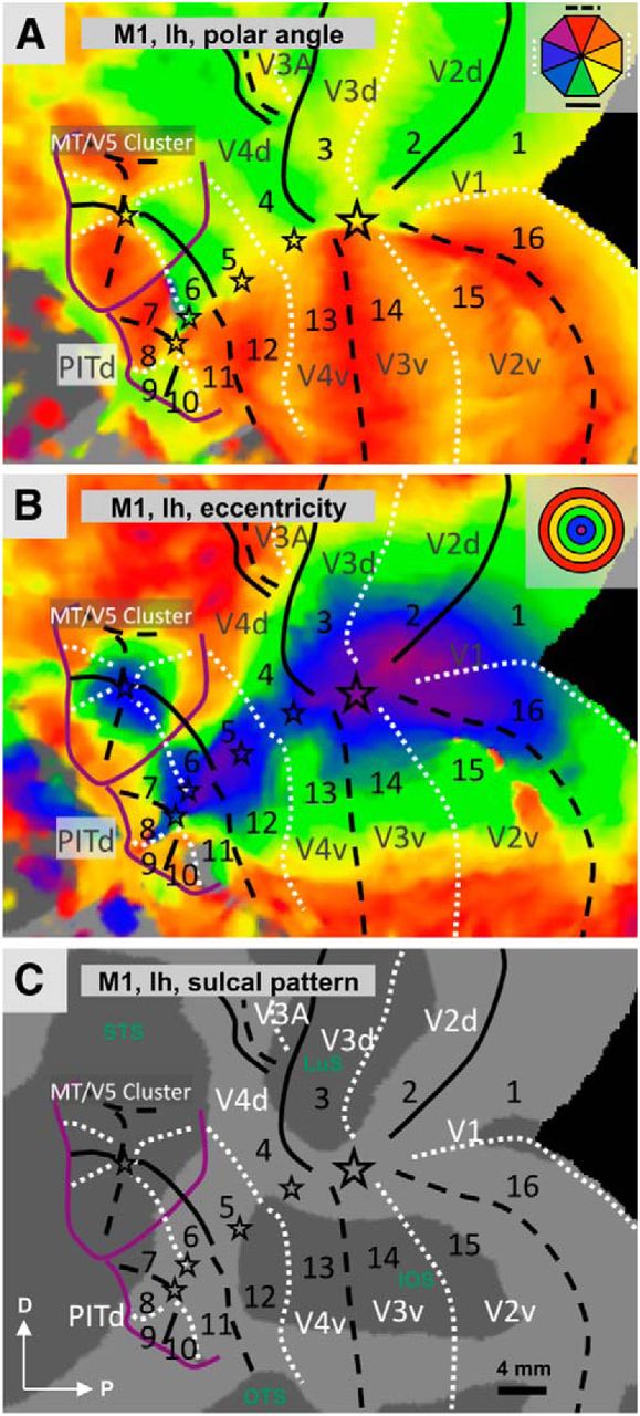
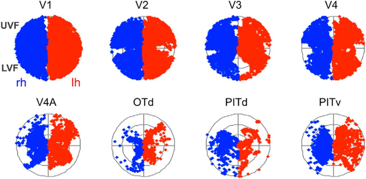
Monkey–human comparison. The visual areas are paired according to close similarity in topographic organization or pRF size. The color of the data points in A–C is matched with the colors of associated areas in Figure 19 and earlier. All error bars represent SEM across the two subject pools. R2 and t values are given for correlations between the two datasets. A, Absolute pRF sizes of monkey versus human. The dashed line represents positions of equal pRF sizes. The data are linearly correlated (solid gray line) with R2 = 0.92 and t = 10.8 (test for 0 correlation). B, fMRI response signal amplitudes for motion sensitivity, monkey versus human. The solid gray line represents a linear fit to the data with a coefficient of determination of R2 = 0.94 and t = 12.6 (test for 0 correlation). C, Response signal amplitudes for shape sensitivity, monkey versus human. The solid gray line represents a linear fit to the data with a coefficient of determination of R2 = 0.64 and t = 4.2 (test for 0 correlation). All data presented in A–C were collected using the same stimuli and analysis methods in both monkey and human experiments, while the hardware and type of activation were different: the monkey data were collected on a Siemens 3T scanner using CBV-fMRI with a strong negative contrast, while the human data were collected on a Philips 3T scanner using BOLD fMRI with a weaker positive contrast.
Although differences in the topographic organization of areas in these regions are observed, the differences may be explained by an evolutionary transformation of the human cortex compared with that of the monkey, while some functional similarities remain (Mantini et al., 2012, 2013). The weaker correlation (R2 = 0.64, t = 4.2) and shallower slope of the regression line found for shape compared with motion processing (R2 = 0.94, t = 12.6) might indicate different evolutionary paths of the dorsal and ventral stream areas in monkey and human. This is further supported by the observation that some of the shape-processing areas, which show the weaker overall correlation, underwent a topographic transformation in one species, while the motion-selective areas, which show the higher correlation, have a very similar topographic organization in both species (Fig. 19).
Future higher-resolution fMRI using different types of phase-encoded stimuli that are optimized for driving more anterior areas may be needed to resolve whether more anteriorly located regions show some degree of retinotopic organization. Ultimately, to increase our understanding of the representations of visual information in IT cortex, it will be also necessary to link its responses to highly specific visual stimuli, such as faces, bodies, places, and objects, with the retinotopic maps described here (Janssens et al., 2014).
Footnotes
- Received August 1, 2013.
- Revision received May 26, 2014.
- Accepted May 28, 2014.
This work was supported by Inter-University Attraction Pole 7/11, Programme Financing PFV/10/008, Geconcerteerde Onderzoeks Actie 10/19, Impuls financiering Zware Apparatuur and Hercules funding of the Katholieke Universiteit Leuven, Fonds Wetenschappelijk Onderzoek–Vlaanderen G062208.10, G083111.10, G0A56.13, G0439.12, K7148.11, and G0719.12. The Martinos Center for Biomedical Imaging is supported by National Center for Research Resources Grant P41RR14075. We thank C. Fransen, C. Van Eupen, and A. Coeman for animal training and care; S. Verstraeten, W. Depuydt, G. Meulemans, P. Kayenbergh, M. De Paep, and I. Puttemans for technical assistance; S. Raiguel for comments on the manuscript; and B. Rosen for his encouragement.
- Correspondence should be addressed to H. Kolster and W. Vanduffel, Laboratorium voor Neuro- en Psychofysiologie, KU Leuven Medical School, Campus Gasthuisberg, 3000 Leuven, Belgium. hauke.kolster{at}med.kuleuven.be; wim{at}nmr.mgh.harvard.edu
- Copyright © 2014 the authors 0270-6474/14/3410168-24$15.00/0