
Abstract
Early visual areas have neuronal receptive fields that form a sampling mosaic of visual space, resulting in a series of retinotopic maps in which the same region of space is represented in multiple visual areas. It is not clear to what extent the development and maintenance of this retinotopic organization in humans depend on retinal waves and/or visual experience. We examined the corticocortical receptive field organization of resting-state BOLD data in normally sighted, early blind, and anophthalmic (in which both eyes fail to develop) individuals and found that resting-state correlations between V1 and V2/V3 were retinotopically organized for all subject groups. These results show that the gross retinotopic pattern of resting-state connectivity across V1-V3 requires neither retinal waves nor visual experience to develop and persist into adulthood.
SIGNIFICANCE STATEMENT Evidence from resting-state BOLD data suggests that the connections between early visual areas develop and are maintained even in the absence of retinal waves and visual experience.
- blindness
- cortical maps
- fMRI
- resting state
- retinotopy
- visual deprivation
Introduction
Early visual deprivation disrupts ocular dominance column formation, receptive field size, and orientation, spatial frequency, direction, and disparity tuning (for review, see Hirsch and Leventhal, 1978; Movshon and Van Sluyters, 1981; Sherman and Spear, 1982; Rao and Jacobson, 2006; Ackman and Crair, 2014). In contrast, development of retinotopic organization is primarily driven by molecular signaling (Huberman et al., 2008; Cang and Feldheim, 2013). Retinotopic maps in the dorsal lateral geniculate nucleus and visual cortex of mice persist in the absence of retinal waves, although precision is reduced (Grubb et al., 2003; McLaughlin et al., 2003; Cang et al., 2005). In the macaque, adult-like connections between V1 and V2 are present before birth, shortly after LGN axons reach layer IV (Coogan and Van Essen, 1996), although further refinement occurs with the onset of visual experience (Barone et al., 1995; Batardière et al., 2002; Baldwin et al., 2012).
Little is known about how these connections are affected by long periods of deprivation. Sight recovery subjects retain basic visual abilities after long periods of deprivation (Fine et al., 2003; Sikl et al., 2013), and retinotopic organization has been demonstrated in an adult sight recovery subject blinded at 3 years of age (Levin et al., 2010), yet it is not clear whether the retinotopic pattern of connections between early visual areas is maintained in early blind and anophthalmic (in which input from the optic nerves never exists or only exists temporarily early in development before the embryonic eyes degenerate) individuals.
Furthermore, early blind and anophthalmic individuals show occipital functional responses during auditory (e.g., Collignon et al., 2009; Watkins et al., 2013), tactile (Sathian and Stilla, 2010), language (Bedny et al., 2011; Watkins et al., 2012), and verbal memory (Amedi et al., 2003) tasks (for review, see Lewis and Fine, 2011). It is not known whether these cross-modal responses replace or coexist with retinotopic patterns of connectivity.
Here, we examine the effect of anophthalmia and early blindness on the organization of resting-state BOLD correlations in visual cortex of humans. Slow fluctuations in the BOLD signal measured at rest show correlations across brain regions (Hagmann et al., 2008; Greicius et al., 2009; Honey et al., 2009; Bowman et al., 2012), which are thought to partially reflect neural activity (Biswal et al., 1995; Greicius et al., 2003). The occipital resting-state signal contains several components, including the following: (1) local spatial correlations (Butt et al., 2013, 2015); (2) large-scale iso-eccentric fluctuations within and across hemispheres (Heinzle et al., 2011; Jo et al., 2012; Butt et al., 2013, 2015; Haak et al., 2013; Gravel et al., 2014; Raemaekers et al., 2014; Arcaro et al., 2015); and (3) a component that maps to retinotopic organization. The clearest evidence for retinotopic organization, which cannot be explained by the other components, is the reversal in polar angle on the V2/V3 border (Heinzle et al., 2011; Gravel et al., 2014; Raemaekers et al., 2014).
Previous studies have found local spatial correlations (Butt et al., 2013, 2015), higher correlations between cortical areas representing the same region of visual space (Butt et al., 2015; Striem-Amit et al., 2015), and higher correlations between iso-eccentric locations (Butt et al., 2015; Striem-Amit et al., 2015), in both blind and sighted subjects (Table 1; see Discussion). However, these studies have not shown the V2/V3 polar angle reversal required to definitively demonstrate the retinotopic component of the resting-state signal persists following early blindness.
Selective summary of previous findings comparing the resting-state signals between blind and sighted individuals, including a description of which resting-state components would predict each findinga
We examined the organization of resting-state signals across visual areas by estimating ipsilateral “connective fields,” the Gaussian region in V1 that best predicts the resting-state BOLD responses of seed voxels in V2 and V3 (Haak et al., 2013; Gravel et al., 2014). Correlations between resting-state signals across these visual areas were retinotopically organized in all subject groups, suggesting the retinotopic pattern of intrahemispheric resting-state connectivity across V1-V3 develops and persists in the absence of retinal waves and visual experience.
Materials and Methods
Subjects
Table 2 provides subject details. At the University of Washington, resting-state data were collected on early blind (rsEBUW, N = 5, 2 females) and normally sighted controls (rsCONUW, N = 5, 3 females). For the normally sighted control subjects, we also collected data while subjects passively viewed retinotopic mapping stimuli. At the University of Oxford, resting-state data were collected on anophthalmic subjects (rsANOOx, N = 5, 2 females) and control subjects (rsCONOx, N = 7, 5 females). Because resting-state data were collected in two locations using slightly different protocols, data from anophthalmic and early blind subject groups were only compared with normally sighted controls scanned in the same location using the same protocol. The study was approved by the University of Oxford and the University of Washington Institutional Review Boards, and all subjects provided written informed consent.
Subject details for anophthalmic and early blind individualsa
MRI
Oxford
Scans were acquired using a 3 tesla Siemens Trio with a 12-channel head coil. One or more anatomical images were acquired for each subject using a standard T1-weighted, high-resolution anatomical scan of MP-RAGE (192 axial slices, 192 × 192 matrix, 1 × 1 × 1 mm3, TR = 2.04 s, TE = 4.7 ms, TI = 900 ms, FA = 8°). An independent components analysis of these resting-state data has been published previously (Watkins et al., 2012).
Resting-state.
Echo planar BOLD fMRI data were collected with whole-brain coverage (180 volumes; 34 axial slices, 64 × 64 matrix, 3 × 3 × 3.5 mm3, TR = 2.1 s, TE = 28 ms, FA = 89°, descending slice acquisition). Functional scans were obtained in a dark room with subjects instructed to keep their eyes closed.
University of Washington
Scans were acquired using a 3 tesla Philips Achieva with a 32-channel head coil. One or more anatomical images were acquired for each subject using a standard T1-weighted, high-resolution anatomical scan of MP-RAGE (176 slices, 256 × 256 matrix, 1 × 1 × 1 mm3, TR = 2.2 s, TE = 3.5 ms, TI = 896.45 ms, FA = 7°).
Resting-state.
Echo planar BOLD fMRI data were collected with whole-brain coverage (160 volumes, 43 axial slices, 80 × 80 matrix, 3 × 3 × 3 mm3, TR = 2.4 s, TE = 25 ms, FA = 79°, ascending slice acquisition). Functional scans were obtained in a dark room with subjects instructed to keep their eyes closed.
Stimulus-driven.
Echo planar BOLD fMRI data were collected with whole-brain coverage (160 volumes, 43 axial slices, 80 × 80 matrix, 3 × 3 × 3 mm3, TR = 2.4 s, TE = 25 ms, ascending slice acquisition). Functional scans were obtained while subjects maintained fixation on a central fixation cross. Visual stimuli were generated using MATLAB and the PsychToolbox (Brainard, 1997; Pelli, 1997) and back-projected by a calibrated LCD projector on a screen mounted in the bore of the magnet, which subjects viewed via a mirror fixed on the coil. fMRI responses were measured using a 2 degree drifting bar stimulus (as in Dumoulin and Wandell, 2008). For all sequences, the stimulated areas contained a counter-phase flickering checkerboard pattern (100% contrast, 0.5 cycles per degree) modulating at 8 Hz, and the display region was an annular aperture extending from 0.25 to 8 degrees eccentricity.
In the stimulus-driven dataset, it is presumed that BOLD modulations over time were driven by both spontaneous BOLD fluctuations and by the neural response to the time-varying stimulus. The stimulus-driven component should be retinotopically organized, as regions that represent similar regions in space show similar stimulus-driven responses over time. This dataset therefore provides a demonstration of our ability to estimate connective fields in the presence of a known retinotopic component. With this motivation in mind, connective fields for the stimulus-driven data were generated in the same way as the resting-state data.
Image preprocessing
Brain surfaces were reconstructed and inflated from the MP-RAGE images using the FreeSurfer (version 5.1) toolkit (http://surfer.nmr.mgh.harvard.edu/) as described previously (Dale et al., 1999; Fischl et al., 1999). Raw echo planar (volumetric) data were motion corrected with a six parameter, least-squares rigid body realignment routine, using the first functional image as a reference, and sinc interpolated in time to correct for the slice acquisition sequence using SPM (Wellcome Trust Centre for Neuroimaging, University College London, London). There were no significant differences in head motion across groups (mean rms head motion ± SD: rsANOOx = 0.2911 ± 0.3748; rsCONOx = 0.0948 ± 0.0850; rsEBUW = 0.1557 ± 0.0431; rsCONUW = 0.1362 ± 0.0390; stimCONUW = 0.1392 ± 0.0501). A one-way ANOVA revealed no differences in head motion across groups (F(1,4) = 0.81, p = 0.5334).
Following motion and slice timing correction, the echo planar data in subject space were coregistered (without interpolation) to a subject-specific anatomy in FreeSurfer using FSL-FLIRT with 6 df under a FreeSurfer wrapper (bbregister). Physiological noise was removed based on techniques of Jo et al. (2010). White matter, gray matter, ventricle, and nonbrain tissue ROIs were identified in each subject's anatomical image using Freesurfer and were subsequently projected to functional space. White matter, ventricle, and nonbrain tissue ROIs were eroded in 3D by 1 voxel to avoid any partial volume contamination by gray matter.
The influence of the average time courses for these three “noise ROIs” was removed from each gray matter voxel time course using linear regression. After noise removal, gray matter voxel time courses were high-pass filtered (0.01 Hz). A low-pass filter was not used because of concerns that low-pass filters have the potential to reduce sensitivity and induce artificial correlations in both task-related (Skudlarski et al., 1999; Della-Maggiore et al., 2002; Strother, 2006) and resting-state (Davey et al., 2013) fMRI data. Time courses were then projected to the corresponding (left or right) native cortical surface. The gray and black time courses in Figure 1C represent time courses before and after noise removal.

Schematic estimating the connective field for a seed voxel in V2 or V3. As described by Haak et al. (2013), assuming a linear relationship between blood-oxygenation levels and the fMRI signal, a predicted BOLD time course, p(t), can be calculated using a parametrized model of the connective field. A, The circular symmetric Gaussian model, g, is defined by its projection on a three-dimensional mesh representation of the boundary between the gray and white matter of the brain. Parameters consist of the Gaussian center location, v0 (in voxel coordinates) and the Gaussian spread, σ (in millimeters) across the folded cortical surface. B, The predicted BOLD time course, p(t), for any seed voxel is obtained by convolving the connective field, g(v0, σ), with the fMRI time course signals in V1. The connective field model parameters that best predict (C) the observed BOLD time course, y(t), are found by (D) maximizing the correlation coefficient between the prediction, p(t), and the observed time series, y(t). E, The parameter v0 is converted into visual space coordinates via the Benson template model of early visual areas (Benson et al., 2014). Parameters examined in this paper (r, σ, eccentricity, and polar angle) are bold underlined.
Cortico-cortico receptive field fitting
Seed voxels were selected from a large occipital ROI containing V2 and V3 (based on Freesurfer cortical parcellation), selected for each subject in native surface space. Connective fields for these seed voxels were estimated using custom software in MATLAB (The MathWorks), implementing a method closely related to that described by Haak et al. (2013). The connective field of each seed voxel within V1 (Fig. 1A) was modeled using a Gaussian function, g(v0, σ) with two parameters: v0 and σ as follows:
 where d(v, v0) is the shortest distance along the cortical surface mesh between voxels v (all V1 voxels in this case) and the connective field center v0, computed using the “graphshortestpath” function in MATLAB (using Dijkstra's algorithm). The parameter σ is the SD (mm) along the cortical surface.
We began by creating a set of fixed basis functions for each V1 voxel. These basis functions were described as Gaussians g(v0, σ) with center v0 corresponding to the surface vertex closest to that V1 voxel at the gray/white matter border. For each v0 value, we created 10 basis functions, using σ values linearly spaced between 3 and 25 mm. A series of predicted time courses were created for each V2 and V3 seed voxel by taking the linear sum of all V1 time courses convolved with all possible basis functions (Fig. 1B). The connective field for each V2/V3 voxel was initially defined as the parameters of the basis function g(v0, σ) that maximized the correlation between that V2/V3 voxel's time course and the resulting predicted time course. Initialization using this fixed set of σ values was critical for reducing the impact of local minima. It also had the advantage of shortening search time and excluding voxels with weak response modulation (for which the correlation with the initialization parameters was <0.1; under the assumption of linearity, this corresponds to a R2 of 0.01). This stage may also have also helped reduce the effect of bilateral symmetric resting-state components (Raemaekers et al., 2014).
The parameters of g(v0, σ) were then used to initialize a nonlinear search procedure (MATLAB simplex algorithm), which manipulated σ to maximize the correlation between the predicted and observed fMRI response time courses, holding v0 constant (Fig. 1C,D).
Conversion into visual space coordinates using the Benson template
Once the best fitting connective field was identified, connective field maps were projected to the corresponding hemisphere of a common FreeSurfer surface template (fsaverage) using the FreeSurfer spherical registration system (Fischl et al., 1999; Greve et al., 2011). The Benson template (2014) (details below) was used to convert v0 into retinotopic polar angle and eccentricity coordinates represented in terms of degrees of visual angle (Fig. 1E). This template was originally created for the left hemisphere, so we projected it onto the right hemisphere.
Seed voxels were excluded from further processing if they originated outside the Benson V1-V3 template (Fig. 2, dotted outlines). Unless otherwise stated, data were thresholded to only include connective fields for which the correlation between predicted and observed fMRI responses was >0.1 (set a priori). A similar pattern of results was found for all the results described below (including the phase reversal) for a more stringent threshold of 0.2.
The Benson template is not validated against older or blind subjects, and both age (Hogstrom et al., 2013) and early visual deprivation led to a small reduction in cortical folding (Dehay et al., 1989, 1996). However, the expected effect of a misaligned Benson template would be to reduce correlations, increase mean squared differences between predictions and the retinotopic template, and reduce the V2/V3 reversal effect, regardless of which direction the boundary is misaligned. Thus, misalignment of the template cannot contribute to our finding of retinotopically organized polar angle connective field estimates in blind individuals. Inspection of individual data found no evidence of systematic misalignment.
ROI selection
Areas V1-V3 were defined using an anatomical template of Benson et al. (2014), which uses surface topology to predict both polar angle and eccentricity. This template accurately predicts the location and retinotopic organization of V1 (Benson et al., 2012) or V1-V3 (Benson et al., 2014) in sighted subjects from cortical anatomy alone.
V2 and V3 ROIs were further partitioned into three equal subregions (“foveal,” “middle,” and “peripheral”) as a function of eccentricity based on the Benson template. The boundaries, which were chosen to produce equal numbers of voxels within each eccentricity band, were 5.5 and 18.9 degrees eccentricity for the left hemisphere, and 5 and 18.6 degrees for the right hemisphere. These two ROIs also correspond to the region of the template that has been empirically validated based on stimulus-driven retinotopic maps. The most peripheral boundary represented 18.6/18.9–83 degrees eccentricity, corresponding to the greatest eccentricity value represented in the Benson template.
ROIs were also partitioned into dorsal and ventral subregions. Ventral subregions were defined as those with a template polar angle value >90 (representing the upper visual field in normally sighted individuals); dorsal subregions were defined as those with a template polar angle value <90 (representing the lower visual field in normally sighted individuals).
Model of local resting-state correlations
We also compared our polar angle estimates with a model based purely on local spatial correlations in the resting-state signal, using parameters based on a previous study of resting-state fMRI (Butt et al., 2013). Random time courses were created across the entire cortical surface (using MATLAB's randn function). Local spatial correlations were then induced by smoothing these random time courses on the cortical surface using a 30 mm kernel. This produced simulated resting-state correlations on the cortical surface whose point spread of local spatial correlations (converted into z-scores) was best modeled by a Gaussian with σ of 20 mm, the value observed by Butt et al. (2013). Additional random noise was then added with an amplitude 200% of the original time course variance, so as to produce connective fields with median correlation coefficients of 0.292, similar to those observed in subject data (see below). Results using this model proved robust to a wide range of added noise (0%–2000% was tested). Cortico-cortico receptive field fitting (as described above) was carried out on these simulated time courses.
Statistics
Bootstrapping
As distributions of connective field values were non-normal, statistical comparisons adopted a nonparametric approach. Comparisons of frequency distributions of connective field parameter values across groups were performed using a bootstrapping procedure using custom software, based on the χ2 test of independence. This test compares the obtained frequency distributions for each group with those that would be obtained if the frequency distribution of connective field parameter values was independent of group assignment. We began with a classic χ2 test of independence, in which the obtained frequencies of the parameter value of interest were compared with the expected frequency distribution of connective field parameter values was independent of group assignment. Thus, a large χ2 value suggests that group membership influences the distribution of values obtained for that parameter (McHugh, 2013). The significance of the χ2 value was estimated using a bootstrapping procedure, which simply reestimated χ2 after randomly assigning subjects to groups (10,000 simulations). Significance was estimated as the probability of shuffled χ2 values exceeding the real χ2. Subjects (rather than voxels or hemispheres) were randomly assigned between groups.
When comparing distributions across the two hemispheres, we again randomly assigned subjects (rather than voxels) across groups, making this bootstrap procedure the equivalent of a random-effects analysis.
Comparing individual subject data to the Benson template/local correlations (LC) model
Eccentricity and polar angle connective field values in V2/V3 were compared with the V2/V3 values found in the Benson anatomical surface template, as well as the model based on local resting-state correlations, using R2 and mean squared difference (MSD) values.
MSD between the Benson template and individual data was calculated as follows for each individual hemisphere: MSDBenson =
The significance of R2 or MSD values was estimated using a bootstrapping procedure, where the real distribution of R2 or MSD values was compared with simulated distributions created using random assignment of subjects across the two groups (10,000 simulations). Once again, simulating bootstrapped distributions by randomly assigning subjects (rather than voxels) across groups made this bootstrap procedure the equivalent of a random-effects analysis.
Multiple comparisons
Correction for multiple comparisons was performed using Bonferroni–Holm correction (Holm, 1979), a sequentially rejective version of a simple Bonferroni correction for multiple comparisons, which controls the family-wise error rate at level α.
Results
Figure 2 shows the four parameters that represent our connective field model on the left hemisphere surface, averaged across all members of each subject group. The V2/V3 ROI used for analyses is shown with a dotted line. Figure 2A shows correlation coefficients. These provide a measure of the fit of the connective field model. Any deterioration in retinotopic organization might lead to a reduction in spatially local correlated neural firing, and thereby reduce correlation coefficients. Figure 2, B and C, shows eccentricity and polar angle parameters (in degrees of visual angle), respectively. These parameters provide a way of examining whether the match between connective field location and that predicted by retinotopic organization is disrupted by blindness. Finally, Figure 2D shows connective field size estimates (in millimeters). Expansion of connective field sizes might be expected if visual deprivation resulted in either an increase in receptive field size or a reduction in the precision of retinotopic organization, as increased scatter in receptive fields might serve to increase connective field size (Dumoulin and Wandell, 2008).

Connective field parameters of interest for V2/V3 on the surface of the left hemisphere, averaged across all members of each subject group. The V2/V3 ROI used in analyses is shown as a dotted outline. Columns from left to right represent the following: (A) the correlation between predicted and obtained time courses, (B) estimated eccentricity, (C) estimated polar angle, and (D) estimated σ (connective field size, mm on the cortical surface). Rows represent parameter estimates for resting-state anophthalmic subjects (Oxford), resting-state normally sighted Oxford controls, early blind subjects (UW), resting-state normally sighted UW controls, and normally sighted UW controls viewing retinotopic mapping stimulus sequences. The legend shows color coding for each subject/hemisphere. Top insets, Expected mappings for eccentricity and polar angle within V2 and V3 based on the Benson et al. (2014) template, with V1 outlined in black.
Correlation coefficients
Correlation coefficients were examined using an ROI that consisted of both V2 and V3. Our goal was to test for differences in correlation coefficients across groups, as might be expected if neural connectivity between V1 and V2/V3 was less precise or disrupted in blind individuals. We also wanted to make sure our threshold of 0.1 did not mask differences across subject groups.
Figure 3 shows probability distributions of correlation coefficients for all five subject groups. Each color in the stacked histogram represents the V2/V3 ROI in a separate individual hemisphere. The distribution of correlation coefficients for each hemisphere was normalized to sum to 1, so each hemisphere and subject contributes equally to the plot. A relatively small proportion of voxels were excluded because their connective field correlation coefficients fell below the threshold of 0.1 (percentage excluded: rsANOOx = 8.74%; rsCONOx = 8.12%; rsEBUW = 10.74; rsCONUW = 14.05; stimCONUW = 10.39%). Two-tailed Wilcoxon rank-sum tests did not find any significant differences across subject groups in the number of excluded voxels (rsANOOX vs rsCONOX: t(21) = −0.824, p = 0.419; rsEBUW vs rsCONUW: t(18) = 1.013, p = 0.325; rsCONUW vs stimCONUW: t(18) = −1.417, p = 0.174). Excluded voxels are shown as having a correlation of 0 in Figure 3.

Probability density distributions of connective field correlation coefficients (r). Each color in the stacked histogram represents a separate individual hemisphere. The legend shows color coding for each subject/hemisphere. The distribution of correlation coefficients for each hemisphere was normalized to sum to 1, so each hemisphere and subject contributes equally to the plot. Data are the following: (A) resting-state anophthalmic subjects (Oxford), (B) resting-state normally sighted controls (Oxford), (C) early blind subjects (UW), (D) resting-state normally sighted controls (UW), and (E) normally sighted controls (UW) viewing retinotopic mapping stimulus sequences.
Median correlation coefficients were ∼0.3, corresponding to R2 = 0.09 under an assumption of linearity (median values: rsANOOx = 0.304; rsCONOx = 0.324; rsEBUW = 0.403; rsCONUW = 0.282; stimCONUW = 0.337). Bootstrapped tests of χ2 independence (random effects) on the distribution of correlation coefficients that passed threshold found no effect of hemisphere on the distribution of correlation coefficients for any subject group.
We did see differences across groups for the distribution of correlation coefficients that passed threshold (Table 3). Bootstrapped χ2 tests of independence revealed that correlation coefficients were significantly higher for early blind subjects than for their sighted controls. The reason for this is not entirely clear (see Discussion). However, the finding that blind subjects had equal (or higher) correlation values than sighted subjects suggests that the use of a 0.1 threshold did not “bias” our results toward finding equivalent retinotopic organization in anophthalmic and early blind subjects, as might be the case if fewer retinotopically organized voxels passed threshold in these groups.
Group differences for connective field correlation coefficients in V2/V3 ROI
Correlation coefficients were also significantly higher for stimulus-driven compared with resting-state data (Fig. 3; Table 3), although this did not pass correction for multiple comparisons. This finding is likely due to the enhanced signal provided by the stimulus-driven neural fluctuations (see Discussion).
Eccentricity
Eccentricity estimates differ between foveal, middle, and peripheral ROIs
Connective field eccentricity estimates were also examined using an ROI consisting of both V2 and V3. Because χ2 estimates fail when a large number of cells have low expected probabilities, bin sizes were logarithmically distributed across the possible range of eccentricities when carrying out bootstrapped tests of χ2 independence for eccentricity. No difference between left and right hemispheres was found on the distribution of connective field eccentricity estimates for any subject group.
Figure 4 shows probability distributions of eccentricity estimates for all five subject groups for foveal, middle, and peripheral ROIs. The idealized histograms, estimated from the Benson template, are shown as insets for each column. Eccentricity values fall off with a approximately exponential distribution, as predicted by cortical magnification (Engel et al., 1997; Dougherty et al., 2003; Duncan and Boynton, 2003). If connective field estimates were “perfect,” the histogram for each ROI would fall completely within the shaded region. Indeed, connective field estimates collected for stimulus-driven data fell almost perfectly into the shaded region for foveal and middle ROIs. Connective field estimates for the peripheral ROI fall outside the shaded region. This is likely due to the fact that the retinotopic stimuli were presented within a visual field of 8° radius; thus, the region of visual field corresponding to this peripheral ROI did not receive visual stimulation.

Probability density distributions of connective field eccentricity parameters. Each color in the stacked probability distribution represents a separate hemisphere (see legend of Fig. 3). Data are the following: (A) resting-state anophthalmic subjects (Oxford), (B) resting-state normally sighted controls (Oxford), (C) early blind subjects (UW), (D) resting-state normally sighted controls (UW), and (E) normally sighted controls (UW) viewing retinotopic mapping stimulus sequences. Shaded regions represent the eccentricity boundaries for the V2/V3 foveal, middle, and peripheral ROIs, respectively. Top insets, Expected probability distributions for eccentricity within V2 and V3 based on the Benson et al. (2014) template.
Although most apparent for stimulus-driven data, connective field estimates were smaller for foveal compared with middle ROIs, as well as smaller for middle compared with peripheral ROIs, for all subject groups. The distribution of connective field eccentricity estimatesx differed significantly across both the foveal versus middle ROIs and between middle versus peripheral ROIs for all subject groups except rsCONUW (Table 4). Thus, eccentricity estimates followeddistribution of connective field eccentricity the expected general pattern of organization.
Connective field eccentricity estimates in V2/V3 ROI: foveal versus middle, and middle versus peripheral ROIs
Table 5 examines group differences in the distribution of eccentricity values. There was a significant difference between anophthalmic subjects and their sighted controls for the foveal ROI, but this did not pass correction for multiple comparisons. Visual inspection of the data of Figure 4 revealed that the peak in the foveal ROI probability distributions was shifted toward slightly larger eccentricity values in anophthalmic subjects compared with their sighted controls. If real, this difference in distributions might be interpreted as demonstrating a shallower slope for foveal cortical magnification.
Group differences for connective field eccentricity estimates in V2/V3 ROI
Comparison of eccentricity estimates with the retinotopic model
Finally, we compared connective field eccentricity parameters with Benson et al. (2014) template estimates of eccentricity, using both correlation coefficients (R2) and MSDs. The two measures differ slightly in their interpretation. MSD values represent the deviation between our obtained connective field values and the values predicted by the template. In contrast, high R2 values can be obtained even if the slope of cortical magnification differs from the slope predicted from the Benson template, as might be the case if the Benson template underestimated or overestimated cortical magnification in blind individuals. Correlations between eccentricity estimates from the connective field model and the Benson et al. (2014) template were significantly positive (p < 0.01, Bonferroni–Holm correction for five comparisons) for all individual subjects (rsANOOx: median R2 = 0.041, rsCONOx: median R2 = 0.081, rsEBUW: median R2 = 0.152; rsCONUW: median R2 = 0.087; stimCONUW: median R2 = 0.1510).
Correlation coefficients (after a Fisher z-score transform) and MSD values were compared across groups using unsigned Wilcoxon rank sum tests (Table 6). Neither test found differences between anophthalmic or early blind subjects and their sighted controls, but correlation coefficients were significantly higher for stimulus-driven compared with resting-state data, presumably due to visual stimuli eliciting a neural response, which enhances the retinotopic component of the fMRI signal.
Group differences for MSD and R2 values comparing connective field eccentricity estimates to the Benson et al. (2014) template
Thus, in all subject groups, our data show connective fields of V2/V3 mapping to iso-eccentric locations in V1, as would be expected if resting-state signals reflect retinotopic organization. However, it is important to note that, as discussed below, other groups have noticed a bilateral symmetric signal within the early visual areas, which, although nonretinotopic, would predict a very similar outcome (Heinzle et al., 2011; Jo et al., 2012; Butt et al., 2013, 2015; Haak et al., 2013; Gravel et al., 2014; Arcaro et al., 2015). Thus, the presence of mapping for eccentricity is necessary but not sufficient to demonstrate a retinotopic component within the resting-state signal.
Polar angle
As discussed more fully below, eccentricity and σ parameters closely resembling those that would be expected to arise from retinotopic organization can also manifest from a combination of local spatial correlations in the resting-state signal (Butt et al., 2013), and a global bilaterally symmetrical signal consisting of enhanced correlations between iso-eccentric regions (Raemaekers et al., 2014), which may arise from vasculature that symmetrically stems from the posterior cerebral artery (Tong et al., 2013; Tong and Frederick, 2014). Correspondence between polar angle parameter values and expected retinotopic organization is therefore critical for demonstrating that our connective fields are at least partially driven by correlations in neural firing that reflect retinotopic organization.
Polar angle estimates differ between dorsal and ventral ROIs
Figures 5 and 6 show probability distributions of polar angle estimates for all five subject groups for dorsal and ventral ROIs in V2 and V3, respectively. The Benson template for V1 is mirror symmetric, such that 0 represents the left horizontal median for right V1 and the right horizontal meridian for left V1. Consequently, polar angle estimates for left and right hemispheres can be combined without further transformation. Bootstrapped tests of χ2 independence did not find any difference between left and right hemispheres on the distribution of V2 and V3 connective field polar estimates for either ventral or dorsal ROIs for any subject group.

Probability density distributions of connective field polar angle parameters for V2v and V2d. Data are the following: (A) resting-state anophthalmic subjects (Oxford), (B) resting-state normally sighted controls (Oxford), (C) early blind subjects (UW), (D) resting-state normally sighted controls (UW), and (E) normally sighted controls (UW) viewing retinotopic mapping stimulus sequences. Shaded regions represent expected polar angle boundaries for dorsal and ventral ROIs. Top insets, Expected probability distributions for polar angle within V2 and V3 based on the Benson et al. (2014) template.
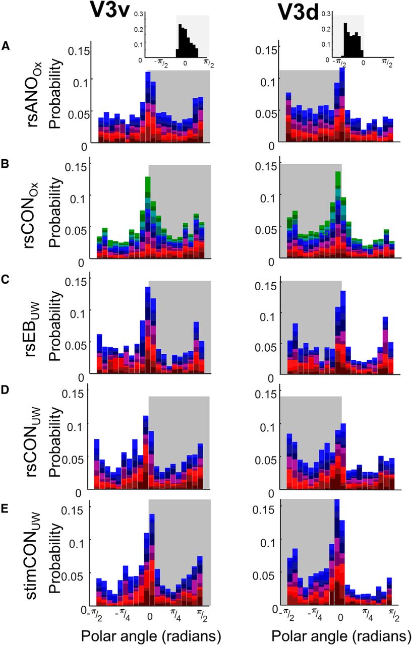
Probability density distributions of connective field polar angle parameters for V3v and V3d. Data are the following: (A) resting-state anophthalmic subjects (Oxford), (B) resting-state normally sighted controls (Oxford), (C) early blind subjects (UW), (D) resting-state normally sighted controls (UW), and (E) normally sighted controls (UW) viewing retinotopic mapping stimulus sequences. Shaded regions represent polar angle boundaries for dorsal and ventral ROIs. Top insets, Expected probability distributions for polar angle within V2 and V3 based on the Benson et al. (2014) template.
As seen from the inset (based on the Benson template), ventral ROI connective field estimates of polar angle should be distributed between 0 and π/2, whereas dorsal ROI estimates of polar angle should be distributed between 0 and −π/2. Bootstrapped tests of χ2 independence (Table 7) found that in V2 the distribution of connective field polar angle estimates differed significantly across ventral and dorsal ROIs for all subject groups. In V3 differences across ventral and dorsal ROIs only reached significance in Oxford resting-state control subjects, and this did not survive correction for multiple comparisons.
Connective field polar angle estimates: ventral versus dorsal for V2 and V3
The only group differences found for the distribution of connective field polar angle estimates were within V2d (rsANOOX vs rsCONOX: χ(19)2 = 915.879, p = 0.042; rsCONUW vs stimCONUW: χ(19)2 = 1203.594, p = 0.004). Only the difference between stimulus-driven and resting-state data passed Bonferroni–Holm correction for three comparisons.
Polar angle values within V2 and V3
We then examined the distribution of connective field estimates of polar angle within V2 and V3. Voxels within V2 and V3 were binned based on their expected polar angle representation using the Benson template. The mean connective field polar angle value for each bin is shown with solid symbols in Figure 7 (left panels). Because neither the Benson template nor the LC model incorporates hemispheric differences, we treated each hemisphere as a separate “subject,” so SEs reflect individual hemispheres. Connective field polar angle values predicted by the Benson template are shown with a solid line. Connective field polar angle values produced by a model of LC are shown with empty circles. As might be expected, connective fields in the LC model often have the same polar angle as the closest V1 location, resulting in polar angle estimates clustered at ∼±π/2. This “step” pattern was seen for a variety of noise levels (60%–1000% of time course variance).

Left panels, Connective field estimates of polar angle for all 5 subject groups. Data are the following: (A) resting-state anophthalmic subjects (Oxford), (B) resting-state normally sighted controls (Oxford), (C) early blind subjects (UW), (D) resting-state normally sighted controls (UW), and (E) normally sighted controls (UW) viewing retinotopic mapping stimulus sequences. Voxels were binned based on their expected polar angle representation, using the Benson template. Solid symbols represent means across individual hemispheres. SEs across individual hemispheres are shown. Solid lines indicate predicted mean connective field estimates of polar angle based on the Benson template. Open circles represent predicted estimates based on the LC model. Right panels, Histograms of MSDBenson − MSELC for each individual subject hemisphere. Negative values (left of the dotted line) imply that the Benson template provides a better fit than the LC model.
Connective field estimates within both V2 and V3 were closer to the predictions of the Benson template than the LC model. The x-axes of the histograms of Figure 7 (right panels) represent MSDBenson − MSDLC. Thus, negative values represent a better fit by the Benson template compared with the LC model. Wilcoxon signed rank tests found that the median of the distribution of MSD across individual hemispheres was significantly smaller for the Benson template for all subject groups (p < 0.001).
Last, we explicitly looked for the expected reversal across the V3/V3 border. In V2, the median of the distribution of correlation values (transformed into z-scores) between individual subject hemisphere polar angle estimates and the Benson template was significantly (Wilcoxon signed rank test) greater than zero for all groups (Table 8).
Correlations between connective field polar angle estimates and the Benson et al. (2014) template for V2 and V3
Correlations with the template were lower in V3 than V2, especially V3d. This is not surprising: the Benson template is less accurate for V3 than V2 (Benson et al., 2014). Moreover, retinotopic mapping tends to be less robust dorsally than ventrally, and is less robust in V3 than within V2. Within V3, we found significantly positive correlations between subject data and the Benson template for anophthalmic subjects, Oxford sighted controls, and UW sighted subjects viewing retinotopic stimuli. The failure to find significantly positive correlations within V3 for early blind subjects and their sighted controls is likely due to lower signal-to-noise within the University of Washington scanner rather than a genuine difference between early blind and anophthalmic subjects, given that it was found in both subject groups.
Given the complexity of the resting-state signal in early visual areas, which likely includes bilateral symmetrical fluctuations that can produce the artifactual appearance of eccentricity mapping, a critical finding of our data is that we can successfully find the polar angle reversal at the V2/V3 border using resting-state as well as stimulus-driven data: at least in anophthalmic subjects, their sighted controls, and UW stimulus-driven control subject data. This reversal is a strong test of retinotopic organization, as it is difficult to think of any realistic model of spatial or vascular correlations that would predict such a finding.
Connective field size
No difference between left and right hemispheres was found on the distribution of connective field size estimates for any subject group for either the V2 or the V3 ROI. To improve our ability to sample the joint probability distribution describing connective field size and eccentricity, each hemisphere was treated as a separate “subject” rather than carrying out separate analyses for left and right hemispheres.
Figure 8 shows the joint probability distribution for connective field size and eccentricity, for each subject group for V2 and V3. Because χ2 estimates fail when a large number of cells have low expected probabilities, bin sizes for eccentricity were unevenly distributed across the range of possible sizes (bin widths of 0.25 between 0 and 3, widths of 0.5 between 3 and 6, and widths of 3 between 6 and 15 mm). Results were robust to the particular choice of bin sizes.

Two-dimensional joint probability distributions (x-axis, connective field size; y-axis, eccentricity) of connective field size as a function of eccentricity for V2 and V3. Data are the following: (A) resting-state anophthalmic subjects (Oxford), (B) resting-state normally sighted controls (Oxford), (C) early blind subjects (UW), (D) resting-state normally sighted controls (UW), and (E) normally sighted controls (UW) viewing retinotopic mapping stimulus sequences. The third column represents the differences between the joint histograms of V2 and V3. For reasons of visualization, the range of connective field sizes is limited to 0°-6°.
Differences in connective field sizes between V2 and V3
The resting-state connective field sizes shown in Figure 8 are very similar to those previously observed by Gravel et al. (2014) in normally sighted subjects, who found V2 and V3 had similar connective field sizes of ∼2 mm. Differences between V2 and V3 were small and consisted of connective fields in V2 being smaller than those in V3 for all but the largest eccentricities (Fig. 8, third column, difference maps). This difference between V2 and V3 was only significant for rsCONOx and stimCONUW, and only the latter result passed correction for multiple comparisons (Table 9).
Connective field size estimates: median sizes of connective fields in V2 versus V3, and the results of χ2 test examining whether the distribution of connective field sizes differed significantly between V2 and V3
Connective field size as a function of eccentricity
The bright vertical strips found within Figure 8 (left panels) indicate that connective field sizes remained relatively constant as a function of eccentricity, resembling previous findings that increases in ipsilateral connective field size as a function of eccentricity are small (Haak et al., 2013; Gravel et al., 2014). However, although small, the effects of eccentricity are statistically significant. Standard χ2 tests of independence found highly significant (p < 0.01) interactions between connective field size and eccentricity within both V2 and V3 for every subject group, using both the group averaged joint probability distributions of Figure 8, and when analyzing each individual hemisphere separately.
Comparison of subject groups found no differences between blind subjects and their sighted controls in the distribution of connective field sizes as a function of eccentricity within either the V2 or the V3 ROI (Table 10). There was a significant difference between resting-state versus visual stimulation in sighted controls within both V2 and V3, which was due to smaller connective fields for resting-state than for stimulus-driven data (see Discussion).
Group differences in connective field size in V2 and V3
Discussion
Resting-state correlations in occipital cortex
The occipital resting-state signal contains multiple components. One component consists of local spatial correlations, such that BOLD response similarity falls off smoothly as a function of cortical distance, which may reflect spatial spread inherent to the BOLD signal (Engel et al., 1997; Parkes et al., 2005). There are also large-scale iso-eccentric fluctuations within and across hemispheres. These fluctuations are bilaterally symmetric, correlations across hemispheres are stronger for homologous cortical locations representing symmetric regions of visual space (Heinzle et al., 2011; Jo et al., 2012; Butt et al., 2013, 2015; Haak et al., 2013; Gravel et al., 2014; Raemaekers et al., 2014; Arcaro et al., 2015), and may reflect vasculature stemming from the posterior cerebral artery (Tong et al., 2013; Tong and Frederick, 2014). The resting-state component that maps to retinotopic organization, including the polar angle V2/V3 reversal (Heinzle et al., 2011; Gravel et al., 2014; Raemaekers et al., 2014), seems to explain a relatively small proportion of resting-state variance. Our connective fields produced mean correlations between predicted and obtained time courses in V3 that ranged between r = 0.307 and r = 0.416. Similarly, using resting-state data, Heinzle et al. (2011) reported correlations between predicted and obtained time courses of r = 0.21 within V3. In contrast, stimulus-driven data produced correlations of r = 0.812 in V3 (Haak et al., 2013).
The connective field method may help emphasize retinotopic components of the resting-state signal, provided care is taken to avoid local minima. Suppose a seed voxel in V2 is strongly correlated with every iso-eccentric location in V1 (due to the bilateral symmetric component) but is most strongly correlated with the location of the same polar angle coordinate. Despite the retinotopic component being relatively weak, the resulting connective field will settle in the location of the retinotopic signal, as this method finds the point of maximum correlation between a seed voxel in V2 and a Gaussian region in V1.
Our finding of retinotopically organized polar angle estimates across the V2/V3 border suggests that our connective field estimates are sensitive to the retinotopic component within the resting-state signal, although it remains unclear to what extent our estimates were also influenced by nonretinotopic components. Possible future directions for better isolating the retinotopic component of the resting-state signal include using longer resting-state sequences or smaller voxel sizes at 7T (Raemaekers et al., 2014), using methods (e.g., independent component analysis) for factoring out non-neural (Tong and Frederick, 2014) or nonretinotopically organized signals, and improved connective field model fitting methods (e.g., global search algorithms) to avoid local minima induced by nonretinotopic components.
Differences between early blind and sighted individuals
One well-established finding, not reexamined in this study, is the observation that early blindness (Bedny et al., 2011; Qin et al., 2013; Burton et al., 2014) and anophthalmia (Watkins et al., 2012) result in a decrease in interhemispheric functional correlations, with the effect of blindness tending to increase across the visual hierarchy. However, there are a number of reasons to believe these interhemispheric correlations reflect iso-eccentric fluctuations rather than retinotopic patterns of connectivity (Bock and Fine, 2014).
An interesting finding of Butt et al. (2015), replicated here, is that although there is little difference in the spatial spread of intrahemispheric spatial correlations between blind and sighted subjects, correlation values in the resting-state signal are higher for early blind subjects compared with sighted controls. One possible explanation is that resting-state firing rates are increased and/or metabolic processes are enhanced within the occipital cortex as a result of early blindness. Dark-reared animals show high spontaneous firing rates within occipital cortex (for review, see Movshon and Van Sluyters, 1981) and early blind individuals show enhanced metabolic activity in occipital cortex, which might enhance the BOLD resting-state signal (Wanet-Defalque et al., 1988; Veraart et al., 1990; Uhl et al., 1993; De Volder et al., 1997; Weaver et al., 2013). Although it is not known whether anophthalmia leads to similar enhancements of metabolic activity and/or resting-state firing, we saw no difference in correlation coefficients between anophthalmic subjects and their sighted controls.
Stimulus-driven versus resting-state connective fields
As seen previously (Heinzle et al., 2011; Gravel et al., 2014; Raemaekers et al., 2014), we found higher correlation coefficients and clearer organization for eccentricity and polar angle in stimulus-driven compared with resting-state data, likely due to larger retinotopically organized neural fluctuations produced by the presence of a visual stimulus.
Similar to Raemaekers et al. (2014), estimated connective fields were smaller for resting-state than for stimulus-driven data within V2 and V3. These size differences are unlikely to be due to lower neural signal in resting-state data because connective field size estimates are an unbiased statistic (Dumoulin and Wandell, 2008; Binda et al., 2013), the reliability of connective field size estimates will be affected by signal-to-noise, but the mean size estimate is robust to signal-to-noise. There are several possible explanations for finding smaller connective fields as follows: (1) the local spatial correlations in the resting-state fMRI signal have a narrower spatial spread compared with the stimulus-driven retinotopic signal (Heinzle et al., 2011; Butt et al., 2013). In the absence of a visual stimulus, these LC would be more influential on the fMRI signal, producing a smaller connective field size. (2) Connective field sizes for stimulus-driven data may be inflated by nonlinear spatiotemporal BOLD interactions. (3) Neural responses related to the predictability of the drifting bar stimulus increase connective field size (Binda et al., 2013). (4) The drifting bar stimulus is weighted toward low spatial frequencies, which might result in BOLD response fluctuations being more influenced by neurons with larger receptive fields (Binda et al., 2013).
If differences in connective field parameters between stimulus-driven and resting-state conditions prove local to cortical regions representing the stimulated visual field, these differences may provide a method for mapping cortical regions with residual visual field function in cognitively impaired individuals with cortical visual impairment. Although collecting MR data in these individuals will generally require sedation, many undergo MR scans for medical reasons. Traditional perimetry tests are often impossible in these individuals, so estimating regions of spared vision is done on the basis of spontaneous behavioral responses, which is difficult and imprecise. Because caregivers are instructed to present items of interest in the spared visual field, an improved ability to estimate spared regions would have clinical value.
Does residual topographic organization interact with cross-modal responses?
We find here that neither retinal waves nor visual experience is necessary for the development and maintenance of retinotopic organization within resting-state signals. This is consistent with an animal literature suggesting that the refinement of intracortical visual circuitry is robust to loss of visual input (Coogan and Van Essen, 1996; Grubb et al., 2003; Cang et al., 2005; Ko et al., 2014). Molecular signaling plays a crucial role in the development of retinotopic maps (Huberman et al., 2008; Cang and Feldheim, 2013), although spontaneous propagating waves of activity within the retina (Demas et al., 2003; McLaughlin et al., 2003) (and possibly the lateral geniculate nucleus, Weliky and Katz, 1999), and postnatal visual experience (Barone et al., 1995; Batardière et al., 2002; Baldwin et al., 2012) play a role in the refinement of these maps.
Nonetheless, it is surprising that retinotopic organization of the resting-state signal persists in blind humans, even after many years of deprivation, especially given the presence of cross-modal responses to auditory and tactile stimuli within these same regions of cortex. As described above, there is a large literature showing occipital cross-modal responses as a result of blindness, and robust cross-modal responses have been previously observed in the particular subjects of this study (Watkins et al., 2013; Jiang et al., 2014). Our results suggest that these cross-modal responses coexist with neural firing patterns that reflect persisting retinotopic organization (also see Striem-Amit et al., 2015).
Cross-modal responses can coexist with visual responses in both occipital cortex and hMT+. Sight recovery subject MM was blinded at 3.5 years of age and regained limited vision at 43. Even after sight recovery, MM shows cross-modal responses within occipital cortex and hMT+ (Saenz et al., 2008; Jiang et al., 2014) that coexist with persisting retinotopic organization in occipital cortex (Levin et al., 2010) and visual motion responses in hMT+ (Saenz et al., 2008; Jiang et al., 2014).
How might the topographically organized firing patterns observed in our data interact with cross-modal responses? One possibility is that retinotopic responses are orthogonal to cross-modal responses and are merely a persistent artifact of early development. A more interesting possibility is that this topography may influence auditory or tactile responses. Cross-modal auditory motion responses in hMT+ responses share topographic similarities with restored visual motion responses: In MM it is possible to use BOLD responses in hMT+ to classify the direction of auditory motion stimuli based on a visual motion training set, and vice versa (Jiang et al., 2014). An obvious future direction is to examine whether cross-modal responses (such as auditory frequency tuning or spatial localization) might be topographically aligned with the retinotopic organization within early visual areas.
Footnotes
- Received November 15, 2014.
- Revision received June 24, 2015.
- Accepted July 10, 2015.
This work was supported by National Institutes of Health Grant R01 EY014645 to I.F., H.B. is a Royal Society University Research Fellow.
The authors declare no competing financial interests.
- Correspondence should be addressed to either of the following: Dr. Andrew S. Bock, Department of Neurology, University of Pennsylvania, Philadelphia, PA 19104, bock.andrew{at}gmail.com; or Dr. Ione Fine, Department of Psychology, University of Washington, Seattle, WA 98177, ionefine{at}uw.edu
- Copyright © 2015 the authors 0270-6474/15/3512366-17$15.00/0