
Abstract
Reliable timing of cortical spikes in response to visual events is crucial in representing visual inputs to the brain. Spikes in the primary visual cortex (V1) need to occur at the same time within a repeated visual stimulus. Two classical mechanisms are employed by the cortex to enhance reliable timing. First, cortical neurons respond reliably to a restricted set of stimuli through their preference for certain patterns of membrane potential due to their intrinsic properties. Second, intracortical networking of excitatory and inhibitory neurons induces lateral inhibition that, through the timing and strength of IPSCs and EPSCs, produces sparse and reliably timed cortical neuron spike trains to be transmitted downstream. Here, we describe a third mechanism that, through preferential thalamocortical synaptic connectivity, enhances the trial-to-trial timing precision of cortical spikes in the presence of spike train variability within each trial that is introduced between LGN neurons in the retino-thalamic pathway. Applying experimentally recorded LGN spike trains from the anesthetized cat to a detailed model of a spiny stellate V1 neuron, we found that output spike timing precision improved with increasing numbers of convergent LGN inputs. The improvement was consistent with the predicted proportionality of  for n LGN source neurons. We also found connectivity configurations that maximize reliability and that generate V1 cell output spike trains quantitatively similar to the experimental recordings. Our findings suggest a general principle, namely intra-trial variability among converging inputs, that increases stimulus response precision and is widely applicable to synaptically connected spiking neurons.
SIGNIFICANCE STATEMENT The early visual pathway of the cat is favorable for studying the effects of trial-to-trial variability of synaptic inputs and intra-trial variability of thalamocortical connectivity on information transmission into the visual cortex. We have used a detailed model to show that there are preferred combinations of the number of thalamic afferents and the number of synapses per afferent that maximize the output reliability and spike-timing precision of cortical neurons. This provides additional insights into how synchrony in thalamic spike trains can reduce trial-to-trial variability to produce highly reliable reporting of sensory events to the cortex. The same principles may apply to other converging pathways where temporally jittered spike trains can reliably drive the downstream neuron and improve temporal precision.
- feedforward
- lateral geniculate nucleus
- spike time variability
- spiny stellate cell
- thalamocortical connectivity
- visual cortex
Introduction
Timing precision in cortical spike trains is critical in representing visual images in the brain (von der Malsburg, 1995; Shadlen and Movshon, 1999; Butts et al., 2010). A pioneering in vitro experiment (Mainen and Sejnowski, 1995) showed that the timing of spikes can be highly precise and reliable when a fluctuating current waveform is repeatedly injected into cortical neurons. This established the conditions under which the intrinsic cell properties for spike initiation were capable of high temporal precision. Later in vivo recordings (Haider et al., 2010) demonstrated that network properties, including lateral inhibition and recurrent excitation from non-classical receptive fields (RFs), also enhance precise and reliable spike timing in visual cortex.
Experiments in cats and monkeys using fluctuating visual stimulation have revealed reliable spiking patterns in neurons throughout the visual pathway (Tanaka, 1983; Reid and Alonso, 1995; Gur et al., 1997; Zador and Dobrunz, 1997; Buracas et al., 1998; Kara et al., 2000; Reinagel and Reid, 2000, 2002; Butts et al., 2007, 2010; Kumbhani et al., 2007; Desbordes et al., 2008, 2010; Haider et al., 2010). The timing of these firing patterns, averaged over many trials, in the recorded cells, had a precision that varies from <1 ms SD (Reid and Alonso, 1995; Reinagel and Reid, 2002) to >10 ms (Buracas et al., 1998) in the lateral geniculate nucleus (LGN) and cortex.
Here, we explore intra-trial variability, arising from thalamocortical connectivity at the synaptic level, as a third mechanism for maintaining precision and reliability of behavioral event timing in the primary visual cortex (V1). Thalamic spike trains from in vivo cat experiments (Kara et al., 2000) were used to drive a multi-compartment/multi-synapse model of a layer-4 spiny stellate neuron in area V1 of the cortex. These short spike trains, from a drifting grating stimulus, had a 7-ms variability (one σ) in first spike timing from trial to trial. Alone, this inter-trial variability in the LGN induced a much larger timing variability in the layer-4 cortical neuron model. We found that the configuration of thalamocortical connectivity in the model, which closely matched that in the cat, significantly enhanced the reliability and precision of V1 cortical cell event timing. These timing improvements, which depended upon the number of activated afferent LGN cells and the total number of synapses per LGN axon, resemble the effects of intrinsic neuron properties (Mainen and Sejnowski, 1995) and intra-cortical connectivity (Haider et al., 2010).
A further source of intra-trial timing variation is the RF spread of each LGN cell. We found connectivity and RF parameters that produced model V1 output statistically similar to the V1 recordings taken from the same animals and at the same time as the LGN recordings (Kara et al., 2000). The configuration was found by choosing parameters that produced spike trains with characteristics that matched the recorded spike data across trials on multiple dimensions. The values of these parameters from the model (e.g., number of LGN afferents per V1 cell and average number of synapses per afferent) generally agree with the literature on layer-4 spiny stellate cells in cats (da Costa and Martin, 2009, 2011).
The convergence of input from multiple LGN cells onto a V1 cell is another mechanism for conveying visual event timing. This relationship between the connectivity of the synchronous presynaptic cells to the reliability and precision of the postsynaptic cell spike trains depended only on the presence of trial-to-trial variability in the input spike trains. It should apply generally to other such synaptically connected neurons and may be crucial both for efficient transfer of sensory information to cortex and for synchrony-based neural codes for communication and processing upstream in higher brain regions.
Materials and Methods
Experimental recordings.
The LGN inputs to our model were derived from a series of in vivo experiments in anesthetized adult cats, which simultaneously recorded from retinal ganglion cells, LGN relay cells, and simple V1 cells (Kara et al., 2000). The cells were not monosynaptically connected. The stimuli in these experiments were 4-Hz drifting sinusoidal gratings with 50% contrast, which were aligned with the preferred orientation of the V1 simple cell's RF. Figure 1A shows the visual stimulus with the output rastergram recorded from the LGN.

LGN input and structure of biophysical V1 model. A, LGN spike times recorded by Kara et al. (2000), from anesthetized cat in response to 4-Hz drifting sinusoidal grating at 50% contrast. Spike trains sorted into 250-ms segments and delivered as LGN input to the V1 model. B, Modeled system boxed within dotted lines, including driving LGN excitatory input, feedforward inhibition from a simple basket cell, and background excitatory and inhibitory input representing cortical activity, simulated in NEURON (Hines and Carnevale, 1997). All inputs fed into a layer-4 spiny stellate cell model (Mainen and Sejnowski, 1996), whose outputs were studied in this article.
The dataset used in this study came from four experiments in which recordings were made from a total of three LGN cells. Two of these were simultaneously recorded in the same animal (along with one retinal cell and one V1 cell) while the other came from another experiment (retinal cell + LGN cell + V1 cell). Only two cells (retinal + V1) were recorded in each of the two remaining experiments.
Although not purely Gaussian, the variability in the first spike time from over 800 trials of a single LGN neuron (Kara et al., 2000) has enough symmetry that SD is a useable comparative measure, as seen in Figure 2. Other investigators have observed jitter in the event-related spike trains from sensory pathways (Gur et al., 1997; Xu-Friedman and Regehr, 2005a,b; Kumbhani et al., 2007; Desbordes et al., 2008; Jeanne and Wilson, 2015). Various studies and analyses have found the trial-to-trial variation in the first spike latency to vary widely depending on the stimulus used, running the gamut from Gaussian distributed to alpha distributed (Xu-Friedman and Regehr, 2005b). The Kara LGN latency data of Figure 2 (SD 7.3 ms), is in general agreement with that of similar stimulus protocols in the anesthetized cat LGN (Kumbhani et al., 2007; Desbordes et al., 2008; Herikstad et al., 2011).

Spike jitter in LGN Spike trains is nearly Gaussian. Event-aligned rasters of spike times from the LGN cell (LGNA) used to drive model inputs (see Materials and Methods), sorted by first spike time (A–C) and by third spike time (D–F). Values of μ are α represent the mean and SD of the best-fit normal distributions to the observed spike time distributions (B, E). Quantile-quantile (Q-Q) plots compare quantiles of observed spike time distributions to quantiles of best-fit normal distributions (C, F). First spike times are non-normal (B, p < 0.05) but nearly so (C). Third spike times are normal (E, F, p > 0.05). Distributions of other spike times are non-normal (p < 0.05; data not shown). Non-normality p values determined by Shapiro–Wilk W test (Royston, 1992).
As suggested by Figure 2A, the time difference between the first spike and second spike is much less than the first spike variation. The distribution of first inter-spike interval (ISI), however, is decidedly non-Gaussian because it cannot be less than zero. A useful non-parametric measure in this case is the interquartile range used by Kumbhani and others (Kumbhani et al., 2007; Herikstad et al., 2011), which gives the middle 50% of values. The interval between first and second spike in these data has a mean of 2.7 ms and an interquartile range 0.6 ms, whereas the first spike time for this LGN cell varies with an interquartile range of 9.7 ms. For comparison, Kumbhani reported 8.1-ms interquartile range for first spike time in LGN X cells (Kumbhani et al., 2007), using fixed Gabor patches with varying contrast as the visual stimulus.
With one exception, all modeling and simulations shown in the figures are from the same LGN neuron recording in Figure 2 (designated LGNA). In most cases, this permits a more direct comparison of results. Other simulations have indicated our results do not change significantly when using the other LGN spike trains as inputs, either singly or as a large group. We ran V1 simulations to compare parametric thalamocortical connectivity models for all combinations of the experimentally recorded three LGN neurons and four V1 neurons.
Each of the four cat experiments recorded a single simple cell from layer-4 V1 (Kara et al., 2000). To tune and cross-validate our V1 spiny stellate cell model, we calculated the same metrics on the experimentally recorded V1 spike trains as on our model outputs (see below). The recorded data had a Schreiber reliability of 0.42, a Fano factor (FF) of 0.33, a mean spike rate of two to four spikes per trial, and a first spike precision of 18 ms−1.
Biophysical V1 model overview.
All simulations were performed in the NEURON simulation environment (Hines and Carnevale, 1997). We used a digitally reconstructed spiny stellate cell of the cat V1, layer 4 (Mainen and Sejnowski, 1996), consisting of 744 compartments, subdivided into 6 dendritic branches. We also simulated a feedforward inhibitory neuron that received input from LGN relay cells and contacted the spiny stellate cell (Fig. 1B). The inhibitory basket cell was adapted from Bush et al. (1999) and was downloaded from ModelDB (Hines et al., 2004). The V1 model included five currents: a fast Na+ current, a delayed rectifier K+ current, a slow non-inactivating K+ current, a slow after-hyperpolarization Ca2+-activated K+ current, and a high-voltage activated Ca2+ current. Complete details of the model, including a parameter list for all currents, are given in a previous paper and its associated supplemental information (Wang et al., 2010a). For a comparison to the parameters employed in another biophysically realistic V1 spiny stellate cell model, see Banitt et al. (2007).
All models ran for a total of 350 ms of simulation time per trial, with a time step of 0.1 ms and an initial 100 ms to allow the neuron to settle to baseline before delivering thalamocortical stimulation. To simulate background cortical activity, the V1 spiny stellate cell received afferents from 4500 intra-cortical (e.g., from L4 and L6) excitatory glutamatergic synapses and 1100 intra-cortical inhibitory GABAergic synapses, based on experimental estimates (Ahmed et al., 1994; Anderson et al., 1994; Stratford et al., 1996). Unless otherwise noted, all excitatory synapses were uniformly and randomly distributed throughout the dendritic tree and soma, while the inhibitory inputs resided perisomatically on dendrites within 200 μm of the soma. Background inputs fed each synapse of the spiny stellate cell with near-Poisson spike trains (1 Hz excitatory, 5 Hz inhibitory; Destexhe and Paré, 1999), which included a 2-ms refractory period between spikes and which updated randomly for each trial. In addition, the model received up to 300 excitatory synaptic contacts from the simulated LGN, treated as the main input to the model, and 200 feedforward inhibitory synapses from the basket cell. The total number of thalamocortical connections is based on anatomical measurements (Ahmed et al., 1994; Gil et al., 1999).
In contrast to inhibitory synapses, where release occurred with the arrival of each spike in the presynaptic train, the excitatory synapses from both the LGN and intra-cortical connections exhibited short-term facilitation and depression (Dobrunz and Stevens, 1997) with stochastic release (Allen and Stevens, 1994). This dynamic stochastic synapse model was based on previous experiments and theoretical formulation using minimal stimulation (Stevens and Wang, 1995; Maass and Zador, 1999). The resulting facilitation and depression generated individually for each synapse, driven by actual LGN recordings, is an important component in producing biophysically realistic V1 output spike trains.
Dynamic stochastic synapse model.
The probability of release is characterized by the equation
 where F(t) and D(t) represent facilitation and depression levels, respectively, and
 describes an exponentially decaying accumulation of calcium with each presynaptic spike at time ti (F0, α, and τ are constants), and
 where S is the dynamically updated set of spike times that yielded release (D0, β, and τ′ are constants). For all simulations, we used F0 = 0.003, D0 = 118 (yielding an initial probability of release of 0.3), the magnitude of facilitation was set to α = 0.015, and the magnitude of depression was set to β = 50. The time constants were set to τ = 94 ms and τ′ = 380 ms. These synapse model parameter values were selected so as to mimic experimental (in vitro) data characterizing synapses from rat hippocampal (Dobrunz and Stevens, 1999) and rat V1 cortical neurons (Abbott et al., 1997).
Although there is some evidence that thalamocortical synapses have a high and largely invariant probability of release (Stratford et al., 1996; Gil et al., 1999), other studies indicate the possibility that these synapses have typical strengths and reliability for cortical synapses (Bruno and Sakmann, 2006). We chose to investigate the scenario in which intra-cortical and thalamocortical synapses are equally weak in terms of EPSC amplitude and release probability.
Connectivity parameters.
This study investigated the effect of different patterns of thalamocortical input connectivity on cortical cell outputs, including the number of synapses, the number of LGN sources, synaptic distribution, and temporal offset between input sources. We refer in this article to the total number of thalamocortical synapses as synchrony magnitude (SM) because they all provide spike trains in response to the same visual event. Each LGN source synapses onto locations within the dendritic tree of the cortical cell closest to its virtual axon, a randomly oriented straight line. Each axon makes multiple synaptic contacts, either a group size of five for multiple sources (da Costa and Martin, 2011), a number equal to SM for a single driving source, or another specified group size. All synapses of a given axon receive identical presynaptic spike timings within a given trial. To represent variation in temporal RFs of different LGN sources, the time windows for delivering the prerecorded LGN spike trains were shifted randomly for each source; “RF phase jitter” (RF jitter) represents the SD in milliseconds of these temporal shifts, which remained consistent for each source between trials.
In our simulations, a given axon selected a random 250-ms sample from the set of available experimental LGN event response data, drawn from the recordings of a single LGN cell (Kara et al., 2000). This made a simplifying assumption that all synchronously activated LGN cells were identical in regard to the distributions of their trial-to-trial response variability. However, driving the simulations with spike trains from different LGN sources does not significantly alter the results, so a mixture of LGNs would fall within the same range.
Experimental design and statistical analysis.
For nearly all tests of statistical significance, we used Welch's unequal variances t test, which tests whether two populations have equal means without assuming equal variances (Welch, 1947). The populations that we compared consisted of measurements of output spike trains under different configurations at given levels of SM. In particular, we compared how significantly the mean reliability and precision of output spike trains changed when thalamocortical connectivity switched from single-sourced (SS) input (no intra-trial variability) to multi-sourced (MS) input (with intra-trial variability) and when RF jitter was added. All comparisons controlled for total input strength by ensuring the same SM for each of the different measurement populations.
Each sample point measured some statistic related to the output spike distribution across a set of trials. Unless otherwise specified, all simulations ran for 25 sets of 30 trials, each 350 ms long. The configuration of LGN axons within the dendritic tree, and thus the locations of thalamocortical synapses, changed from one set of trials to the next, representing different cortical cells with the same connectivity parameters. Spike times for all synapses, background and LGN, were updated on every trial unless otherwise indicated. All metrics (Schreiber reliability, FF, mean spike count/rate, and first spike time precision) were calculated for a 150-ms window after LGN input started, yielding one value for each metric for each set of 30 trials. This window expanded with increasing RF jitter to account for increased spread in the timing of inputs, adding on four times the SD of the RF offsets: 150-, 170-, 190-, 210-, 230-, and 250-ms windows for 0-, 5-, 10-, 15-, 20-, and 25-ms RF phase jitter, respectively. All error bars in figures represent SD of the given metric among the 25 trial sets.
We measure trial-to-trial output reliability with the Schreiber metric (Schreiber et al., 2003), which yields a measure between 0 (no inter-trial consistency) and 1 (perfect overlap between all spike trains). Schreiber reliability computes similarity between all pairs of trains in a set of trials according to the following equation:
 where N represents the number of trials (N = 30 trials for all data in this article), and si represents the i-th spike train smoothed by convolving with a Gaussian kernel. Because reliable events in the experimental data for V1 cells occur with a jitter of ∼3 ms for V1 cells (Reinagel et al., 1999) and because the minimum inter-spike interval present in our V1 data is ∼5 ms, we chose a kernel with a 3-ms SD. FF is the ratio between the variance and mean number of spikes in the specified window of each set of 30 trials (FF = σ2/μ). Mean spike rate is the average number of spikes output in a set of trials. Finally, first spike time precision is the reciprocal of SD in first spike times within a set of trials, ignoring spikes that occur outside the specified window.
Multidimensional validation metric.
To compare how well models with different connectivity parameters matched their output to the actual spike trains recorded from real V1 neurons (Kara et al., 2000), we developed a novel metric. First, measurables are computed for the output of all sets of trials (Schreiber reliability, FF, spike count, and first spike precision in this analysis), both for all models and for the V1 recordings. Thus, each model (and the experimental Kara data) is represented as a cluster of points in high-dimensional space (25 points per cluster and four dimensions in this analysis).
Next, the mean and covariance of the experimental data cluster are calculated, and all data are transformed into the corresponding normalized eigenspace:
 where πMi is the i-th point of the model data cluster M transformed into the eigenspace of the covariance matrix of the experimental data cluster, pMi is the same point in measurement space, μ is a vector representing the mean (center) of the experimental data cluster, V is a matrix whose columns are the unit eigenvectors of the covariance matrix, and λ1/2 is a vector whose elements are the square roots of the corresponding eigenvalues (⊙ is elementwise multiplication). This transformation yields a normalized eigenspace centered on the experimental distribution. Within the space, the Euclidean distance (rMi) of each model point to the origin represents the number of SDs from the center of the experimental distribution, or alternately, on which best-fit hyperellipsoid the model point lies relative to the experimental distribution. The points are then sorted and given index values (j ∈ {1, …, N}) normalized to between 0 and 1 (kj = (j − 0.5)/N), yielding a cumulative distribution function (CDF) kj = CM(rMj) for the model. This is done for both experimental and model points.
Finally, assuming that the experimental and model distributions share the same number of points N, the deviation of model output from experiment is calculated as the root-mean-square (RMS) horizontal deviation between model and experimental distributions:
 where dM is the RMS deviation of the model from experiment, M refers to the model cluster under investigation, X refers to the experimental (Kara V1) distribution, and rMj = CM−1(kj) is the inverse CDF. (With different values of N for the two distributions, the r values would be interpolated until their numbers matched.) The d metric is similar to integrating the area between the two CDFs and the lines k = 0 and k = 1. The scalar metric dM always yields 0 whenever the experiment is compared to itself and a number >0 for any difference in mean or covariance between the model and experimental data clusters, a larger number indicating greater deviation and hence a worse fit for that model.
Model independence.
From a statistical perspective, the mean event response time of a neuron should become more precise across trials according to the square root of the number of synchronous, noisy input sources, just as SEM decreases with increasing sample size (Snedecor and Cochran, 1967), assuming that the noise sources are uncorrelated. To test how well this theory matches our simulation results, we analyzed the ratio in first spike-time jitter between the output of models receiving MS and SS input. We controlled for total number of input synapses by fixing SM at 60, changing the number of sources between MS models (n = 1, 2, 3, 4, 5, 6, 10, 12, 15, 20, 30, 60 LGN sources, with group sizes of 60/n synapses per source axon). First spike time jitter was calculated for each of 25 sets of 30 trials per model, and MS:SS jitter ratios were calculated for all 625 comparisons between model trial sets. We fit the results to a theoretical (T) and a best-fit (B) model, according to the equations:
 where n is the number of convergent sources (of equal influence on postsynaptic activity) and a is an intrinsic noise term of the model (0 ≤ a ≤ 1). The value of a represents a horizontal asymptote that “compresses” the mathematically expected trend and may cause the model to deviate significantly from it when a ≫ 0.
To demonstrate that the observed trends are model independent, and therefore generally applicable, we cross-validated our simulations both by supplying artificially generated LGN spike trains and by running simulations with simplified neural models (Izhikevich and integrate-and-fire; see below). The spike count for a given artificial train was sampled from a Poisson distribution (λ = 4.5 spikes), and spike times were normally distributed (σ = 4.5 ms) about a mean event time (σ = 10 ms). We ran simulations for each V1 neuron model (Hodgkin–Huxley (NEURON), Izhikevich, and integrate-and-fire) alternately with real LGN input or with artificial input, and the two sets of output were compared.
Simplified neuron models.
Our two simplified neuron models used increasing levels of mathematical abstraction from the NEURON model (Wang et al., 2010a). The first was an Izhikevich neuron (Izhikevich, 2003) and the second an integrate-and-fire neuron (Wang et al., 2010b; Stanley et al., 2012). For these models, EPSPs were generated by convolving input spike trains with an α-function kernel with a 3-ms time constant. We chose EPSP magnitudes that yielded moderate output spike rates: the Izhikevich EPSP peaked at ∼0.166 mV, while the more sensitive integrate-and-fire EPSP peaked at ∼0.022 mV. The four parameters chosen for the Izhikevich model produce a regular-spiking neuron: a = 0.02, b = 0.1, c = −65 mV, d = 8. The integrate-and-fire neuron parameters were based on (Wang et al., 2010b; Stanley et al., 2012): a membrane time constant of 10 ms, a post-spike reset potential of −65 mV, a resting membrane potential of −70 mV, a resistance of 70.4 MΩ, and a refractory period of 3 ms. Both neurons had a spiking threshold of 30 mV, and simulations used the forward Euler method with a 0.1-ms time step.
Results
Combining intra-trial and inter-trial variation improves reliability and precision
It is well known that spike trains in many sensory pathways to the cortex exhibit timing variability. In particular, for the early visual pathway of the cat, the LGN responds to an identically repeated visual stimulus with spike patterns that vary distinctly from cell to cell in each trial (intra-trial variability) and in each cell from trial to trial (inter-trial variability; Alonso et al., 1996; Kara et al., 2000; Reinagel and Reid, 2002; Kumbhani et al., 2007; Desbordes et al., 2008, 2010; Herikstad et al., 2011). In this article, we examine the effects of both intra-trial and inter-trial LGN spiking variability on the reliability and precision of layer-4 cortical V1 neuron responses. The reliability and precision of V1 responses corresponds to the quality of information conveyed about the timing of visual events.
We begin by comparing two cases of intra-trial variability, which has been less frequently studied than inter-trial. First is the extreme case of no intra-trial variability at all, i.e., all input synapses are driven by the same LGN spike train in each trial, which we call SS. In the second case, multiple precursor LGN cells, each conveying a different input spike train on each trial, converge to the same V1 cell, which we call MS. The simulations of Figure 3 illustrate the effects of these two intra-trial cases on both the vesicle release of individual synapses and the resulting membrane potential fluctuations of the modeled V1 cell. In both cases, inter-trial variability is present in the experimentally recorded LGN input spike trains (Kara et al., 2000) despite identical visual stimuli (i.e., one cycle of the moving grating per trial).

Differences in input and output between models with a single LGN driving source and those with multiple sources. A–C, Single LGN source feeding into simulated V1 cell produces highly variable inter-trial response. All the inter-trial variance of a single LGN source manifests at all synapses of the driving input (A, B). Large temporal spread in subthreshold waveform leads to a spread-out spiking response (C). D–F, Multiple converging LGN inputs drive more reliable outputs from the V1 cell. The inter-trial variances of multiple LGN sources average out among the thalamocortical synapses (D, E). This leads to a “window” of overlapping subthreshold activity between trials and more precise spiking timing between trials (F). Histograms in A, B, D, E use 3-ms time bins.
Figure 3A–C shows the SS case where the thalamocortical spike trains vary from trial to trial, but not from synapse to synapse during a trial. It models ideally synchronized inputs, as in the connectivity of a single LGN precursor cell axon to all the LGN synapses on a V1 cell. By contrast, in the MS case of Figure 3D–F, each LGN cell produces a different spike train pattern during a trial. Note, however, that the axon from an LGN cell may still contact multiple synapses on the same V1 cortical cell, forming a synapse “group.” All synapses in a group receive identical spike trains except for very small delay differences (ignored in this study). In Figure 3D–F, and in most of this article, the group size is 5. In both SS and MS, inter-trial variability is present in the experimentally recorded LGN input spike trains (Kara et al., 2000) despite identical visual stimuli (i.e., one cycle of the moving grating per trial; Fig. 2).
For all of Figure 3, the SM (i.e., the total number of V1 synapses driven by synchronously activated LGN cells) is 50. As seen in Figure 3D,E, this drives the MS case with 10 distinct spike patterns from 10 LGN source cells. Synaptic releases (in red; spike times in black did not release) show less change between trials for the MS than for the SS case. (For how releases are determined stochastically by the synapse model, see Materials and Methods.)
Figure 3C,F shows, for SS and MS inputs, respectively, the V1 membrane potentials of 30 trials (average is a bold black line). Note the distinct difference between the traces, the membrane potentials for MS trials showing an opening on the plot where the outputs align, a feature absent in the SS case. This closer clustering of output spikes can be explained by the greater inter-trial similarity of the MS release histograms (Fig. 3D,E) than for SS inputs (Fig. 3A,B). The result is improved reliability and precision of the MS V1 outputs as reflected by significantly less jitter in the output spike raster plots (Fig. 3C,F).
We now quantify the improved time precision of V1 output spike trains with MS inputs (i.e., intra-trial variability) in Figure 4 for the range of SMs of 0–100 thalamocortical synapses. Schreiber reliability (Schreiber et al., 2003) measures the degree of alignment between all pairs of spike trains in the V1 output raster, normalized from 0 (no alignment of spike times between trials) to 1 (perfect alignment between trials). First spike precision measures the reciprocal of the SD (jitter) in first spike times from trial to trial. In these simulations, just as in Figure 3, the individual LGN spike trains differ for each LGN source neuron within a trial and for each LGN neuron from trial to trial.

Reliability and precision increase with SM for multiple LGN sources; results are shown for LGN spike train inputs from three different recorded LGN cells (middle tone: LGNA, light color: LGNB, dark color: LGNC). A, Schreiber reliability of the output spikes for the V1 cell model with different magnitudes of synchronous inputs. B, First spike precision of the same sets of outputs. Boxed data represent those simulations whose first thirty trials are shown in Figure 3C,F. MS produces significantly more reliable and precise output over SS for SMs of 50–100 synapses for all LGN sources (p < 0.01, Welch t test, n = 25). All error bars represent SD across 25 trial sets.
Three traces are shown in Figure 4 for both MS and SS for both reliability and precision, each trace representing the outputs of the simulated V1 cell in response to input spike trains from each of the three different LGN cells in the recorded data (Kara et al., 2000; see Materials and Methods). Despite differences between the spike train characteristics of each of the three LGN cells, the trends in output reliability and precision are similar. SMs below 30 synapses produce very low output reliability and poor first spike precision simply because the lower number of input spikes leads to fewer output spikes. As the number of input synapses increases to 50 and above, the releases begin to align, and output spikes begin to occur on every trial, within a narrower time window, leading to improved reliability and precision. Furthermore, the MS cases produce significantly better reliability and precision than the single-source cases for SMs of 50 and above. The circles in Figure 4A,B correspond to the reliabilities and first spike precisions, respectively, of the raster plots in Figure 3C,F at SM 50.
The main finding is that intra-trial variability in the form of converging inputs from multiple LGN sources, each with different spike patterns (MS), improves V1 neuron reliability and first spike precision over a SS that drives all synapses with the same pattern.
Intra-trial and inter-trial variability determines stimulus-timing precision in V1 spikes
In the preceding section, we looked at two cases of intra-trial variability (SS and MS) in the presence of inter-trial variability. Here, we further explore the impact of inter-trial variability on the reliability and precision of the transmission of visual event timing information. In Figure 5, for both SS and MS, we compare two extremes of inter-trial synchrony: repeating, where each synapse uses an identical spike train for each trial in a set, and “varying,” where each synapse uses a different recorded LGN spike train (Kara et al., 2000) for each trial. This yields four types of input synchrony, with model V1 outputs shown in Figure 5A–D for simulations driven by just one of the three LGN cells. Each panel shows multiple V1 output rasters of 30 trials, one set for each SM (0–100 in 10-synapse increments). A different input was used for each raster shown. The last of these four configurations (Fig. 5D) is the most physiologically plausible, using both inter-trial and intra-trial variability with multiple precursor LGN cells. Figure 5E,F compare the Schreiber reliability and the first spike precision for the four cases, again measuring for 25 sets of 30 trials each as in Figure 4, but showing results only for simulations driven by spike trains from one of the three LGN cells.

Comparing four cases of V1 output for repeating versus varying LGN input and for SS versus MS input. A–D, Rasters of 30 trials (one set out of 25) of V1 cell output for each SM (0–100 synapses, five synapses per LGN source for multiple sources). A, B, Unrealistic cases where each LGN input spiking pattern repeats for all trials within a set. MS inputs produce less precise trial-to-trial responses than do SS inputs. C, D, Realistic cases where the input spiking pattern varies between trials for each LGN axon. MS inputs produce more precise inter-trial responses than SS inputs. E, Using 25 sets of 30 trials for each data point as in Figure 4, Schreiber reliability increases with increasing SM of input for all four cases. Adding realistic inter-trial variability in input spike patterns switches preferred connectivity from SS to MS. With repeating input, SS input produces significantly more reliable output than MS for SMs of 20–100 synapses (p < 0.01, Welch t test, n = 25). With trial-varying input, MS input produces significantly more reliable output than SS for SMs of 40–100 synapses (p < 0.01, Welch t test, n = 25). F, Precision of first output spike time increases with SM. Those models with higher reliability tend to have higher first spike precision, and vice versa (Fig. 4B). Note that the lower two lines for both E, F are identical to those in Figure 4 and that F shows data on a scale an order of magnitude larger than in Figure 4B, making the red error bars too small to see. All error bars represent SD across 25 trial sets.
It is clear from Figure 5 that the two unrealistic cases of no inter-trial variability (panels A and B and blue lines in panels E and F) lead to more clustered output spike trains, higher reliability, and greater precision than with inter-trial variation at each synapse (panels C and D and red lines in panels E and F). Naively, one might assume that increasing the intra-trial input variability to a V1 cell would increase the variability in its output spike trains, but this in fact holds only in the absence of inter-trial variability. In cases where LGN cells can reproduce their spike trains exactly on every trial in response to a repeated visual stimulus, SS connectivity is better for conveying reliable and precise timing information than MS because of lower intra-trial variability. However, in the more realistic cases where precise LGN input spike trains vary from trial to trial, MS connectivity is better than SS. In the presence of inter-trial variability, SS connectivity transmits information on the incidental timing of individual LGN spikes, which obscures the timing of the visual event that triggered the activity. However, MS connectivity overcomes this confounding effect by averaging out the variability of multiple LGN sources within a single trial. This enables the V1 neuron to transmit more precise information about the timing of visual event itself.
In summary, the most biologically relevant of the four cases (Fig. 5D) demonstrates that inter-trial variation of the LGN source spike trains is a primary source of variability in the timing of V1 spiny stellate cell output spikes and that this inter-trial variation is partially ameliorated by intra-trial variation (multi-sourcing) of LGN inputs. This form of thalamocortical connectivity (5–10 synapses on a V1 cell per single LGN relay neuron) is consistent with observations from direct quantitative imaging in spiny stellate neurons (da Costa and Martin, 2011). The improvement in event-timing is important to higher-order visual processing for assembling an image stream (von der Malsburg, 1995; Shadlen and Movshon, 1999) and for predicting movements in the external world.
Adding effects of LGN neuron RFs
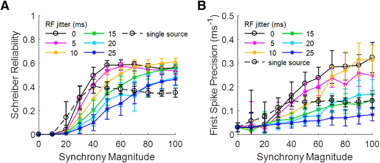
All of the above simulations have assumed that the RF centers for each of the MS LGN inputs was identical relative to the phase of the drifting sine wave grating along the axis of preferred orientation. We conducted further simulations with temporal shifts of the LGN input spike trains to represent the RF phase jitter of V1 simple cell synapses, not all of which are aligned with the orientation of the visual stimulus (Stanley et al., 2012). The amount of temporal shift added to each group of LGN synapses (i.e., to each LGN axon) was randomly selected from a normal distribution with SD (RF phase jitter) from 5 to 25 ms in 5-ms steps, and it remained constant for a given axon for all 30 trials in a given set (see Materials and Methods). Figure 6A,B illustrates the impact of RF phase jitter on reliability and first-spike precision, respectively. The addition of RF jitter primarily serves to make reliability plateau at higher SMs than in the MS case with all RFs aligned, while first-spike precision dramatically worsens for all SMs when jitter rises above 10 ms.

Effects of input spike train alignment on output reliability and precision. (Spike trains vary from trial to trial.) A, B, Introducing RF jitter among LGN input sources causes inter-trial reliability to plateau later and reduces precision of first spike times. Note that 0-ms RF jitter is equivalent to MS input from previously in the article and that RF jitter does not apply to SS input. All error bars represent SD across 25 trial sets.
Figure 6 confirms that in all cases, both for reliability and precision, the MS connectivity between LGN and V1, with its intra-trial variability, is statistically superior to single-source connectivity, with its perfect intra-trial synchrony, even in the presence of RF jitter. However, excessive intra-trial variability is not always beneficial. RF jitter adds another layer of intra-trial variability on top of the intrinsic spiking variability of synchronous LGN cells, which has been explored until now, without affecting inter-trial variability. This puts a limit on the amount of input variability that MS connectivity is able to average out. As the spread in the relative timing of LGN RF activations increases, a greater number of converging synapses (SM) is required to maintain reliable and precise response timing relative to visual events. We will continue to include RF jitter in subsequent figures as we explore the connectivity parameters needed to match experimentally recorded V1 cell output.
Matching simulated output to experimental recordings
In the simulations of Figure 6, we varied both the number of LGN neurons afferent to the V1 cell and the phase jitter among the RFs of these sources over a wide range. The question arises as to what combinations of these two connectivity parameters produce V1 output spike trains from our simulated thalamocortical connectivity system that best match those from the Kara experimental data. We sought to answer this by analyzing a number of models, each with a different combination of RF jitter and SM. Each model used MS connectivity (group size 5) and the same statistical protocol of 25 sets of 30 trials, each set using a unique random axonal configuration (see Materials and Methods). Four measures were used to compare the models. The first two, Schreiber reliability and first-spike precision, come from the connectivity studies above. We added number of spikes per trial and FF, as motivated by the experimental paper (Kara et al., 2000). Although not completely independent, these four measures are distinct characteristics of spike rasters.
We compared the ranges of measurables for each V1 simulation model to those for the experimentally recorded V1 neuron (Kara et al., 2000). The spike trains of one of the recorded V1 cells, labeled LGNA, had the following properties: reliability 0.43 ± 0.05, first spike jitter 9.25 ± 1.84 ms, spike count 2.80 ± 0.27, FF 0.32 ± 0.10. Figure 7A illustrates the spike raster for the experimental V1data (Kara et al., 2000) and for several of the models designated by their SM and their RF jitter. By eye, the model using SM 70 and 15-ms RF jitter seems to best match the experimental raster in terms of numbers of spikes and their distribution in time. (Note that the temporal offset of the rasters of each model is irrelevant to the metrics.)

Multidimensional comparison of simulated V1 model outputs to experimental spike trains. We ran an assay of V1 models that varied in both SM and RF phase jitter, as in Figure 6. A, Output rasters of several example models. Each model ran 25 sets of 30 trials and calculated four measurables (Schreiber reliability, FF, mean spike count/rate, and first spike precision) for each trial set. B, Trial sets as points in two dimensions of measurement space for each of the example models in A. Each cluster contains 25 points, color coded by source model (same colors as in C). Ellipses represent best-fit ellipses to the cluster of points measured from the experimental Kara V1 spike trains (not shown for clarity), analyzed in the same way as the model outputs (red ellipse = 1 SD, blue ellipse = 95th percentile). C, Cumulative plots of sorted r values (normalized eigen-distances in measurement space or number of SDs relative to experimental cluster; see Materials and Methods) of experimental and example model points. D, Heat map of the RMS displacement (dM) between the model and experimental CDFs for all models in the assay. The models whose distribution of measurables most closely matched that of Kara's V1 recordings received between 70 and 90 synaptic inputs (14–18 LGN sources) with a RF phase jitter among LGN sources of 15 ms.
For each model, every set of 30 trials yielded one point in four-dimensional measurement space. With 750 trials, this gave a cluster of 25 points for every model and for the experimental V1 data (selected from the 805 trials labeled B1G by Kara). The most realistic models have the most overlap of their points with the distribution of experimental data. As an example, Figure 7B shows data points in the two-dimensional projection onto FF/Reliability subspace for the same models as in Figure 7A (colored the same as in Fig. 7C). On this projection, the blue dots of the SM 70, 15-ms jitter model tightly cluster within the one SD (red) and 95% confidence (blue) ellipses of the experimental data, more so than the other models. The other five two-dimensional projections of measurement space are constructed in the same fashion (data not shown here).
To quantify similarity of model to experiment, we used a unique metric that considers deviations of model data from experiment in high-dimensional space (see Materials and Methods). We used the covariance matrix of the experimental distribution to transform measurement space into a normalized eigenspace, where distance from the origin, r value, represents the number of SDs from the center of the experimental distribution. All points with the same r value form a hyperellipsoid around the experimental data proportional to its 1-σ best-fit hyperellipsoid. Thus, each model (and the recorded V1 cell) has 25 r values, which can be sorted into a CDF (Fig. 7C). The first curve (black) is for the experimental V1 data (Kara et al., 2000). By taking the RMS deviation (dM) of each model curve from the experimental curve (in Fig. 7C), the degree of dissimilarity between model outputs and V1 recordings can be ascertained as a scalar, where 0 is perfect similarity and larger numbers indicate poor correlation. In Figure 7D, we plot the results for simulations of 63 models over a range of SM and RF jitter values where those models with output spike rasters most like the real V1 recordings have low dM values in bright yellow. The SS case is included for comparison and proves inferior to many of the MS cases.
The 63 models above all used LGN spike trains from a single LGN cell (LGNA) as inputs and compared the simulated trains with the trains from a single V1 cell that was simultaneously recorded in the same experiment (labeled B1G in the data provided by Kara). A similar pattern appears when comparing model output to other recorded V1 cells, even when driven by different LGN inputs (see Materials and Methods). In Figure 8, we repeated the 750 trial simulations for all 63 models using the 12 combinations of the three recorded LGN cells for input and the four recorded V1 cells as comparison based on the same metric comparison protocol as in Figure 7. Only nine of the 12 comparisons are of interest as experimental V1 cell C2B appears to have dissimilar spike trains from the other three (Fig. 8, legend). Note that the heatmap patterns appear to have more similarity across V1 cell comparisons for a given LGN driver than across LGN drivers for a given V1 cell comparison. This hints that afferent spiking patterns have a greater impact on output patterns of activity than does the identity of individual V1 cells. However, a quantitative analysis of this effect is beyond the scope of this article.

Correlations between V1 model thalamocortical connectivity and biophysical realism in V1 output. Heatmaps showing similarity (dM; see Materials and Methods, Multidimensional validation metric) of model V1 neuron output to experimental recordings for all combinations of LGN inputs and V1 outputs (Kara et al., 2000). Model neurons were driven exclusively by LGN spike trains from a single recorded LGN precursor cell (LGNA on row 1, LGNB on row 2, LGNC on row 3). Each column corresponds to the recorded V1 cell from the Kara data to which the model V1 cell's output was compared (labels derived from the filename used for each anesthetized cat). Green boxes highlight those cases where both the driving LGN cell and the compared V1 cell were recorded in the same experiment. As in Figure 7D, the rows of each heatmap correspond to the RF phase jitter applied between LGN sources (ms), and the columns denote SM (total number of synapses). Except for SS, all inputs used a group size of five synapses per source axon. Blue corresponds to poor agreement with experiment (high dM) and yellow to good agreement (low dM). Note how the clustering of good model parameters changes markedly when comparing model outputs to V1 cell C2B relative to the other V1 cells, suggesting that cortical cell C2B differed in some significant way.
Good matches between models and recordings appear to be consistent in the range of SM 60–90 synapses and RF jitter 15–30 ms. In particular, the combination of SM 70 synapses and RF jitter 15 ms is close to the best case in all nine comparisons. Thus, this analysis suggests that the best fits are for models having an RF jitter around 15 ms and SM between 70 and 90 synapses, corresponding to 14–18 LGN sources (i.e., MS connectivity). The match for the optimal model parameters for this set of four measurements is remarkably close to the experimental data, even without adjusting the many free parameters in the NEURON model of the V1 spiny stellate cell.
Quantitative analysis of MS connectivity improvement
To demonstrate that the advantage of intra-trial variation (MS) over synchrony (SS) is model independent, and therefore generally applicable, we cross-validated with both artificially generated LGN spike trains and simplified neural models (Izhikevich and integrate-and-fire) using the same experimental LGN spike trains (Kara et al., 2000) for inputs as used with the NEURON model and the same simulation protocol of 750 trials in sets of 30 (see Materials and Methods, Model independence). Figure 9C,E shows that there is a significant reliability improvement for MS at all SMs above 20 for both an integrate-and-fire model neuron (Stanley et al., 2012) and a somewhat more realistic Izhikevich model (Izhikevich, 2003), respectively. These model V1 neurons have deterministic synapses, which produce a release (and EPSC) for every spike, and receive no random background stimulation, which avoids noisy fluctuations in their membrane potentials. To control for effects specific to the experimental LGN spike trains, artificial input spike trains with Gaussian distributions were also used. Even with artificial input spike trains, reliability still increased with SM in almost exactly the same fashion as with experimental inputs. These same general trends, both of the increase of reliability with total number of synapses and the greater V1 output reliability with MS LGN input rather than SS, follow the patterns seen for the NEURON model, using both natural and artificial LGN spike train inputs (Fig. 9A).

Model independence of observed trends that inter-trial reliability improves with number of LGN sources. A, C, E, Schreiber reliability trends for NEURON, Izhikevich, and integrate-and-fire neuron models, comparing outputs that used experimentally recorded LGN input with those that used artificial input (see Materials and Methods, Model independence). MS LGN input produced more reliable output than SS for all three neuron models and for both artificial and real LGN input [significant improvement (p < 0.01, Welch t test, n = 25) for SM ≥ 40 (NEURON, LGN), SM ≥ 50 (NEURON, artificial), SM ≥ 20 (Izhikevich, both), and SM ≥ 30 (integrate-and-fire, both)]. B, D, F, Comparison of theoretical to observed ratios in first spike time jitter between MS and SS as a function of number of LGN sources for each V1 neural model. SM held constant at 60 total thalamocortical synapses for all data. As neuron dynamics become more mathematically abstracted from physiology (from NEURON to Izhikevich and from Izhikevich to integrate-and-fire), the observed trends in MS to SS jitter ratio better fit the theoretical  curve (R2 = −1.019 for NEURON with background noise, R2 = 0.535 for NEURON without background noise, R2 = 0.659 for Izhikevich, R2 = 0.889 for integrate-and-fire). Intrinsic model noise from best-fit a + (1 − a)/
 trend (horizontal asymptote) also decreased with increased distance from physiological realism: a = 0.500 for NEURON with background noise (R2 = 0.354), a = 0.194 for NEURON without background noise (R2 = 0.760), a = 0.152 for Izhikevich (R2 = 0.778), a = 0.041 for integrate-and-fire (R2 = 0.899). [Background noise in NEURON model arises from the 5600 intra-cortical synapses in the V1 model neuron (Fig. 1) and from the stochastic excitatory synapses.] All error bars represent SD across 25 trial sets.
The explanation for this model-independent phenomenon comes from statistics. Assuming that the first spike estimates the timing of a visual stimulus and assuming that LGN cells independently estimate timing with a variance of σ2 (∼[7 ms]2 here), an idealized V1 cell that samples n LGN spike trains should have a SEM estimated time of  , purely based on statistical considerations (Everitt and Skrondal, 2010; Jeanne and Wilson, 2015).
To test how well this theory matches our results, we analyzed the ratio in first-spike time jitter between the V1 output of models receiving MS and SS input (Fig. 9). (The term “first-spike time jitter,” which is the inverse of first-spike time precision used heretofore, was employed in the analysis of Fig. 9 for convenience. Note that the ratios in these figures do not change for either terminology.) We controlled for total input strength by fixing SM at 60, changing the number of sources between MS models [n (a factor of 60) LGN sources, group sizes of 60/n synapses per source axon]. First-spike time jitter was calculated for 25 sets of 30 trials per model, and MS:SS jitter ratios were calculated for all 625 comparisons between model trial sets.
As shown in Figure 9D,F, without the complexities of the biophysically based V1 neuron, the precision improvement curve for idealized neurons closely matches that of the theoretical  curve (dashed red line). However, for the more biophysical NEURON model, the MS:SS first-spike jitter ratio (Fig. 9B, solid black line) does not improve as much as the theory predicts. The curve plateaus higher than the theoretical
  improvement (a = 0.500, see Eq. 7 in Materials and Methods), which we hypothesized is due to input noise sources in our model, such as background cortical spiking (the 5600 intra-cortical synapses in the V1 model neuron shown in Fig. 1) and stochastic synapses. With these two noise sources removed (dotted blue curve), in the same way as in the idealized neuron models, the precision ratio curve again approaches that of the theoretical, plateauing much closer to 0 (a = 0.194).
In summary, the  improvement factor for multiple LGN sources is not at all due to complexities in our biophysical V1 model nor to the biophysically generated spike trains from drifting grating stimuli. It is, in fact, a general property of interconnected spiking neurons that use jittered synchronous spike trains to carry information.
Synchrony and connectivity
We further studied the effects of varying connectivity over a wide variety of LGN cell numbers and synaptic group sizes. For this analysis, we withheld RF jitter to isolate the effects of the synapse and LGN source numbers.
The heat map in Figure 10A shows the Schreiber reliability for V1 cells with different numbers of LGN afferent cells and of synapses per source (1–15 for each), averaged from 10 sets of 30 trials each. Hyperbolas of constant SM (the number of LGN cells times the number of synapses per cell) overlay the heat map with a gray box around simulations with a group size of five synapses per LGN, which has been used for most of this article. Figure 10B shows the same reliabilities divided by the corresponding SMs, revealing a tradeoff between spike timing reliability and the efficiency of synaptic resource utilization. The strongest reliability payoff for adding synapses occurs between SM 30–50, with diminishing returns on reliability improvements for SMs after ∼70–90 synapses. This 70–90 synapse range agrees with the best fit range of SMs estimated in Figure 8 for neurons recorded from cat visual cortex. It therefore appears that these neurons are striking a balance between energy constraints, which would tend to minimize the number of synapses in the visual pathway, with the need for precise visual timing information, which would seek to maximize them. Future investigations would benefit from exploring this information-energy tradeoff.

Heat maps showing inter-trial reliability of V1 neuron outputs for an assay of models with varying numbers of LGN sources and synapses per source. Hyperbolas of constant SM (number of sources times group size per source) are shown for clarity. Gray box encloses models with a group size of five synapses per source, used for most of the article. Values represent the average measure from 10 sets of 30 trials. All models use zero RF jitter between sources. A, Schreiber reliability as a function of number of LGN sources and synaptic group size. Note how reliability improves with SM. B, Schreiber reliability divided by SM of the model. Adding thalamocortical synapses yields diminishing returns after about SM = 50.
Thus, it seems that for this investigation, based on the anesthetized cat and moving grating stimulation, realistic reliability involves LGN inputs having ∼5–10 synapses per axon, in agreement with anatomical data (da Costa and Martin, 2009, 2011). In addition, at least seven LGN cells should be synchronously activated to optimize reliability of the outputs for a minimum number of synapses, balancing timing information with energy load. The apparent relationship between group size and the number of sources means that maintaining a fixed reliability value when increasing group size requires a simultaneous decrease in SM and vice versa.
While this article focused on the effect of converging inputs on event-response timing reliability for single neurons between trials, we expect that the same principles would probably apply for timing reliability among multiple cortical neurons in the same trial. With overlapping RFs, multiple cortical neurons could have access to the same timing information on each trial, and the jitter in response timing among them should theoretically fall as  with the number of LGN inputs, at least insofar as the intra-trial variation in LGN spike timing follows the inter-trial variation. Synchrony among cortical cells in the same trial may be important for generating a robust response to time-sensitive visual stimuli. However, these considerations are outside the scope of this article.
Discussion
Based on experimental recordings from the anesthetized cat, we have uncovered the effects of LGN input synchrony and spike train variability, both within and between trials, on the reliability and timing precision of firing patterns in spiny stellate neurons from the V1 cortex. The number of LGN input sources (afferents), the number of synapses per afferent, and the total number of LGN synapses on the V1 neuron directly affected the reliability and timing precision of the V1 spike trains in our model (Fig. 10). There are also preferred combinations of these numbers that produce model V1 spike trains statistically similar to those from cat V1 experiments (Fig. 8). These optimal combinations are in broad agreement with the literature on LGN to V1 connectivity and RF structure (Hubel and Wiesel, 1962; Alonso et al., 2001; da Costa and Martin, 2009, 2011; Stanley et al., 2012). This adds a new mechanism to the literature by which cortical neurons in the primary visual pathway of mammals are able to reliably report timing of visual stimuli (Mainen and Sejnowski, 1995; Haider et al., 2010).
Synaptic input from multiple LGN axons leads to improved reliability and precision
By modeling each dendritic synapse on the V1 neuron individually, it was possible to study the effects of LGN input variability with different thalamocortical connectivity configurations. This revealed that individual V1 neuron event timing, as measured by both reliability and first spike time precision in our model, is degraded by LGN inter-trial variability alone to a point below that needed in vivo (Kara et al., 2000). However, increasing the intra-trial input variability via more LGN afferents, each with a different spike train pattern, improved the reliability and timing precision of the V1 output spike trains to the range found in vivo. In Figure 4, for example, at a total LGN synapse count (i.e., SM) of 60, both the V1 output raster reliability and the first-spike jitter are significantly improved (from 0.4 to 0.6, and 7.7 to 4.2 ms, respectively) with intra-trial variability introduced by 12 LGN cells, each having 5 synapses on its axon. Furthermore, timing precision continues to improve with more independent LGN precursor cells (Fig. 9).
In addition, we confirmed that the improvement in mean event time jitter of the V1 neuron dropped with the square root of the number of synchronous LGN input sources following theory for idealized neurons such as the leaky integrate-and-fire (Fig. 9). As the model neuron becomes more realistic, it deviates from this ideal trend due to noise sources within the model (Fig. 9) but is still significant. Direct measurements of LGN axon synapses on spiny stellate cell dendrites confirm this configuration as realistic with a broad average around five synapses per axon per cell, mostly on separate dendritic branches (Peters and Payne, 1993; Alonso et al., 2001; da Costa and Martin, 2011).
Similar results for the effects of presynaptic neuron convergence on spike timing have been reported for in vitro slices from rat auditory cortex (Xu-Friedman and Regehr, 2005a,b) and in the olfactory system of Drosophila (Jeanne and Wilson, 2015). There are also several studies on the effects of trial-to-trial and intra-trial variability on temporal precision in the cat visual pathway (Alonso et al., 1996; Kumbhani et al., 2007; Desbordes et al., 2008, 2010; Herikstad et al., 2011).
Model output spike train rasters are consistent with experiments
We introduced a scalar metric for quantitatively matching the recorded Kara V1 spike rasters to the model V1 spike rasters based on four statistical measures: Schreiber reliability, first spike precision, FF, and spike count per trial. Without changing any parameters of the V1 cell computational model, a close match was obtained for SM between 70 and 90 total synapses (with group size 5) and RF jitter of ∼15 ms (Fig. 7). This range was little changed for simulations driven by spike trains from any of three recorded LGN cells and compared to the rasters of any of three recorded V1 simple cells (Fig. 8). There is also a tradeoff between the information retention (i.e., event timing) in V1 and the energy requirements due to the number of synapses as suggested by Figure 10 which compares V1 output reliability over a range of values for the three synaptic connectivity parameters. Future work is indicated to compare the effects of other parameters in this model using additional measures of comparison between model and in vivo experiments, such as intra-spike timing.
Robustness of the V1 model and generality of the results
The detailed V1 spiny stellate cell model used in this study was shown to produce results directly relatable to in vivo mammal experiments. However, changes to our model or to experimental conditions can be expected to change our results. For example, it is now well established that awake behaving animals (Gur et al., 1997; Niell and Stryker, 2010), natural intensity lighting (Farrow et al., 2013), and natural scene stimulation (Herikstad et al., 2011; Baudot et al., 2013) change the behavior and physiological responses of neurons in the V1. These changes can manifest as dramatic differences in the fluctuations of spike trains (Gur et al., 1997; Gur and Snodderly, 2006), in synaptic mechanisms (Xu et al., 2012), and in intrinsic mechanisms of the spiny stellate cell itself.
The parameter values for the excitatory synapses in the V1 cell model were selected to mimic the timing of release trains measured in vitro (see Materials and Methods). More recent experiments in the live cat (Boudreau and Ferster, 2005) provide evidence that in vivo depression might be much more saturated during a trial than in our model. However, we do not expect this to impact our results and conclusions significantly. In fact, for all cases in Figure 9 where synaptic depression was removed (the no noise NEURON model and both the Izhikevich and integrate-and-fire models), the results matched the theoretically expected  trend even more precisely than when our depression-heavy synaptic model was included. The improvement in reliability and precision from adding more input sources results directly from fundamental laws of statistics and is robust to qualitative changes to the model that do not impact the assumptions of source independence.
There is also experimental evidence for ∼30 separate presynaptic LGN neurons per V1 cortical neuron (Reid and Usrey, 2004). This would lead to a total number of V1 synapses of 30–150 or even more, depending on the synapse group size. Although our study focused on the range of 20 or fewer LGN synapses and 100 or fewer synapses, our basic conclusions as to the effects of inter-trial and intra-trial variability, as well as the ranges of the connectivity parameters, should remain valid at 30 LGNs.
Another limitation in this study is that we used recorded LGN spike trains from a limited set of experiments and we used the multiple trials of a single neuron for intra trial variability for some of our results. Figure 4 indicates that, at least for three different recorded LGN cells, our major results for a difference with and without input variability remain significant.
Implications for spike timing and synchrony in the neural code
There is evidence that microsaccades of the eyes during and between trials (Gur et al., 1997; Gur and Snodderly, 2006) could be a cause of LGN spike train variability (Fig. 2). Thus, the variability should not be considered “noise” but may be, in fact, part of the neural code. Variability is affected by rapid spatiotemporal RF changes interacting with the moving visual stimulus. On a somewhat slower time scale, our model used random RF jitter to emulate this effect, reliably evoking a V1 first spike with a SD of <10 ms, much narrower than the 150-ms input spike train. This suggests a neural code based on spike timing (Bialek et al., 1991) in which this first spike can reliably convey the information that a visual stimulus has appeared on the retina within its RF (Butts et al., 2010). Such a code would be sparse (Olshausen and Field, 2004) and consistent with the classical simple cell RF model (Hubel and Wiesel, 1962). This is also appealing since spike timing has been observed to have less variability than spike count in cat V1 responding to natural movie stimuli (Herikstad et al., 2011).
Our results are also consistent with a synchrony code (Stanley, 2013) where coordinated activity within a population (Zandvakili and Kohn, 2015) determines the communication paths for conveying and processing information (Brette, 2012) in cortical networks. This concept is based on experimental and modeling evidence that synchronous thalamic inputs (on the order of 10 ms) are effective in driving single cortical targets even when synapses are weak (Alonso et al., 1996; Bruno and Sakmann, 2006). Thus, MS synchrony likely serves as a factor in transferring information throughout other parts of the visual pathway and cortex.
Footnotes
- Received November 3, 2017.
- Revision received March 26, 2019.
- Accepted May 10, 2019.
*H.-P.W. and J.W.G. and co-first authors.
The authors declare no competing financial interests.
This work was supported by the Howard Hughes Medical Institute. We thank Prakash Kara and R. Clay Reid for providing their in vivo visual pathway recordings in the cat. Our results arose from careful examination and analysis of these simultaneously recorded retinal, LGN, and V1 responses. Also, we thank Jean-Marc Fellous, who originated this project and wrote much of the comprehensive simulation code.
- Correspondence should be addressed to Terrence J. Sejnowski at terry{at}salk.edu
- Copyright © 2019 the authors