


Abstract
We studied orientation selectivity in V1 of alert monkeys and its relationship to other physiological parameters and to anatomical organization. Single neurons were stimulated with drifting bars or with sinusoidal gratings while compensating for eye position. Orientation selectivity based on spike counts was quantified by circular variance and by the bandwidth of the orientation tuning curve. The circular variance distribution was bimodal, suggesting groups with low and with high selectivity. Orientation selectivity was clearly correlated with spontaneous activity, classical receptive field (CRF) size and the strength of surround suppression. Laminar distributions of neuronal properties were distinct. Neurons in the output layers 2/3, 4B and 5 had low spontaneous activity, small CRFs and high orientation selectivity, while the input layers had greater diversity. Direction-selective cells were among the neurons most selective for orientation and most had small CRFs. A narrow band of direction- and orientation-selective cells with small CRFs was located in the middle of layer 4C, indicating appearance of very selective cells at an early stage of cortical processing. We suggest that these results reflect interactions between excitatory and inhibitory mechanisms specific to each sublamina. Regions with less inhibition have higher spontaneous activity, larger CRFs and broader orientation tuning. Where inhibition is stronger, spontaneous activity almost disappears, CRFs shrink, and orientation selectivity is high.
Introduction
Orientation selectivity is of prime importance to the brain's ability to analyze the visual scene. The organization of V1 into orientation columns is evidence of the functional importance of this feature (Hubel and Wiesel, 1968, 1974). Within an orientation column, cells share a similar preferred orientation, but they have diverse physiological properties, one of the most dramatic being direction selectivity. Given the intricate anatomy within an orientation column, we have explored how orientation selectivity is associated with other physiological characteristics and how it is related to the laminar location of the cell.
Extensive qualitative evidence shows that cells weakly selective for orientation tend to be spontaneously active, and that the level of spontaneous activity and the level of orientation selectivity covary throughout the orientation column. Many authors agree that in layer 4C, orientation selectivity is weak; this is particularly evident in layer 4Cβ where most cells lack orientation selectivity (Poggio et al., 1977; Bauer et al, 1980; Bullier and Henry, 1980; Dow et al., 1981; Blasdel and Fitzpatrick, 1984; Hawken and Parker, 1984; Livingstone and Hubel, 1984; Leventhal et al., 1995; Snodderly and Gur, 1995). Most authors also find that 4Cβ cells display a high level of spontaneous activity (Poggio et al., 1977; Bauer et al., 1980; Livingstone and Hubel, 1984; Snodderly and Gur, 1995). Similar to layer 4Cβ, cells in Layer 4A are not very selective for orientation (Poggio et al., 1977; Blasdel and Fitzpatrick, 1984; Snodderly and Gur, 1995), and are spontaneously active (Poggio et al., 1977; Snodderly and Gur, 1995) while cells in layers 2/3, 4B and 5 are highly selective and have a low level of spontaneous activity (Poggio et al., 1977; Bauer et al., 1980; Blasdel and Fitzpatrick, 1984; Hawken and Parker, 1984; Livingstone and Hubel, 1984; Snodderly and Gur, 1995).
Contrary to the classical view, Ringach and colleagues (Ringach et al., 2002b) recently concluded from quantitative measurements that orientation selectivity in V1 of anesthetized monkeys is almost uniformly distributed, as assessed both by physiological measures and laminar distributions. These results have led to the proposal that V1 should be considered a diverse, but relatively unspecialized, cortical region (Shapley et al., 2003).
We have studied orientation selectivity and its relationship to other physiological features in V1 of alert monkeys, where the potential confounding effects of anesthesia are eliminated. Our quantitative data support the concept of great diversity in orientation selectivity of cells in macaque V1, but they also show that the distribution of orientation tuning is nonuniform. Furthermore, the laminar distribution of orientation selectivity is highly differentiated. Our results suggest that both the diversity of orientation tuning and the intricate laminar distribution result from organization into parallel specialized processes that are precisely linked to later cortical areas.
Materials and Methods
Six adult female monkeys (two Macaca fascicularis and four M. mulatta) were used. Monkeys were trained to fixate on a light-emitting diode (LED) for water reward. Once the monkey learned the task, a head-holding post and a recording well were implanted under deep anesthesia. All procedures complied with National Institutes of Health guidelines and were approved by the Animal Care and Use Committee of the Schepens Eye Research Institute.
Nerve-spike and eye-movement recording
Fiber electrodes made from quartz-insulated platinum–tungsten alloy (Eckhorn and Thomas, 1993) with bare tip lengths ≤5 μm and impedance at 1 kHz of 3–4 MΩ were most frequently used to record single-unit activity. In some experiments, glass-insulated platinum–iridium electrodes (Snodderly, 1973) with a tip diameter of 1–1.5 μm, and bare tip length of 5–7 μm, were used. Cells were assigned to cortical layers based on histological and/or physiological criteria as previously described (Snodderly and Gur, 1995; see below). In the initial experiments, position of the dominant eye was monitored by a double Purkinje image eye tracker (2–3 minarc resolution; 100 Hz sampling rate) and recorded in a computer file, together with spike arrival times (0.1 ms time resolution) and spike shapes collected at 10–25 kHz (Gur et al., 1999). In recent experiments, eye position was recorded with an implanted scleral coil (Robinson, 1963; Judge et al., 1980a; 1–2 minarc resolution; 200 Hz sampling rate). The trial started when the monkey correctly pressed the lever in response to the LED and continued for 5 s provided that the gaze remained within a predefined fixation window, between ±0.5° and ±1.5°.
Stimulus Presentation
In the initial experiments, bar and grating stimuli were displayed on a Barco 7351 monitor at a 60 Hz noninterlaced frame rate, with a Truevision ATVista video graphics adapter. In recent experiments, stimuli were displayed on Sony 500 PS monitor at a 160 Hz noninterlaced frame rate with a Cambridge Research Systems VSG2/3F video board. Bars were optimized for orientation, length, velocity and color (green or red), 0.9 or 1 log units brighter or darker than the background of 1 or 5 cd/m2. This luminance is in the low photopic range and stimuli are vividly colored. Chromatic stimuli were generated by activation of individual guns of the monitor. Incremental (bright) bars were presented on a neutral gray background; decremental (dark) bars were presented on a background of a single color (Snodderly and Gur, 1995). Monochrome sine gratings of 50% luminance contrast, optimal orientation, length and color were presented on backgrounds of the same color as the decrement bars, with a mean luminance of 1 or 5 cd/m2. Gratings had the same mean luminance as the background or were presented so that the maximal luminance corresponded to the luminance of the increment bar. After the ocular dominance was established, stimuli were viewed binocularly, unless responses during monocular viewing were substantially stronger. The eye position signal was added to the stimulus position signal at the beginning of each video frame (bars) or in the early experiments with gratings, each second frame (‘image stabilization’, Snodderly and Gur, 1995; Gur and Snodderly, 1987, 1997a,b). This was done to compensate for changes in eye position during intersaccadic intervals. Note that the maximum delay between shifts in eye position and subsequent corrections could be as long as 28 ms for bars and 44 ms for gratings for the 60 Hz frame rate, and 10 ms for both types of stimuli at the 160 Hz frame rate; thus this procedure was not intended to compensate for the fast saccadic eye movements. Saccades were automatically detected using a stability criterion combined with a velocity threshold of 10°/s (Snodderly et al., 2001), and responses occurring within ∼100 ms of a saccade were excluded during data analysis so that all data were collected only during inter-saccadic drift periods. Changes in eye position during drifts were typically <10′/s (Fig. 1A) so that even the largest delay (28 ms) in eye position compensation would have caused an insignificant position error (<0.3′). Using this approach enabled us to accurately map receptive fields (Snodderly and Gur, 1995; Kagan et al., 2002) and to produce consistent measures of neuronal responses (Gur et al., 1997) in alert monkeys.
![Comparison of physiological characteristics of a cell weakly selective for orientation (left column) and a highly selective cell (right column). The horizontal axis represents time in milliseconds for sections (A)–(C), and tilt in degrees for (D), with the peak of the orientation tuning curve shifted to a nominal 90° for purposes of illustration. (A) Examples of behavioral trials of 5 s duration. Eye position (thick line = vertical; thin line = horizontal) is plotted along with the spike train (short vertical lines under the eye position traces). First two rows: (1) optimal and (2) suboptimal orientations. A bar was swept forward and back across the receptive field for several cycles. The time periods of the sweeps in one direction are indicated by the thick lines on the horizontal axis. Responses evoked by the preferred direction of stimulus motion during the intersaccadic drift periods (rectangles) curves were automatically selected and used for calculating the tuning curve. Responses occurring within ∼100 ms of a blink (e.g. left column, second row; ∼1800 ms) or a saccade (e.g. right column, first row, ∼1700 ms) were excluded during data analysis so that all data were collected only during inter-saccadic, drift periods. This monkey had a slow, systematic vertical drift during maintained fixation, which is a common pattern among monkeys (cf. Fig. 1 of Gur and Snodderly, 1997a). The third row (3) shows ongoing activity during trials where the monkey was viewing a blank screen, segmented according to sweep cycle duration in stimulation trials. (B) Raster displays of several individual responses are shown above peristimulus time histograms fitted with a Gaussian function for the optimal orientation (1), a suboptimal orientation (2) and ongoing activity segments from trials with a blank field (3, ong.). Spikes outside ±3 SD of the peak of the Gaussian function were considered to be due to ongoing activity during the stimulus trial. The mean ongoing rate was estimated and the expected number of ‘ongoing spikes’ within the response period was subtracted from the spike count of the evoked response. Note that while the ongoing firing rates during presentation of a blank field for the spontaneously active cell [A, (3), left panel] was 23 spikes/s, the mean ‘ongoing’ rate of the same cell between evoked responses in the sweeping bar trials [A, (1), (2), left panels] was only 16 spikes/s. (C) Estimation of activating region (AR) width. Gray line = the cumulative curve; dashed vertical lines = intersections of least-squares lines fitted to the cumulative curve. AR borders were defined by 95% of the response between the intersections, distributed symmetrically around the center of mass (not shown). (D) Resulting orientation tuning curves. Open circles = data points; solid lines = curves interpolated and smoothed as described in Materials and Methods. Black line = no subtraction of the ongoing activity (each point represents the mean spike count during a total sweep duration); gray line = after subtraction of estimated contribution of ongoing activity during the response period, as described in (B). For the silent cell in the right column the two tuning curves are identical.](https://oup.silverchair-cdn.com/oup/backfile/Content_public/Journal/cercor/15/8/10.1093/cercor/bhi003/2/m_cercorbhi003f01_ht.jpeg?Expires=1716372050&Signature=YI7BHkPPeBYKR3k~VTy0jWB0p7IkfotLihHiJtkObqOgobpxogZ5G3rDADa6DnNga7setkHzGk5XAMx0aWRtWdIH6J~42WX-8yKkTixmzCbTnOaD3EtsLFQlzgGnKgf3zxtbgq4Kn5Gp0rW9UQJrPcN69j6kuGWmshk3a8TbBlxIsZX2gdwWmzjCUbT6p2zvDvb8Ok~SUWkxAsJDM7L--jSsUzyK8YurB0yCGCgnPFJ2LOHVl-a8q-G~xnFKZTwR4TrOGt8t9hbKbd004lBVcrn4FDKGI~dgpTzhy6zu5Go5~IAUWuO9CqFvZTbjRJofmiIYz2y-TwXXDjxm5mRR1Q__&Key-Pair-Id=APKAIE5G5CRDK6RD3PGA)
Comparison of physiological characteristics of a cell weakly selective for orientation (left column) and a highly selective cell (right column). The horizontal axis represents time in milliseconds for sections (A)–(C), and tilt in degrees for (D), with the peak of the orientation tuning curve shifted to a nominal 90° for purposes of illustration. (A) Examples of behavioral trials of 5 s duration. Eye position (thick line = vertical; thin line = horizontal) is plotted along with the spike train (short vertical lines under the eye position traces). First two rows: (1) optimal and (2) suboptimal orientations. A bar was swept forward and back across the receptive field for several cycles. The time periods of the sweeps in one direction are indicated by the thick lines on the horizontal axis. Responses evoked by the preferred direction of stimulus motion during the intersaccadic drift periods (rectangles) curves were automatically selected and used for calculating the tuning curve. Responses occurring within ∼100 ms of a blink (e.g. left column, second row; ∼1800 ms) or a saccade (e.g. right column, first row, ∼1700 ms) were excluded during data analysis so that all data were collected only during inter-saccadic, drift periods. This monkey had a slow, systematic vertical drift during maintained fixation, which is a common pattern among monkeys (cf. Fig. 1 of Gur and Snodderly, 1997a). The third row (3) shows ongoing activity during trials where the monkey was viewing a blank screen, segmented according to sweep cycle duration in stimulation trials. (B) Raster displays of several individual responses are shown above peristimulus time histograms fitted with a Gaussian function for the optimal orientation (1), a suboptimal orientation (2) and ongoing activity segments from trials with a blank field (3, ong.). Spikes outside ±3 SD of the peak of the Gaussian function were considered to be due to ongoing activity during the stimulus trial. The mean ongoing rate was estimated and the expected number of ‘ongoing spikes’ within the response period was subtracted from the spike count of the evoked response. Note that while the ongoing firing rates during presentation of a blank field for the spontaneously active cell [A, (3), left panel] was 23 spikes/s, the mean ‘ongoing’ rate of the same cell between evoked responses in the sweeping bar trials [A, (1), (2), left panels] was only 16 spikes/s. (C) Estimation of activating region (AR) width. Gray line = the cumulative curve; dashed vertical lines = intersections of least-squares lines fitted to the cumulative curve. AR borders were defined by 95% of the response between the intersections, distributed symmetrically around the center of mass (not shown). (D) Resulting orientation tuning curves. Open circles = data points; solid lines = curves interpolated and smoothed as described in Materials and Methods. Black line = no subtraction of the ongoing activity (each point represents the mean spike count during a total sweep duration); gray line = after subtraction of estimated contribution of ongoing activity during the response period, as described in (B). For the silent cell in the right column the two tuning curves are identical.
Receptive Field Mapping
The width and location of receptive-field activating regions (ARs) were estimated with increment (Inc) and decrement (Dec) bars (2–16 minarc, mean 7 ± 3 minarc) swept forward and back at 1.5–7°/s across the receptive field in a direction orthogonal to the optimal orientation axis (Pettigrew et al., 1968; Schiller et al., 1976a; Foster et al., 1985; Snodderly and Gur, 1995; Kagan et al., 2002). During each trial several responses were usually recorded (Fig. 1A). The operational term ‘activating region’ is used to distinguish regions that respond to direct stimulation from other (covert) zones that may modify the directly evoked response (e.g. side inhibition or facilitation from subthreshold regions). The bar width was adjusted to generate strong responses and was typically smaller than the AR width for both RF mapping and derivation of orientation tuning. To optimize the precision of measurement and minimize possible effects of response latency, we calculated AR widths using the lowest velocity that elicited a strong response in the data set for each cell.
Using eye position compensation and appropriate eye movement corrections, average peristimulus time histograms (PSTH) of responses were constructed, and a cumulative curve was superimposed (Fig. 1C; see also Kagan et al., 2002). The cumulative curve was manually divided into three ‘quasi-linear’ sections by selecting the two points where the cumulative curve most rapidly changed slope. The optimal least-squares lines were then automatically fitted to each of the three sections. The AR width was measured as 95% of the region defined by intersections of the three least-squares lines for the response to motion in the preferred direction. If the overall fit was judged to be suboptimal, the selection of the borders between three sections was slightly readjusted. This was done in <20% of the cells and the resulting change in AR estimate was ±10%. As a control for potential bias in this interactive method, a completely unsupervised procedure that minimized the sum of residuals for three-piecewise linear fits across all combinations of intersection points and line slopes was performed on a subset of 150 cells. The correlation between the interactive method and the unsupervised one was very high (r = 0.93, P < 0.0001), and the mean difference between the visually guided estimate and the fully automated one was only 4′ ± 8′ with the mean of the visually guided estimates being slightly smaller.
To distinguish between complex and simple cells, an overlap index (OI) was calculated (Schiller et al., 1976a; Kagan et al., 2002). This ranged from negative values for spatially separated Inc and Dec ARs to 1 for complete and symmetric overlap. All cells with OI ≤0.3 were considered simple, while cells with OI ≥0.5 were considered complex. The total extent of Inc and Dec ARs was considered the classical receptive field (CRF). Mean AR was defined as the average width of all ARs in the receptive field. No cells with >2 ARs are included in the present sample.
A directionality index (DI) was computed as 1 minus the ratio of the response in the nonpreferred direction to the response in the preferred direction. We classified cells as direction selective when their DI was ≥0.5 (Snodderly and Gur, 1995, and references therein). When data were available for both signs of contrast, the mean DI for the two conditions was used for analyses. Reported values of OI were estimated using the preferred direction.
Modulation Ratio
The relative modulation (RM) (DeValois et al., 1982; Skottun et al., 1991) of the response to drifting sinusoidal gratings was calculated as RM = F1/F0, where F0 is the mean firing rate (DC) of the response and F1 the magnitude of the fundamental (first) harmonic of the response, corresponding to the temporal frequency of the grating (usually 5 Hz). The spatial frequency and window size of the stimulus were varied to find the condition that produced the largest values of F1 and of F0, and RM was calculated for the stimulus combination that generated the largest value of the entire set of these two harmonics, which could be either F0 or F1. In addition, RM was calculated for the stimulus condition producing the maximal modulation if that differed from the condition producing the largest F1 or F0 (Kagan et al., 2002). To be consistent with a recent study (Ringach et al., 2002b) we did not subtract the ongoing activity from the grating-evoked responses.
Orientation Tuning: Circular Variance and Bandwidth
Most of our orientation data were collected with drifting bars that changed in orientation in 10–20° angular steps, ranging from 0° to 180° (zero being ‘horizontal’). In addition, for some very narrowly tuned cells we used finer steps around the preferred orientation. Tuning curves were based on number of spikes generated by each sweep minus the ongoing activity (see below). Several responses were averaged for each datum. The curves were linearly interpolated with a 1° step and smoothed with a Hanning filter with a 7° half-width at half-height (Fig. 1D). For a few extremely narrowly tuned cells, a filter with a 5° half-width was used.
The ongoing activity was measured in two ways. For comparison with other physiological properties and to establish the distribution across layers, the activity was measured during trials with a blank screen, uniformly illuminated at 1 or 5 cd/m2 (Fig. 1A, third row).
For many cells the ongoing activity during trials with repeated stimuli was suppressed during the ‘interstimulus’ interval, when the bar was outside the AR (Fig. 1A–C, left column). This suppression was quantified for a subset of 39 cells with >25 spikes/s ongoing rate during trials with a blank screen. It was found that the ongoing activity during interstimulus intervals of stimulation trials was significantly lower than ongoing activity that occurred during trials with only a blank screen (P < 0.01, Wilcoxon matched-pairs test; mean difference 8 spikes/s). To estimate the contribution of ongoing activity to the evoked responses, for each stimulus orientation the mean firing rate in periods outside the evoked response was calculated, and the number of spikes expected during the time period containing the evoked response was subtracted from the response spike count. This procedure is illustrated in Figure 1B and described in the legend.
For comparison with the quantitative data of Ringach et al. (2002b), orientation tuning curves were also calculated without subtracting the ongoing activity. These data are only utilized in Figure 13.
The tuning curve half-bandwidth (HBW) at 1/(21/2) (Ringach et al., 2002b; Schiller et al., 1976b) was calculated directly from the smoothed curves as half the difference between the orientations flanking the preferred orientation at 1/(21/2) peak response. If the tuning curve never went below 1/(21/2) of the peak, the half-bandwidth was defined as 90°.
Assignment to Layers
From our total sample of 339 cells it was possible to assign 170 cells to the various V1 laminae. In the alert preparation it is not possible to use electrolytic lesions as anatomical markers since such lesions are only detectable for a few days. As detailed in Snodderly and Gur (1995; see also Poggio et al., 1977), we used information from several sources to locate the layer of origin: (i) distance from the cortical surface; (ii) physiological properties — an alternating sequence of layers with high ongoing multiunit background activity (4A, 4C and 6), and layers with very low background activity, (2/3, 4B and 5), in addition to the clusters of direction-selective cells found in layer 4B (Livingstone and Hubel, 1984; Orban et al., 1986; Hawken et al., 1988); and (iii) dye marking, anatomically indicating the depth of the electrode penetration. It is important to note that most of our penetrations were nearly normal to the cortical surface and they usually were not more than 1.5–2 mm long. It is easier to recognize the transitions between layers with these short, perpendicular penetrations than in longer tangential ones. Also, the fact that the distances were short helped to minimize the effects of any distortions that might occur during tissue processing.
For 46 cells we had cortical depth, physiological and anatomical data. These cells were assigned confidence level 1. For the rest of the cells we did not have dye marking. For 86 of these cells, the depth and physiological data could lead to only one interpretation — a particular layer; those cells were assigned confidence level 2. For the remaining 38 cells, the assigned layer was based on the most likely interpretation of the depth and physiological evidence; those cells were assigned confidence level 3. An important strength of our assignment scheme is that it correctly places recording sites with high spontaneous multiunit activity in anatomical locations with high cytochrome oxidase activity, as shown independently by three different laboratories (Livingstone and Hubel, 1984; DeYoe et al., 1995; Snodderly and Gur, 1995).
Statistical Analyses
Correlations were calculated using the nonparametric Spearman r, since most variables were not normally distributed. Pairwise comparisons utilized the Mann–Whitney U-test or the Wilcoxon matched-pairs signed-ranks test. Values reported for individual parameters are medians ± interquartile range unless otherwise stated. Because we make multiple comparisons, we have adopted P < 0.01 as our criterion for statistical significance. Most analyses were done with custom software written in Matlab 5.3 (MathWorks).
Bimodality of the distributions of orientation selectivity and ongoing activity was tested using Hartigan's dip test (Hartigan and Hartigan, 1985) as implemented by F. Mechler and J. Victor, with code made available on D. Ringach's website (http://manuelita.psych.ucla.edu/∼dario/).
Results
Data collected
Orientation half-bandwidth (HBW) and circular variance (CV) were measured with drifting bars for 339 cells with receptive fields at eccentricities of 4.1 ± 1.9°. Within this narrow range, there was no correlation between orientation selectivity and eccentricity. For nearly all cells, we also measured direction selectivity (n = 323) and Inc AR widths (n = 331). In addition, for the majority of the cells, ongoing activity in the light was recorded (n = 297), CRF widths were measured (n = 242 cells), and the overlap index of Inc and Dec ARs was calculated (n = 218). For a subset of our sample (n = 67), suppression by bars wider than the CRF was studied, and for another subset (n = 93), relative modulation to drifting gratings was measured.
Using Gratings and Bars to Define Orientation Tuning
In studying orientation selectivity, different groups have used either drifting bars (Schiller et al., 1976b; Kagan et al., 2002) or sinusoidal gratings (cf. Everson et al., 1998; Ringach et al., 2002b) or both (DeValois et al., 1982). Our orientation tuning curves are based on data collected with drifting bars, so to compare our results to data collected using gratings, we studied a subset of 36 cells both with optimal drifting bars and with drifting sinusoidal gratings with optimal window size and spatial frequency. Because of the strong surround suppression in alert monkeys, we were careful to use gratings with the most effective spatial frequency and window size; otherwise, the cell would not respond at orientations that were effective for an optimal drifting bar. Three measures of orientation tuning were compared: peak of the orientation tuning curve, CV and HBW. The respective mean differences (difference ± SD) and correlations between the values obtained for bars and for gratings were: peak 2.2 ± 16.6°, r = 0.95; CV 0.1 ± 0.16, r = 0.81; and HBW 5.6 ± 11.7°, r = 0.85. The Wilcoxon matched-pairs test showed no difference between preferred orientations derived with bars and gratings (P = 0.44), while there were very small but statistically significant decreases of CV and HBW for gratings as compared to bars (P < 0.01). Except for measures of relative modulation collected with gratings at the optimal orientation, only data collected with drifting bars are presented for the remainder of the paper.
Diversity of Orientation Selectivity
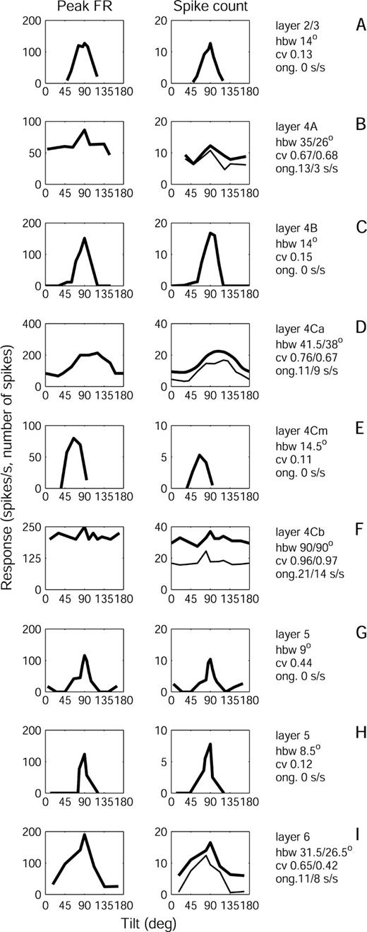
Orientation tuning curves based on spike counts and on peak firing rates for representative neurons in each of the cortical layers are displayed in Figure 2. These graphs show that very similar curves with a wide range of HBWs are derived by either measure. To obtain the estimates of peak firing rates, we calculated average response histograms with a 10 ms bin width, smoothed with a Gaussian with σ = 15 ms. Because the estimate of peak firing rate of cells with small receptive fields is easily degraded by averaging responses with small errors in correction for eye position, the midpoints of the individual responses were aligned to match the midpoint of the ensemble. This may produce a slight overcorrection for position errors, but it should be a more accurate way to estimate the peak rate. With this procedure, peak rates of most cells were high — between 75 and 250 spikes/s at the preferred orientation. However, because spike counts are less affected by position errors and are more amendable to correction for ongoing activity, they were used to derive the HBW and CV values reported in this paper.
Orientation tuning curves for representative neurons in V1 layers. All curves have been shifted on the horizontal axis so that the tuning curve is visualized as an uninterrupted peak. Left column: Tuning curves based on peak firing rate (FR). Right column: Tuning curves for the same cells based on mean spike count. Several responses to stimulus sweeps in the preferred direction were averaged. The text next to the tuning curves indicates the layer of origin, the half band width (hbw), the circular variance (cv) and the ongoing activity (ong) in spikes/sec (s/s) for each cell. For the four spontaneously active cells, in rows B, D, F and I, tuning curves derived from spike counts (right column) are shown before (thick line) and after (thin line) subtraction of ongoing activity measured during the stimulation trials. For these cells, text values before the slash (‘/’) show ongoing activity during viewing of a blank field, and hbw and cv derived without subtraction of ongoing activity, while values after the slash show ongoing activity during stimulation for orientation tuning, and hbw and cv derived after subtraction of ongoing activity.
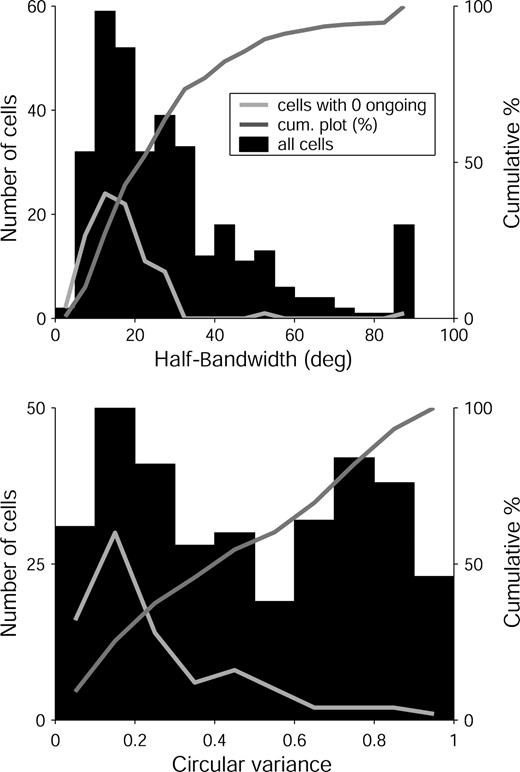
Neurons in V1 of alert monkeys show a wide range of selectivity for orientation (Fig. 3). The median HBW of the whole sample was 24° and the median CV was 0.45. However, both HBW and CV were unevenly distributed; most cells had low HBW and CV (see cumulative curve, Fig. 3) but there were also nonselective cells with HBW > 50° (49 cells, 14%) and CV > 0.6 (135 cells, 40%). The distribution of CV was significantly different from a unimodal distribution (Hartigan's dip test; P < 0.01), but the distribution of HBW did not differ statistically from unimodality. We compare these results with data from earlier studies in the Discussion.
Distributions of measures of orientation selectivity for our entire V1 sample (n = 339). Top panel: distribution of half-bandwidths measured at 1/(21/2) times the peak height (mean = 29°; median = 24°). Bottom panel: Distribution of circular variance (mean = 0.48; median = 0.45). Dark gray lines are the cumulative values (right vertical axes, in percent) for both measures. Light gray lines are the distributions for the subset of silent cells (n = 86) with 0 ongoing activity in the light.
Silent cells with no ongoing activity were particularly selective and they formed a large proportion of the narrowly tuned cells. Furthermore, we wish to emphasize that the narrowness of the tuning curves of the selective cells was not due to low responsivity. With near-optimal stimuli, neither the HBW (r = 0.13) nor the CV (r = 0.12) were significantly correlated with the peak firing rate. A previous analysis of orientation tuning in alert monkeys (Vogels and Orban, 1991) used flashed square-wave gratings of 8–10° in extent. With these large stimuli, the authors reported that cells with a larger orientation bandwidth had stronger responses (r = 0.4). This finding is consistent with an interpretation that the narrowly tuned cells have small fields with strong inhibitory inputs so that their responses would be reduced by the surround inhibition evoked by such a large stimulus (See Discussion).
Bandwidth and Circular Variance
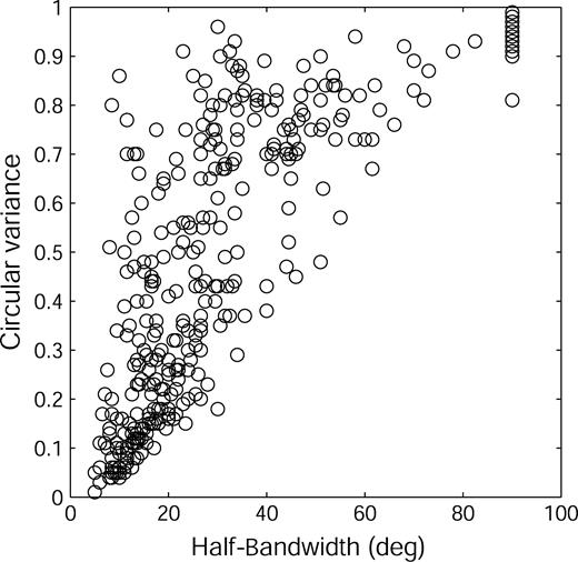
HBW and CV were highly correlated in alert animals (Fig. 4; r = 0.81; P < 0.01), as they are in anesthetized ones (Ringach et al., 2002b). This relationship was particularly evident for CV < 0.2 where all HBWs were < 20°. For larger CVs the correlation was not so tight; it was reduced by the contribution of cells with fairly narrow tuning around their preferred orientation, but an overall curve that did not go rapidly to zero. The HBW of these cells was relatively low while their CV was fairly large (cf. rows G and H of Fig. 2).
Scatterplot of circular variance versus half-bandwidth for the entire sample of 339 cells.
Orientation Selectivity and Receptive Field Size
There was a clear correlation between measures of receptive field width (Inc and Dec ARs and CRF) and orientation selectivity (Fig. 5); cells with small receptive fields were quite selective, while cells with large receptive fields were not. This is particularly evident for the HBWs of cells with small receptive fields; almost all cells with CRFs <20′ were very selective for orientation. Cells with CRFs ≤ 20′ (n = 72; Fig. 5, top row) had a median HBW of 14° and a median CV of 0.21, compared to a median HBW of 24° and a median CV of 0.45 for the whole sample. Cells with CRFs > 20′ showed more scatter in their HBW and CV than cells with smaller CRFs (Fig. 5, top row), but nevertheless the CRFs > 20′ were also positively correlated with HBW (r = 0.34; P < 0.001) and CV (r = 0.27; P < 0.001).
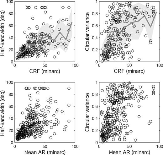
Relationship between orientation selectivity and receptive field dimensions. Left column: HBW versus CRF width (top panel, n = 242; r = 0.60, P < 0.01) and mean AR width (bottom panel, n = 339; r = 0.65, P < 0.01). Right column: CV versus CRF width (top panel, n = 242; r = 0.52, P < 0.01) and mean AR width (bottom panel, n = 339; r = 0.57, P < 0.01). Four points from cells with CRF widths > 100′ have been omitted to avoid excessive compression of the horizontal axis. Top row: Lines show mean HBW (left) and mean CV (right) calculated in 10′ bins. Shaded area denotes ± SD in each bin.
Orientation Selectivity and Ongoing Activity
If the level of ongoing activity is indicative of the amount of inhibition experienced by the cell (Snodderly and Gur, 1995) and if inhibition contributes to orientation selectivity, then it might be expected that ongoing activity should be related to orientation selectivity. Indeed, as illustrated in Figure 6, the breadth of orientation tuning and the ongoing activity were correlated (r = 0.67, P < 0.01 for HBW; r = 0.63, P < 0.01 for CV). The relationship between ongoing activity and orientation selectivity was particularly apparent for cells with very low ongoing activity (cf. Fig. 3). For the subset of cells with ongoing activity ≤1 spike/s (n = 122), the median HBW was only 15.2° and the median CV was 0.23.
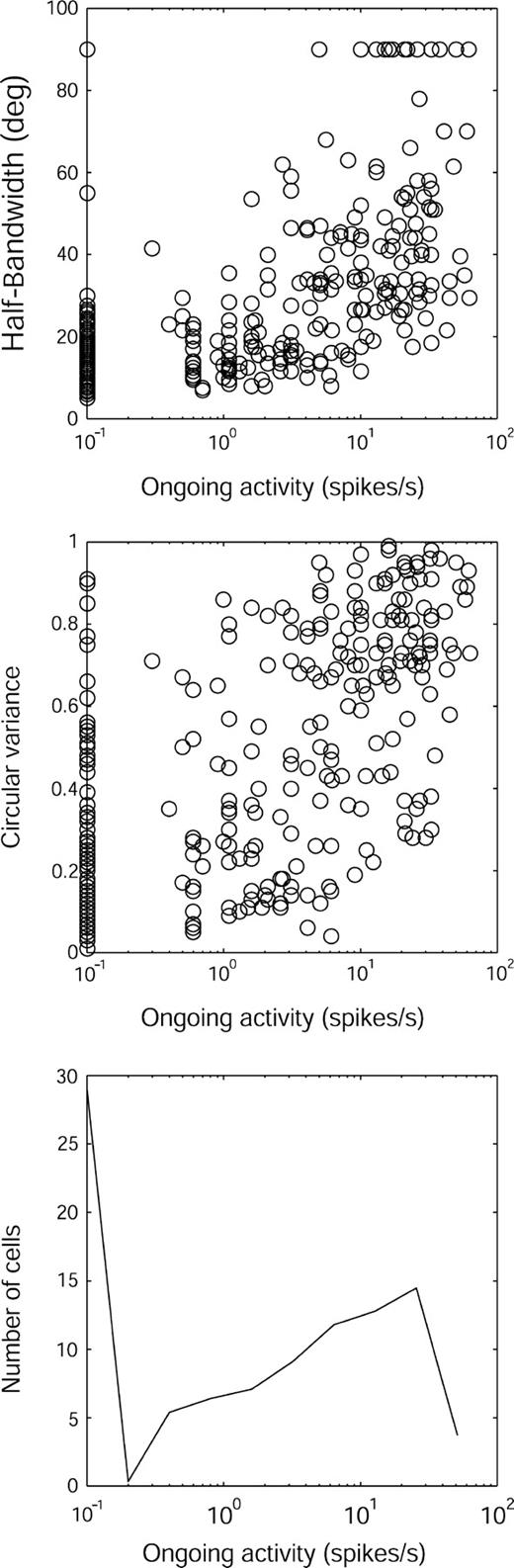
Distribution of orientation selectivity and its relationship to ongoing activity (spontaneous firing with a blank field of 1 or 5 cd/m2; n = 297). Top: Scatterplot of HBW versus ongoing activity. Middle: CV versus ongoing activity. Because the horizontal axis is a log scale, cells with zero ongoing activity are plotted at 0.1 spikes/s. Bottom: Distribution of ongoing activity in our total sample.
The distribution of ongoing activity was nonuniform (Fig. 6, bottom panel). Many cells (86/297) were completely silent, while a considerable number (71/297) were highly active (≥15 spikes/s). It is worth noting that 25/297 cells had ongoing activity ≥30 spikes/s.
Orientation Selectivity and Overlap Index
We have recently shown (Kagan et al., 2002) that the amount of overlap between receptive field ARs responding to increment and decrement bars is a robust criterion for distinguishing between simple and complex cells. In a subset of 218 cells for which the overlap index, OI, was measured, 35 cells were simple (OI ≤ 0.3) and 183 cells were complex (OI ≥ 0.5). OI was not correlated with either HBW (r = 0.14) or CV (r = 0.17, P > 0.01). Simple cells were slightly more tuned for orientation (median HBW, 17.0 ± 12.0°; CV, 0.36 ± 0.35) than complex cells (median HBW, 25.0 ± 32.5°, P < 0.01; CV, 0.50 ± 0.51, P < 0.05 by Mann–Whitney test), similar to results from anesthetized monkeys (Schiller et al., 1976b).
Orientation Selectivity and Relative Modulation
For cells studied with drifting gratings, the degree of relative modulation (RM) calculated for maximum response or maximum modulation (see Materials and Methods) was not correlated with either HBW or CV (all |r| < 0.1).
Orientation Selectivity and Surround Suppression
To study the relation between surround suppression and orientation selectivity we measured responses of 67 cells to optimally oriented stationary, flashing bars of increasing widths. The bars were centered on the receptive field while dynamically correcting for changes in eye position as described in Materials and Methods. The reduction of maximal response caused by a bar twice the CRF width as a function of HBW and CV, is shown in Figure 7. Both HBW (r = − 0.62; P < 0.01) and CV (r = − 0.59; P < 0.01) were clearly correlated with the effectiveness of suppression. Even at this modest bar width, almost all cells were suppressed to some extent but those more selective for orientation were more strongly suppressed than the less-selective cells. Cells with HBW < 20° and CV < 0.3 reduced their responses by larger amounts (mean 67.5% and 65%, respectively) than cells with HBW > 30° and CV > 0.50 (mean 32% and 36.3%, respectively).
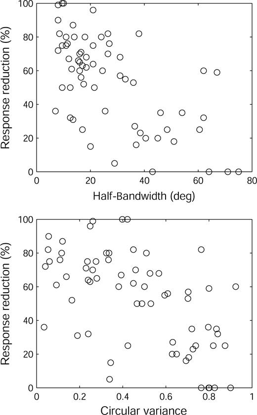
Scatterplots of HBW (top) and CV (bottom) versus response reduction (% of response to an optimal bar). The stimulus was a flashing, optimally oriented bar twice as wide as the CRF.
Relationship of Direction Selectivity to Orientation Selectivity
There was a bimodal distribution of our current sample into 73 (23%) directional cells (DI ≥ 0.5) and 250 (77%) nondirectional (DI < 0.5) ones (Fig. 8). For the whole sample, there was a weak but significant correlation between DI and HBW (r = −0.34, P < 0.01) and DI and CV (r = −0.32, P < 0.01). The scatterplots in Fig. 8 show how the directional and nondirectional groups differ; the nondirectional cells include a much higher proportion of neurons with broad orientation tuning. Consequently, as a group, directional cells (HBW: median, 14.5°, ± interquartile range 13.38; CV, 0.21 ± 0.29) are more orientation selective (P < 0.01, Mann–Whitney test) than nondirectional ones (median HBW, 26.5° ± 25.5; CV, 0.55 ± 0.51).
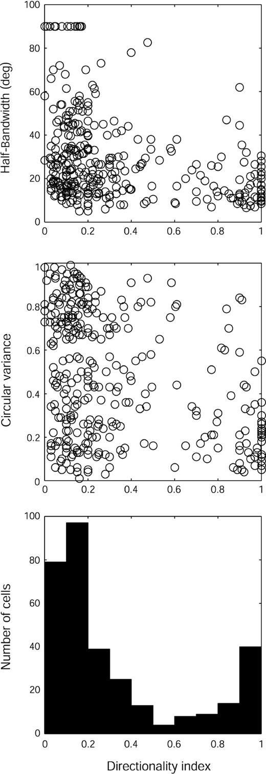
Distribution of direction selectivity and its relationship to orientation selectivity. Directionality index (DI) values (n = 323) are averages of DI measured with increment and decrement bars. Top: Scatterplot of HBW versus directionality index (cells with DI ≥ 0.5 are considered direction-selective). Middle: CV versus directionality index. Bottom: Distribution of DI values in our total sample.
Direction Selectivity and Ongoing Activity
Another feature that direction-selective cells share with other tightly oriented cells is low ongoing activity. Cells with DI ≥ 0.5 had median ongoing activity of only 0.1 ± 2.6 spikes/s (n = 64), whereas the values for the nondirectional group (DI < 0.5) were 4.1 ± 15.5 spikes/s (n = 225), a highly significant difference (P < 0.0001, Mann–Whitney test). This difference occurred in spite of the fact that ∼25% of nondirectional cells had 0 ongoing rate. The correlation between ongoing activity and DI was −0.35 (P < 0.01, n = 289).
Direction Selectivity and Receptive Field Characteristics
Because orientation tuning is narrower for cells with smaller CRFs and smaller ARs, and direction selectivity is correlated with orientation selectivity, it follows that direction-selective cells should have relatively small CRFs and ARs. Indeed, the direction-selective cells (n = 76) had mean ARs that were smaller (15 ± 17′) than those of the nondirectional group (26.2 ± 21.9′, n = 252; P < 0.0001, Mann–Whitney test). The correlation between DI and mean AR was small, but significant (r = −0.31, P < 0.01). Similarly, just as simple cells were slightly more selective for orientation than complex cells, they were also slightly more biased for direction of movement (median DI 0.3 versus 0.17; P < 0.01 by Mann–Whitney test).
Conjunctions of Physiological Properties of V1 Cells
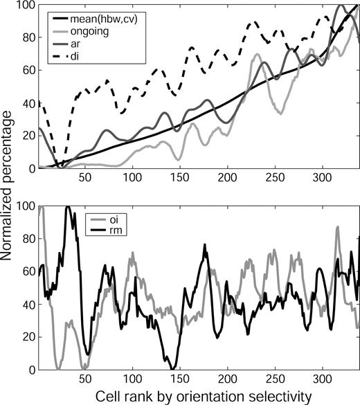
To illustrate how six of the physiological features discussed above covary, a combined measure of orientation selectivity was created by taking the mean of the normalized values of the CV and HBW, and sorting all cells in our sample according to this mean. The results of this procedure are displayed in Figure 9. The upper panel shows that orientation selectivity, ongoing activity, AR width and direction selectivity covary. For example, if a cell is silent, it is also likely to be selective for both orientation and direction and have small ARs. The direction selectivity curve is more ragged than the other curves, reflecting our findings (above) that while strongly directional cells are usually silent, tightly oriented and have small ARs, less pronounced direction biases are only weakly correlated with other features.
Conjunctions of physiological properties of V1 cells. Cells were ranked according to the mean of their CV and HBW values as an indicator of their orientation selectivity. Data for each parameter were normalized to a value of 100, smoothed by a 31 point sliding Hanning window, and then renormalized. Top: Relationship between orientation selectivity and ongoing activity, mean AR width and the inverse of the direction index, DI. Bottom: Lack of relationship between orientation selectivity and ovelap index, OI, or relative modulation, RM.
In contrast to the covariation of features displayed in the upper panel of Figure 8, the lower panel shows that overlap index and relative modulation do not covary with the other features.
Laminar Distributions of Neuronal Characteristics
Orientation Selectivity
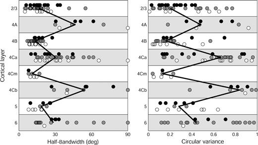
Here we show that orientation selectivity is nonuniformly distributed across the cortical layers, with a higher proportion of nonselective cells in the input layers 4A, 4C and 6. In Figure 10 values for HBW and CV are plotted for cells that could be assigned to a laminar location. The procedure for assignments using three levels of confidence is described in the Materials and Methods. Since the pattern of alternation of those measures for each of the three levels of confidence was very similar, all data were combined to compute median values for each layer. For both HBW and CV there is a clear alternation of orientation selectivity with the layer of origin. Almost all cells in layer 4Cβ were nonoriented, which is consistent with most earlier findings (Poggio et al., 1977; Bauer et al., 1980; Bullier and Henry, 1980; Dow et al., 1981; Blasdel and Fitzpatrick, 1984; Hawken and Parker, 1984; Livingstone and Hubel, 1984; Leventhal et al., 1995; Snodderly and Gur, 1995; but see Ringach et al., 2002b, for a contrary finding). Note that HBWs of cells in layers with low selectivity are widely distributed while the distribution is much tighter in the selective layers.
Laminar pattern of orientation selectivity in V1 of alert monkeys. Left panel: HBW. Right panel: CV. Each point represents a cell (n = 170) and different symbols represent different levels of confidence (see Materials and Methods) in the assignment. Filled circles = level 1; gray circles = level 2; open circles = level 3. Vertical offsets have been added to separate the symbols. The zigzag vertical line connects the median values for cells in different layers.
In many penetrations we noticed a lull in spontaneous activity along a stretch of less than 100 μm between what we concluded were layers 4Cα and 4Cβ. This quiet region with no background activity was in stark contrast to the lush spontaneous background of 4Cα and the buzzing background of 4Cβ. This drop in spontaneous activity has previously been noticed by DeYoe et al. (1995, their Fig. 7). We have data from 12 single cells from this area and their characteristics are so different from either 4Cα or 4Cβ cells that it bolsters our confidence that this region is a distinct layer. All seven cells for which we had orientation tuning curves were highly oriented (HBW: 7–19, median = 11.5°; CV: 0.04–0.23, median = 0.13); most cells (9/12) were directional (DI ≥ 0.9); 11/12 had no maintained discharge or a very low one (0–2 spikes/s; median = 0 spikes/s), and 11/12 had small CRFs (5–24′; median = 12′). One exceptional cell with a receptive field at an eccentricity near the extreme of our sample (∼10°) had a relatively large CRF and moderate ongoing activity.
Anatomical evidence from several laboratories (Yoshioka et al., 1994; Yabuta and Callaway, 1998; Boyd et al., 2000; Sawatari and Callaway, 2000; Lund et al., 2003) suggests a distinct anatomical and physiological role for the middle of layer 4C as the first location where magno- and parvocellular interaction takes place. Following their lead, we call this silent, narrow layer between 4Cα and 4Cβ, mid 4C (4Cm). We would like to emphasize that physiological localization of 4Cm requires sequence information during the recordings, which we obtained by using the bands of spontaneous activity that occur immediately above and below 4Cm. Traditional marking techniques, such as electrolytic lesions, do not have the resolution to distinguish such a narrow region.
Ongoing Activity and AR Width
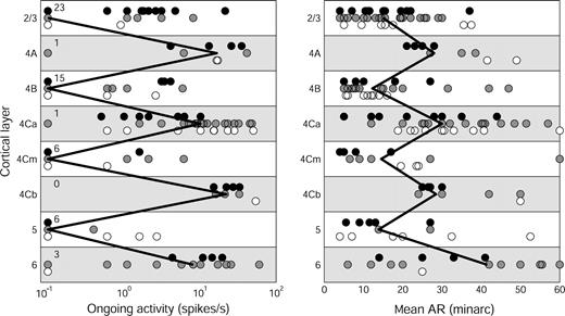
Since present data show that orientation selectivity is correlated with ongoing activity and receptive field width, we examined how the laminar distributions of these characteristics compare with the distribution of orientation selectivity (Fig. 11). Because we did not have measurements of both Inc and Dec ARs for all the cells that could be assigned to layers, we have used the mean AR width as our indicator of receptive field width. When both Inc and Dec data were available, the mean of the two was used, but when data were available for only one AR, or the cell responded only to one sign of contrast, a single AR width was used as the value for the cell. A control analysis of 242 cells for which both Inc and Dec data were collected showed that the mean AR width was highly correlated with the CRF width (r = 0.95), so it is an appropriate surrogate for the CRF width for determining the laminar pattern. Cells with small ARs and low ongoing activity were found in layers 2/3, 4B, 4Cm, and 5 and those with larger ARs and higher ongoing activity in layers 4A, 4Cα, 4Cβ and 6. This distribution pattern is similar to the one we presented previously (Snodderly and Gur, 1995), with the addition of the newly recognized sublamina 4Cm. There is a striking similarity between the alternating pattern for AR size, ongoing activity, and orientation selectivity.
Laminar distribution of ongoing activity and AR width in V1 of alert monkeys. Left panel: Ongoing activity during presentation of a blank field (n = 160). Note logarithmic scale. Cells with zero ongoing activity are plotted as 0.1 spikes/s, and the number of cells with zero ongoing activity is indicated to the right of the vertical axis because many data points are overlapping. Right panel: Mean AR width of cells assigned to cortical layers (n = 175). Three cells in layer 6 with mean AR > 60′ are plotted as 60′ to avoid compressing the x-axis. Other conventions as in Figure 10.
Direction Selectivity
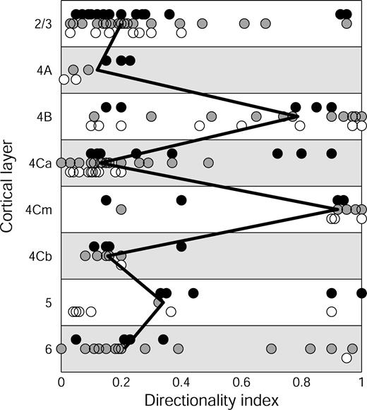
Previous reports have emphasized that direction-selective cells are mainly found in layers 4B, 4Cα and 6, which receive either direct or second-stage inputs dominated by the magnocellular pathway (Snodderly and Gur, 1995, and references therein). However, the laminar distribution shown in Figure 12 differs from earlier results in having strongly direction-selective cells in several other cortical layers as well. Two factors account for our new results. First, the recognition of 4Cm as a separate layer with cells that are direction-selective as well as being narrowly tuned for orientation. Second, the clear localization of direction-selective cells to layers 2/3 and 5. For the 6 cells with DI ≥ 0.9 in these two layers, at least four had no ongoing activity, and the largest AR width was 15′. It is worth noting that in layers 2/3 and 5, 7 of eight direction-selective cells for which we had analog spike data had large spikes (1.4–4 mV) with a dominant negative lobe, and recordings were stable for a long time. It is thus likely that these direction-selective cells are large pyramidal cells (Gur et al., 1999). We believe the belated recognition of this group of direction-selective cells is due to sampling bias, as elaborated in the Discussion. Given the small number of cells assigned to layers 5 and 6, the relative proportions of direction-selective cells indicated for those layers may be unrepresentative and they should be investigated in more detail with a larger sample.
Laminar distribution of direction selectivity in V1 of alert monkeys. The direction index, DI, was measured for 169 of the cells that could be assigned to layers. Conventions same as Figure 10.
Discussion
Many previous studies (see Introduction) have shown that V1 has a highly differentiated organization of orientation selectivity and spontaneous activity. Layers with low spontaneous activity typically contain cells more sharply tuned for orientation. In contrast, a nearly uniform distribution of these physiological properties in V1 has been reported by Ringach et al. (2002b), who found a broad distribution of orientation selectivity in all cortical layers. These results raise important questions about the relationship of orientation selectivity to other physiological properties and to the anatomical organization of V1.
As part of our studies of V1 of alert monkeys we have examined the relation between orientation selectivity (HBW and CV) and several physiological characteristics. Our work shows, for the first time, that cells highly selective for orientation have a suite of distinctive properties; they tend to have low ongoing activity, small CRFs, and they dominate the direction-selective cells. The receptive field organization of the selective cells includes strong surround suppression (Fig. 7) that is probably a major contributor to these properties (see also Ringach et al., 2002a). On the other hand, orientation selectivity is not correlated with overlap index or relative modulation, indicating that the latter features are generated by different mechanisms.
This report is the first quantitative description of the laminar and sublaminar distribution of orientation selectivity in V1 of alert monkeys. We have compared the laminar distribution of orientation selectivity with the distribution of CRF widths, ongoing activity and direction selectivity to present a more integrated view of V1 organization than is obvious from previous studies. Our quantitative results are consistent with earlier, qualitative, findings and differ from the findings of Ringach et al. (2002b). We find that layers that receive direct LGN input (4A, 4Cα, 4Cβ and 6) have cells that are less tuned for orientation than layers that do not receive direct LGN input (2/3, 4B, 4Cm and 5). Similar alternating patterns of laminar properties are seen for orientation selectivity, ongoing activity and CRF width, with a more complex distribution of direction selectivity. As part of this description, we present the first physiological evidence to support the anatomical delineation of a distinct sublamina, 4Cm, located between 4Cα and 4Cβ. The properties of 4Cm cells show that selectivity emerges almost immediately in striate cortex without requiring many synaptic relays.
We have shown (Gur et al., 1999) that conjunctions of physiological characteristics may be found not only across but also within laminae. Small- and large-spike cells recorded with the same electrode clearly differ; the small cells are more spontaneous, have larger CRFs and are less selective for orientation than the large cells. The association of these characteristics probably indicates the importance of intracortical inhibition in generating stimulus selectivity and CRF size. Strong inhibitory inputs may account for lack of spontaneous activity, narrow ARs and strong orientation selectivity. For a cell also to be direction selective, the inhibitory mechanisms must have an intricate spatiotemporal arrangement.
Our finding that cells selective for orientation are strongly suppressed by a stimulus extending beyond the CRF may be another indication of the importance of inhibition in shaping properties of V1 neurons (Freeman et al., 2002). Cells not suppressed by a large stimulus were not selective for orientation, had large CRFs and were spontaneously active. These are probably the same kind of cells described by Kinoshita and Komatsu (2001) as luminance or brightness cells. We suggest that different amounts of inhibition result in cells with radically different specializations. The strongly inhibited cells are selective for fine, localized spatial information, while weakly inhibited cells respond to more global properties such as surface brightness.
There is a lively debate about the mechanisms responsible for the dramatic emergence of orientation selectivity in V1 (see reviews by Ferster and Miller, 2000; Shapley et al., 2003). The different levels of orientation selectivity in different laminae indicate that there is no single mechanism generating orientation selectivity (Schwark et al., 1986) but that in different laminae there are different balances between excitatory and inhibitory mechanisms. It is reasonable to suggest, for example, that the broad orientation tuning in 4Cα is generated mostly by a feed-forward mechanism with some modest intra-cortical inhibition, while the very strong orientation selectivity found in the output layers reflects additional inhibitory mechanisms (e.g. Alonso et al., 2001; Martinez et al., 2002; Shapley et al., 2003). While the median values of orientation selectivity clearly differ in input versus output layers, there is also much larger variation in the selectivity of individual cells in the input layers. This may indicate that transformation to more selective responses begins immediately within the input layers (Gur et al., 1999).
Comparisons with Earlier Studies
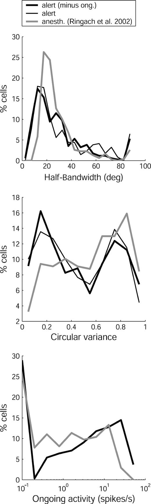
Certain aspects of V1 organization appear to be clearer in alert than in anesthetized monkeys. Data from alert and from anesthetized monkeys are compared for three pertinent features in Figure 13. The bottom panel shows that the largest single group of cells recorded from both preparations showed no ongoing activity, but alert monkeys had a clear second lobe in the distribution that included many cells firing tens of spikes per second. This high activity probably reflects the tonic input from the lateral geniculate nucleus (LGN), where many cells fire at rates >24 spikes/s (D.M. Snodderly, DM. Snodderly and M. Gur, unpublished results; Y. Kayama, personal communication). In contrast, spontaneous activity of LGN cells of anesthetized monkeys is said to be low (Shapley et al. 2003). If the strong tonic activity in the alert LGN drives both excitatory and inhibitory processes, the resulting cortical properties could be more finely balanced and more differentiated. We suggest that subtle differences in this balance contribute to more uneven distributions of individual features in alert monkeys and to the striking alternation of ongoing activity and other features associated with the cortical laminae.
Comparison of results from alert (our study) and anesthetized (Ringach et al., 2002b) monkeys. Top panel: Black lines. Half-bandwidth of V1 neurons in alert monkeys (n = 339), with subtraction (thick line) and without subtraction (thin line) of ongoing activity (ong.). Gray line. Half-bandwidth of V1 neurons in anesthetized monkeys (n = 308) without subtraction of ongoing activity. Data from alert monkeys were collected with drifting bars as described in the Materials and Methods, and control experiments were conducted with drifting gratings, as described in the Results. Data from anesthetized monkeys were collected with drifting gratings. Middle panel: Circular variance for the same sets of neurons. Bottom panel: Distributions of ongoing activity of V1 neurons in alert (n = 297) and anesthetized (n = 308) monkeys. Data were collected during viewing of a blank, uniform field of 1 cd/m2 for alert monkeys and 55–65 cd/m2 for anesthetized ones. Cells with no ongoing activity were assigned a value of 0.1 to accommodate the log scale. Values in all panels are plotted as percentages of the total sample for ease of comparison. Note that for alert monkeys, the distributions of HBW and CV are similar whether or not ongoing activity is subtracted from the responses (r = 0.92, r = 0.88, respectively, P < 0.01).
A similar distinction is seen in the distribution of circular variance (Fig. 13, middle panel). While the data from anesthetized monkeys showed no clear pattern, the distribution from alert monkeys was bimodal and the dip in the distribution is statistically significant. Although oriented and non-oriented cells have been distinguished qualitatively in the past (e.g. Livingstone and Hubel, 1984; Snodderly and Gur, 1995), this is the first quantitative differentiation of cell groups with high and low orientation selectivity. The differentiation achieved by the CV measure probably reflects its ability to distinguish cells that have different degrees of off-peak inhibition, which is not accomplished as well by the HBW measure (Fig. 13, top panel; see also Fig. 3). However, since most previous studies of orientation selectivity used only HBW as a measure, we refer to it for comparison with earlier work.
Our sample includes many cells with narrow bandwidths (26% have HBW < 15°) and similar percentages of sharply tuned cells have been reported by others for both anesthetized (Schiller et al. 1976b; DeValois et al., 1982) and alert (Vogels and Orban, 1991) monkeys. In contrast, the sample of Ringach et al. includes fewer highly selective cells, with only 6% having HBW < 15°. Whether this difference arises from the particular anesthetic regimen used or other factors remains to be seen.
In general, our data from alert monkeys show stronger relationships among physiological parameters than previously reported for anesthetized animals. For example, direction-selective cells had smaller HBWs (median 14.5°) than nondirectional cells (median 25.5°). This difference was not apparent in initial data from anesthetized monkeys (Schiller et al., 1976b), and the correlation (r = −0.34) between HBW and DI in our data was stronger than the value reported for anesthetized monkeys (r = −0.17; DeValois et al., 1982).
There was also a strong relationship in alert animals between HBW and ongoing activity (r = 0.67). For data from anesthetized animals, where ongoing activity is diminished (Snodderly and Gur, 1995), a weaker correlation between HBW and ongoing activity has been reported (Ringach et al., 2002b; r = 0.51, personal communication). The strong relationship we found is linked to the fact that broadly tuned cells were preferentially located in layers with high ongoing activity. The distinctive pattern of alternating layers of high and low ongoing activity in V1 of alert animals thus provides important clues to the functional organization and the distribution of stimulus selectivity in the cortex. Furthermore, it is closely related to the functional anatomy, because the distribution of ongoing activity corresponds to the pattern of cytochrome oxidase staining in V1 (Livingstone and Hubel, 1984; DeYoe et al., 1995; Snodderly and Gur, 1995). This correspondence has an appealing interpretation, because it implies that spontaneous activity and relatively unselective stimulus-driven activity, that together consume large amounts of energy, occur preferentially in regions where lots of energy is generated. The extremely selective cells, on the other hand, are less active overall, less energy is needed to support them, and they can function efficiently in regions with a lower metabolic rate.
4Cα/4Cβ–4Cm–3B — a high resolution pathway?
We have presented the first physiological evidence of a functionally distinct layer, 4Cm, located between 4Cα and 4Cβ (Yoshioka et al., 1994). Responses of cells in this sublayer differ dramatically from those in either 4Cα or 4Cβ; they have very low ongoing activity, small CRFs, are highly oriented and most are very directional. 4Cm receives input from both 4Cα and 4Cβ — input that is highly spontaneous and only moderately selective for spatial features. The very selective properties of 4Cm cells must thus be generated by strong inhibitory mechanisms, consistent with the suggestion of Lund et al. (2003).
Anatomical evidence (reviewed by Boyd et al., 2000) shows that 4Cm axons project to layer 3B, but in spite of the presence of these inputs that we now recognize as direction selective, direction selectivity has not usually been reported in layer 2/3. Indeed, in our earlier study of laminar organization of V1 (Snodderly and Gur, 1995), we found only one direction-selective cell in this layer. Thus, the laminar distribution of direction selectivity we report now differs both from our earlier results (Snodderly and Gur, 1995), and from data collected from anesthetized animals in several laboratories (Livingstone and Hubel, 1984; Orban et al., 1986; Hawken et al., 1988). Those reports emphasized layers 4B, 4Cα and 6 as the main locations for direction-selective cells, prompting Lund (1990) to ask why direction selectivity is not commonly found in the superficial layers of the cortex, given that the superficial layers receive strong inputs from layer 4B. This apparent contradiction is even more stark with the realization that there is also direction-selective input to the superficial layers from 4Cm.
We are now reporting that direction-selective cells are more broadly distributed in the cortex, including layers 2/3. We believe the belated recognition of this fact is because of the smaller ARs and the extreme stimulus selectivity of many of the direction-selective cells. Particularly in layer 2/3, cells are often narrowly tuned for orientation as well as being end-inhibited or side-inhibited, or both, giving rise to their characterization as ‘persnickety’ (Judge et al, 1980b). In many penetrations, at a depth consistent with layer 3B, we have recorded from large-spike cells, presumably large pyramidal cells (Gur et al., 1999) that were very hard to stimulate. In fact, if it were not for the cells being stimulated when the monkey was looking around between trials, we would not have been aware of their existence. We noted that these cells typically fired short bursts at very high instantaneous rates (>500 spikes/s).
With additional experience, we have been able to characterize some of these more demanding cells. The new results, and their relationship to the known anatomy, justify postulating the existence of a high-resolution path in V1. This path originates in the convergence of inputs from the magno- and parvocellular input layers (Nealey and Maunsell, 1994; Yoshioka et al., 1994) onto 4Cm cells generating silent, directional cells with small CRFs. These cells synapse on layer 3B cells where additional, perhaps intralaminar processing (Gur et al., 1999; Chisum et al., 2003) creates cells that are extremely selective for stimulus properties — on a par with our best perceptual abilities. Since these cells are completely silent most of the time, their activity, which usually consists of just a few spikes per response, could be of great importance for perception.
The concept of V1 that emerges from our studies is a precisely organized area composed of diverse components. The differences among the specialized components are easier to recognize in alert monkeys than in anesthetized animals because the physiological relationships are stronger and distinctions among the cortical laminae are clearer. As we have argued previously (Snodderly and Gur, 1995), the correspondence between physiology and anatomy is more apparent in the waking brain. The alternating laminar pattern of stimulus selectivity and ongoing activity may offer important clues to the principles underlying construction of the complex network of the primary visual cortex.
We thank Andrzej Przybyszewski for participating in some of the experiments and Beth Scherer for technical assistance. Dario Ringach, Mike Hawken, and Robert Shapley gave useful comments on the manuscript. Supported by NIH EY12243.
References
Alonso JM, Usrey WM, Reid RC (
Bauer R, Dow BM, Vautin RG (
Blasdel GG, Fitzpatrick D (
Boyd JD, Mavity-Hudson JA, Casagrande VA (
Bullier J, Henry GH (
Chisum HJ, Mooser F, Fitzpatrick D (
DeValois RL, Yund EW, Hepler N (
DeYoe EA, Trusk TC, Wong-Riley MTT (
Dow BM, Snyder AZ, Vautin RG, Bauer R (
Eckhorn R, Thomas U (
Everson RM, Prashanth AK, Gabbay M, Knight BW, Sirovich L, Kaplan E (
Ferster D, Miller KD (
Foster KH, Gaska JP, Nagler M, Pollen DA (
Freeman TCB, Durand S, Kiper DC, Carandini M (
Gur M, Snodderly DM (
Gur M, Snodderly DM (
Gur M, Snodderly DM (
Gur M, Beylin A, Snodderly DM (
Gur M, Beylin A, Snodderly DM (
Hawken MJ, Parker AJ (
Hawken MJ, Parker AJ, Lund JS (
Hubel DH, Wiesel TN (
Hubel DH, Wiesel TN (
Judge SJ, Richmond BJ, Chu FC (
Judge SJ, Wurtz RH, Richmond BJ (
Kagan I, Gur M, Snodderly DM (
Kinoshita M, Komatsu H (
Leventhal AG, Thompson KG, Liu D, Zhou Y, Ault SJ (
Livingstone MS, Hubel DH (
Lund JS (
Lund JS, Angelucci A, Bressloff PC (
Martinez LM, Alonso JM, Reid RC, Hirsch JA (
Nealey TA, Maunsell JH (
Orban GA (
Orban GA, Kennedy H, Bullier J (
Pettigrew JD, Nikara T, Bishop PO (
Poggio GF, Doty RW, Jr, Talbot WH (
Ringach DL, Bredfeldt CE, Shapley RM, Hawken MJ (
Ringach DL, Shapley RM, Hawken MJ (
Robinson DA (
Sawatari A, Callaway EM (
Schiller PH, Finlay BL, Volman SF (
Schiller PH, Finlay BL, Volman SF (
Schwark HD, Malpeli JG, Weyand TG (
Shapley R, Hawken M, Ringach DL (
Skottun BC, De Valois RL, Grosof DH, Movshon JA, Albrecht DG, Bonds AB (
Snodderly DM (
Snodderly DM, Gur M (
Snodderly DM, Kagan I, Gur M (
Vogels R, Orban GA (
Yabuta NH, Callaway EM (
Author notes
1Department of Biomedical Engineering, Technion, Israel Institute of Technology, Haifa 32000, Israel, 2Schepens Eye Research Institute, Boston, MA 02114, 3Department of Ophthalmology, Harvard Medical School, Boston, MA 02115, USA and 4Program in Neuroscience, Harvard Medical School, Boston, MA 02115, USA