


Abstract
Extraclassical receptive field phenomena in V1 are commonly attributed to long-range lateral connections and/or extrastriate feedback. We address 2 such phenomena: surround suppression and receptive field expansion at low contrast. We present rigorous computational support for the hypothesis that the phenomena largely result from local short-range (<0.5 mm) cortical connections and lateral geniculate nucleus input. The neural mechanisms of surround suppression in our simulations operate via (A) enhancement of inhibition, (B) reduction of excitation, or (C) action of both simultaneously. Mechanisms (B) and (C) are substantially more prevalent than (A). We observe, on average, a growth in the spatial summation extent of excitatory and inhibitory synaptic inputs for low-contrast stimuli. However, we find this is neither sufficient nor necessary to explain receptive field expansion at low contrast, which usually involves additional changes in the relative gain of these inputs.
Introduction
In mammals, the very first stage of cortical visual processing takes place in the striate cortex (area V1). Already at this level, spatial summation of visual input is considerably complex. This is manifest from the fact that cells in V1 display a set of phenomena that are conventionally referred to as “extraclassical receptive field phenomena.” In this paper, we focus on 2 such phenomena, surround suppression (suppression for increasing stimulus size, “size tuning”) and the increase of the receptive field size at low contrast. These 2 phenomena are observed throughout the striate cortex, including all cell types in all layers and at all eccentricities (Schiller and others 1976; Dow and others 1981; Silito and others 1995; Kapadia and others 1999; Sceniak and others 1999, 2001; Anderson and others 2001; Cavanaugh and others 2002; Ozeki and others 2004). The suppression seen is substantial, with cells in macaque V1 showing, on average, a 30–40% reduction in their firing rates at large stimulus sizes (Cavanaugh and others 2002). Similarly significant is the receptive field expansion at low contrast. Typical is a doubling in receptive field size when stimulus contrast is reduced by a factor of 2–3 (Sceniak and others 1999). Apparently, at low contrast, neurons in V1 sacrifice spatial sensitivity in return for a gain in contrast sensitivity (Sceniak and others 1999). Neural mechanisms responsible for these 2 phenomena are at present poorly understood. Understanding these mechanisms is potentially important for developing a theoretical model of early signal integration and neural encoding of visual features in V1.
Popular working hypotheses are that these 2 extraclassical receptive field phenomena are a product of long-range horizontal connections (DeAngelis and others 1994; Dragoi and Sur 2000; Hupé and others 2001; Stettler and others 2002) and/or feedback from extrastriate areas (Sceniak and others 2001; Angelucci and others 2002; Cavanaugh and others 2002; Bair and others 2003). Arguments in support of these hypotheses are based on the observed surround sizes and the cortical magnification factor and claim that short-range (<0.5 mm) and even long-range horizontal (<5 mm) connections in V1 would not have sufficient spatial extent to be responsible for surround suppression or receptive field expansion (Sceniak and others 2001; Cavanaugh and others 2002). Further, support along this line was presented using anterograde and retrograde tracer injections (Angelucci and others 2002) and timing experiments (Bair and others 2003). So far, however, these hypotheses are based on indirect experimental observations and also lack rigorous computational support.
The hypothesis that the phenomena result from local short-range (<0.5 mm) cortical connections and lateral geniculate nucleus (LGN) input is largely ignored or dismissed. However, support for it can be found in the experimental data. For instance, surround suppression and receptive field expansion at low contrast are significant throughout V1 (Sceniak and others 1999, 2001), including in layers that do not receive extrastriate feedback and do not have long-range horizontal connections. Both phenomena have been observed in the LGN and are likely to be partially inherited by V1 via the feed-forward input from the LGN (Solomon and others 2002; Ozeki and others 2004). Finally, there is experimental evidence for contextual modulations mediated by local short-range connections in cats (Das and Gilbert 1999).
In this paper, we suggest neural mechanisms for surround suppression and receptive field expansion in layers 4Cα and 4Cβ of macaque V1. We show that local short-range cortical connections and LGN input are, in principle, sufficient to explain a major part of the phenomena. We do this by means of a large-scale neural network model that is constructed, as much as possible, from established experimental data. We suggest neural mechanisms for the phenomena by analyzing the synaptic inputs that generate them in the model. An illustration of the model's architecture is given in Figure 1. A brief summary of the model is given in Methods.
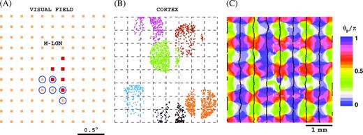
Model architecture. (A) A select cluster of ON (blue circles) and OFF (red dots) magno-LGN cells that feed into 1 cortical cell. Receptive field centers of LGN cells are organized on a square lattice (orange). (B) Select M-LGN axons in our model-V1. Points of the same color are cortical cells that connect to the same LGN cell. (C) Pinwheel structure and ocular dominance columns for M10 model, constructed from averaged responses in the spirit of optical imaging experiments (Blasdel 1992). Samples used to analyze the 2 extraclassical phenomena are made up of cells from within the white dashed rectangle (see Methods for details).
Methods
The Model
Our model consists of 8 ocular dominance columns and 64 orientation hypercolumns (i.e., pinwheels), representing a 16-mm2 area of a macaque V1 input layer 4Cα or 4Cβ. The model contains approximately 65 000 cortical cells and the corresponding appropriate number of LGN cells. Our cortical cells are modeled as conductance-based integrate-and-fire point neurons, 75% are excitatory cells and 25% are inhibitory cells. Our LGN cells are half-wave rectified spatiotemporal linear filters. The model is constructed with isotropic short-range cortical connections (<500 μm), realistic LGN receptive field sizes and densities, realistic sizes of LGN axons in V1, and cortical magnification factors and receptive field scatter that are in agreement with experimental observations. We will only give a very brief description of the model here; it is explained in detail in Supplementary Materials. Some background information can also be found in previous works (McLaughlin and others 2000; Wielaard and others 2001) by one of the authors (J.W.).
 for
for  The terms are the contributions from the cortical excitatory (μ = E) and inhibitory (μ = I) neurons and include only isotropic connections,
Summary of basic notation used in the paper
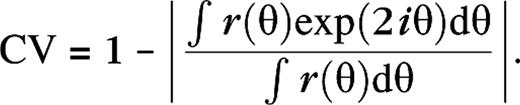
| CV | Circular variance (eq. 11) |
| F0s, F1s, F2s | Mean, first, and second harmonic of the cycle-trial–averaged spike train |
| F0v, F1v, F2v | Mean, first, and second harmonic of the cycle-trial–averaged membrane potential |
| gE, gI, gLGN | Excitatory and inhibitory conductance and conductance of the LGN input of V1 cells |
| M0, M10 | Magnocellular versions of the model at 0° and 10° eccentricity |
| P0, P10 | Parvocellular versions of the model at 0° and 10° eccentricity |
| rA | Aperture radius (size of the stimulus) |
| r+, r− | Receptive field sizes (radius) for high (+) and low (−) contrast stimuli. In some cases it is indicated for which response measure they are evaluated (e.g., spike responses, r+(s)) |
| R+, R− | Surround sizes (radius) for high (+) and low (−) contrast stimuli |
| 〈S(t)〉 | Firing rate (cycle-trial–averaged spike train) in spikes per second |
| 〈v(t)〉 | Cycle-trial–averaged membrane potential |
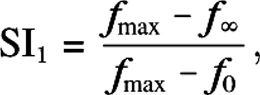
| SI1 | Suppression index (eq. 7) similar to that used in Cavanaugh and others (2002) |
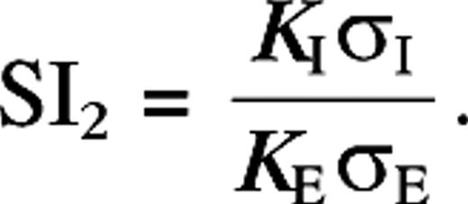
| SI2 | Suppression index (eq. 9) similar to that used in Sceniak and others (2001) |
| CV | Circular variance (eq. 11) |
| F0s, F1s, F2s | Mean, first, and second harmonic of the cycle-trial–averaged spike train |
| F0v, F1v, F2v | Mean, first, and second harmonic of the cycle-trial–averaged membrane potential |
| gE, gI, gLGN | Excitatory and inhibitory conductance and conductance of the LGN input of V1 cells |
| M0, M10 | Magnocellular versions of the model at 0° and 10° eccentricity |
| P0, P10 | Parvocellular versions of the model at 0° and 10° eccentricity |
| rA | Aperture radius (size of the stimulus) |
| r+, r− | Receptive field sizes (radius) for high (+) and low (−) contrast stimuli. In some cases it is indicated for which response measure they are evaluated (e.g., spike responses, r+(s)) |
| R+, R− | Surround sizes (radius) for high (+) and low (−) contrast stimuli |
| 〈S(t)〉 | Firing rate (cycle-trial–averaged spike train) in spikes per second |
| 〈v(t)〉 | Cycle-trial–averaged membrane potential |
| SI1 | Suppression index (eq. 7) similar to that used in Cavanaugh and others (2002) |
| SI2 | Suppression index (eq. 9) similar to that used in Sceniak and others (2001) |
Note: This is not a complete list but covers most of the notation used in the figures and the main text. See Methods for additional information.
Summary of basic notation used in the paper
| CV | Circular variance (eq. 11) |
| F0s, F1s, F2s | Mean, first, and second harmonic of the cycle-trial–averaged spike train |
| F0v, F1v, F2v | Mean, first, and second harmonic of the cycle-trial–averaged membrane potential |
| gE, gI, gLGN | Excitatory and inhibitory conductance and conductance of the LGN input of V1 cells |
| M0, M10 | Magnocellular versions of the model at 0° and 10° eccentricity |
| P0, P10 | Parvocellular versions of the model at 0° and 10° eccentricity |
| rA | Aperture radius (size of the stimulus) |
| r+, r− | Receptive field sizes (radius) for high (+) and low (−) contrast stimuli. In some cases it is indicated for which response measure they are evaluated (e.g., spike responses, r+(s)) |
| R+, R− | Surround sizes (radius) for high (+) and low (−) contrast stimuli |
| 〈S(t)〉 | Firing rate (cycle-trial–averaged spike train) in spikes per second |
| 〈v(t)〉 | Cycle-trial–averaged membrane potential |
| SI1 | Suppression index (eq. 7) similar to that used in Cavanaugh and others (2002) |
| SI2 | Suppression index (eq. 9) similar to that used in Sceniak and others (2001) |
Note: This is not a complete list but covers most of the notation used in the figures and the main text. See Methods for additional information.
An important class of parameters is the geometric parameters, which define and relate the model's geometry in visual space and cortical space. Geometric properties are different for the 2 input layers 4Cα and 4Cβ and for the 2 eccentricities. As said, the 2 extraclassical phenomena we seek to explain are observed to be largely insensitive to those differences (Kapadia and others 1999; Sceniak and others 1999, 2001; Cavanaugh and others 2002). In order to verify that our explanations are consistent with this observation, we have performed numerical simulations for 4 sets of parameters, corresponding to the 4Cα and 4Cβ layers at parafoveal eccentricities <5° and at eccentricities around 10°. These different model configurations are referred to as M0, M10, P0, and P10 in the text. Reported results are qualitatively similar for all 4 configurations unless otherwise noted.
 and
and  are the spatial and temporal LGN kernels, respectively, and
  is the receptive field center of the
  left or right eye LGN cell, which is connected to the jth cortical cell, is the visual stimulus. The parameters
  represent the maintained activity of LGN cells, and the parameters
  measure their responsiveness to visual stimuli. Their numerical values are taken to be identical for all LGN cells in the model,
  s−1 and
 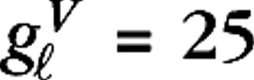 cd−1 m2 s−1. The LGN kernels are of the form (Benardete and Kaplan 1999)
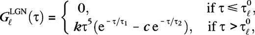
 and
and  are the center and surround sizes, respectively, and
  is the integrated surround–center sensitivity. The temporal kernels are normalized in Fourier space,
 For the magno cases (M0, M10), the time constants τ1 = 2.5 ms, τ2 = 7.5 ms, and c = (τ1/τ2)6 so that
  in agreement with experiment (Benardete and Kaplan 1999). For the parvo cases (P0, P10), the time constants τ1 = 8 ms, τ2 = 9 ms, and c = 0.7(τ1/τ2)5. The delay times
  are taken from a uniform distribution between 20 and 30 ms, for all cases. Sizes for center and surround were taken from the experimental data (Hicks and others 1983; Derrington and Lennie 1984; Spear and others 1984; Shapley 1990; Croner and Kaplan 1995) and were
  0.2°, 0.04°, 0.0875° (centers) and
  1.4°, 0.32°, 0.7° (surrounds), for M0, M10, P0, and P10, respectively. The integrated surround–center sensitivity was in all cases
  (Croner and Kaplan 1995). By design, no diversity has been introduced in the center and surround sizes in order to demonstrate the level of diversity resulting purely from the cortical interactions and the connection specificity between LGN cells and cortical cells (i.e., the sets see specifications below). Further, no distinction was made between ON-center and OFF-center LGN cells other than the sign reversal of their receptive fields (± sign in eq. 6). The LGN receptive field centers
  were organized on a square lattice with lattice constants σc/2, σc, σc/2, and σc/2 for M0, M10, P0, and P10, respectively. These lattice spacings and consequent LGN receptive field densities imply LGN cellular magnification factors that are in the range of the experimental data available for macaques (Conolly and van Essen 1984; Malpeli and others 1996). The connection structure between LGN cells and cortical cells, given by the sets is made so as to establish ocular dominance bands and a slight orientation preference, which is organized in pinwheels (Blasdel 1992). It is further constructed under the constraint that the LGN axonal arbor sizes in V1 do not exceed the anatomically established values of 1.2 mm for magno and 0.6 mm for parvo cells (Blasdel and Lund 1983; Freund and others 1989). A sketch of the model is given in Figure 1. Further details are provided in Supplementary Materials.
Some of the geometric differences between the different model configurations can be expressed by the dimensionless parameter  where v−1 is the cortical magnification factor, σc is the LGN receptive field size (center size), and
  is a characteristic length scale for the excitatory cortical connectivity. Substituting numerical values taken from the experimental data, this parameter is 1, 0.57, 0.4, and 0.25 for M0, M10, P0, and P10, respectively. At 30° eccentricity, the experimental data suggest values for this parameter not very different from its values at 10° (Ω = 0.5 for M30 and Ω = 0.25 for P30).
In the construction of the model, our objective has been to keep the parameters deterministic and uniform as much as possible. This enhances the transparency of the model while at the same time provides insight into what factors may be essential for the considerable diversity observed in the responses of V1 cells. Important parameters which are not subject to cell-specific variability are
Parameters related to the integrate-and-fire mechanism, such as threshold, reset voltage, and leakage conductance. These are identical for all cells (eq. 1).
The cortical interaction strengths and connectivity length scales. These are presented by the functions which are not cell specific but only specific with respect to the 4 cell populations. Note: the functions are also not configuration specific (eq. 3).
Maintained activity and responsiveness to visual stimulation of LGN cells (eq. 4).
Receptive field sizes of LGN cells. These are neither cell nor population specific (i.e., where “population” in this case refers to the ON and OFF LGN cell populations) but are only specific with respect to the 4 model configurations, that is, receptive field sizes of all LGN cells are identical for a particular configuration (eq. 6).
Important model parameters which are subject to a cell-specific variability are
The external noisy conductances ηE,i(t) (excitatory) and ηI,i(t) (inhibitory) (eq. 2).
The cortical synaptic dynamics as described by the kernels Gμ,j(τ) (eq. 3).
The LGN temporal kernels
 (eq. 4).
The LGN connectivity to our model cortex as described by and (eq. 4).
Visual Stimuli and Data Collection
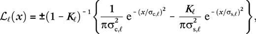
The stimulus used in this paper to analyze surround suppression and contrast-dependent receptive field size is a drifting grating confined to a circular aperture, surrounded by a blank (mean luminance) background. The luminance of the stimulus is given by  for
for  and
and  for
for  with average luminance I0, contrast ε, temporal frequency ω, spatial wave vector
  and aperture radius rA. The aperture is centered on the receptive field of the cell and varied in size, whereas the other parameters are kept fixed at close to preferred values for the cell. The stimuli are presented monocularly (other eye I = 0). As the aperture size increases, the response of a real V1 cell to such stimuli typically reaches a maximum, after which it settles down to a steady level.
The primary data in this paper, that is, responses and conductances as a function of aperture size for monocular stimulation, are obtained with the temporal and spatial frequencies of the grating set equal to the averaged preferred values for each model configuration (M0, M10, P0, and P10). Data used for analysis are from cells that have their preferred orientation equal to the grating angle, their preferred temporal frequency within 2 Hz of the grating frequency, a preferred spatial frequency kp that satisfies where k is the grating spatial frequency, a receptive field center that is less than 1/20th of the average receptive field size away from the aperture center, a maximum response at low contrast that is greater than fb + 5 where fb is the mean blank response (in spikes per second), and, finally, a central cortical location confined to the dashed white rectangle in Figure 1. Samples consist of approximately 200 cells, with about equal numbers of simple and complex cells. Each stimulus was presented for 3 s and preceded by a 1 s blank stimulus. The procedure was repeated five times with different initial conditions and noise realizations. Standard errors in cycle-trial average responses and conductances are negligible. The experiments were performed at “high” contrast, ε = 1, and “low” contrast, ε = 0.3. Additional details are provided in Supplementary Materials.
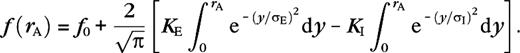
Difference-of-Gaussians and Ratio-of-Gaussians Models
As is true for SI1, SI2 can be greater than one, indicating surround suppression beyond the background response. The limitations of the DOG model can be made more apparent by noting that, given the validity of the half-wave rectification model equation (13), one “derives” the DOG model by the substitutions
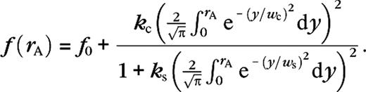
As for the DOG model, the limitations of the ROG model can be made more apparent by noting that, from equation (12), it may be “derived” from the standard half-wave rectification model. Equation (12) can be rewritten such that the numerator (N) and the denominator (D) represent a half-wave rectified weighted difference of the excitatory and inhibitory conductances, and the total conductance gT, respectively. The ROG model used in Cavanaugh and others (2002) is then obtained by the substitutions
Results
Classical Response Properties
One of our model's strong accomplishments is that it produces, with the same fixed parameters, a variety of response properties in good agreement with the experimental data. It also displays a great diversity in each of its response properties, quite similar to what is seen experimentally. Cells in the model exhibit in addition to the 2 extraclassical response properties central in this paper many realistic “classical response properties.” By this we mean response properties, such as orientation tuning, spatial and temporal frequency tuning, and response modulations for drifting and contrast reversal grating stimuli, obtained for large, homogeneous (grating) stimuli, so that size effects of the stimulus are no longer observable. Our motivation for referring to these properties as “classical” stems from the fact that this is how they are traditionally obtained, that is, with use of large homogeneous stimuli. Classical response properties generally show modest changes when the stimuli are confined to the classical receptive field. These changes, in fact, form an interesting class of extraclassical response properties by themselves, of which surround suppression, as defined in this paper, is just 1 example. The classical receptive field is approximately equivalent to the minimum response field (Hubel and Wiesel 1962; Henry and others 1978; Gilbert 1997) and is precisely defined in Methods. Throughout this paper, we will refer to the classical receptive field simply as the receptive field.
Classical response properties are important when considering extraclassical phenomena. One of the reasons is that extraclassical phenomena are evoked from outside the receptive field but are not known to occur without sufficient stimulation of the receptive field. Extraclassical responses are thus defined relative to responses from within the receptive field, or equivalently, relative to classical responses. For example, consider orientation tuning. A cell's orientation-tuning curve obtained for a large, homogeneous grating (classical response property) will, in general, be modestly different from its tuning curve obtained when the same grating is confined to the receptive field. In general, there will be an overall increase in response and orientation selectivity will be somewhat less for the latter stimulus, whereas the preferred orientation will remain the same. Differences between the cell's orientation tuning for the 2 stimuli are precisely what constitute the extraclassical response properties (phenomena) in this case. It would therefore be less meaningful to present an analysis of extraclassical receptive field phenomena based on a cell population of a model if the basic classical responses for that cell population are nonexistent or show poor agreement with the experimental data.
Another reason for the importance of classical response properties is that responses of cortical cells depend strongly on how the cell's environment is responding. The responses of the cells that make up this environment will, in general, display an enormous diversity to any particular fixed stimulus. A cell's cortical environment generally consists of cells that have vastly different orientation and spatial and temporal frequency tuning widths and preferences. The fact that our model's classical responses, including their diversity, agree well with the experimental data thus provides some guarantee for a reasonable response of a cell's environment, not only for classical stimuli but, more importantly perhaps, also for extraclassical stimuli.
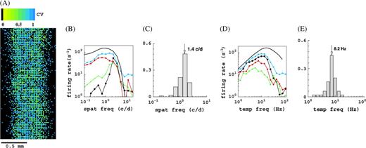
Select classical response properties of the M0 version of the model, other configurations yield similar results. (A) Spatial distribution of orientation selectivity, expressed in the CV (color coded), for cells within the white rectangle in Figure 1. Black pixels are cells that do not show sufficient response for this monocular stimulation. (B) Spatial frequency tuning curves for select M0 cells. Thick black curve refers to the LGN cells, which are all identical in this respect. (C) Distribution of preferred spatial frequencies for the M0 cells. (D) Temporal frequency tuning curves of some M0 cells. Thick black curves refer to the LGN cells, which are all identical in this respect. (E) Distribution of preferred temporal frequencies for the M0 cells. Histograms show fraction of cells, and the arrow indicates mean value.
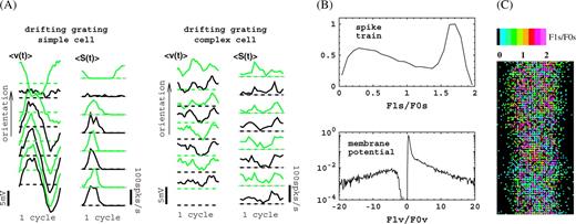
Response modulations in the model for (large) drifting grating stimuli with average optimal spatial and temporal frequency of the cortical cells. (A) Response waveforms for a simple and a complex cell, with optimal spatial and temporal frequencies close to the grating values, for a number of different grating orientations (angles) running form 0 to 7π/8. (B) Distributions (normalized to peak value 1) of F1s/F0s for spike responses and F1v/F0v for membrane potential responses. (C) Spatial distribution of F1s/F0s (spike train) for cells within the white rectangle in Figure 1. Black pixels are cells that do not show sufficient response for this monocular stimulation. For sample selection and additional details, see Supplementary Materials.
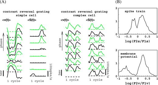
Response modulations in the model for (large) standing grating (contrast reversal) stimuli with the average optimal spatial and temporal frequency of the cortical cells. (A) Response waveforms for a simple and a complex cell with preferred orientation, optimal spatial and temporal frequencies, close to the grating values, for a number of different spatial phases ψ. (B) Distributions (normalized to unity) of the phase-averaged F2s/F1s ratio for spike train (top) and F2v/F1v for membrane potential (bottom) responses to a contrast reversal grating at the preferred orientation. Sample contained 1200 cells. For sample selection and additional details, see Supplementary Materials.
Here r(θ) is the mean firing rate and θ the orientation. Smaller CV indicates a higher orientation selectivity. Cells with CV = 0 respond at just 1 orientation and hence are very selective (sharply tuned). Cells with CV = 1 respond identically at all orientations and hence are not selective for orientation. In Figure 2A, we color coded the CV for all cells within the white dashed rectangle in Figure 1. The stimulus (drifting grating) was presented monocularly; the other eye received no visual input. Pixels colored black indicate cells that do not show a significant response for this monocular stimulation and are mostly cells that respond to stimulation of the other eye. Notice that our model cortex is filled with very selective cells, moderately selective cells, and nonselective cells, as is the primary visual cortex of macaques. Notice also that there is no particular spatial organization of orientation selectivity in our model. Our model yields a diversity in spatial and temporal frequency tuning properties that is quite similar to what is observed experimentally. This is illustrated in Figure 2B–E. In considering this diversity, it is important to note that, in this respect, all LGN cells in a particular configuration are identical by construction. Their spatio-temporal tuning properties are indicated by the thick black curves. As in reality, the preferred temporal frequencies of our cortical cells are lower than the preferred temporal frequency of our LGN cells. The main reason for this is the inclusion of slow, N-methyl-𝒟-aspartate, excitation in the model (Krukowski and Miller 2001) (see also Supplementary Materials). The diversity seen in the spatial frequency tuning of our cortical cells, when compared with the LGN cells, originates in part from the spatial diversity in the feed-forward LGN connections. However, by far the largest contributions, particularly for what concerns the increase in selectivity (sharpening), are cortical in origin. That is, the spatial frequency selectivity of the LGN inputs gLGN is substantially sharpened by the cortical interactions, similar to the sharpening of orientation selectivity as explained in McLaughlin and others (2000).
A partial list of the sources of variability (and of invariability) in the model's construction is given in Methods. In observing the diversity of responses in our model, however, one should also bear in mind that our model is a high-dimensional (many dynamic variables, i.e., vi(t) and 𝒮i(t)) nonlinear system. The behavior of such systems is almost by definition nontrivial. Note in this respect, for instance, that the cortical interaction term, equation (3), contains the dynamic variables 𝒮i(t). This means that, although some diversity may have been introduced in the construction of the model (LGN connectivity for instance), it is not correct to conclude that therefore the diversity observed in the model's response would simply be a direct reflection of that diversity. Because of the dynamic variables 𝒮i(t), diversity (and in fact, by far the largest) is also introduced by the dynamics of the model. A good example of this, and at the same time of the nontrivial behavior of such large systems, is orientation tuning. As can be seen in Figure 2A, the system displays a large diversity for orientation tuning, attaining a CV anywhere between 0 and 1. If one considers the CV in our model without the cortical interactions, however, one finds that now there is practically no orientation tuning or diversity, CV's range anywhere between 0.8 and 1. Thus, the diversity introduced, by construction, in the LGN connectivity provides by itself little diversity in orientation tuning because the CV as a result of these inputs alone is always greater than 0.8 (and less than 1). The diversity of orientation tuning in the model is thus largely dynamical in origin and due to the cortical interactions, that is, to the dynamics of these interactions. We cannot discuss such issues in too much detail as it would lead us away from the main points. A nice demonstration of the above example, however, can be found in McLaughlin and others (2000). In that paper, the diversity in orientation tuning generated by the cortical interactions is shown explicitly, with practically no diversity in the LGN connectivity.
Another example of classical response properties of the model is provided in Figure 3. Shown in Figure 3A are averaged response waveforms of spike train and membrane potential in response to a drifting grating. These are responses of a simple and a complex cell, for several grating orientations, at the cells' preferred spatial and temporal frequencies. The modulation in the spike train at the preferred orientation is frequently used to classify simple and complex cells in V1. A cell is “complex” whenever F1s/F0s < 1 and “simple” otherwise, where F1s is the first harmonic of the spike response and F0s the mean. The distribution of F1s/F0s over a cell population is shown in Figure 3B (top). Our model contains about an equal number of simple and complex cells. The bimodal shape of the distribution of F1s/F0s agrees well with the experimental data (Ringach and others 2002). In fact, the availability of this distribution provided us with a useful criterion for setting the cortical interaction strength parameters in the model (see Supplementary Materials for details).
It is easy to understand the origins of the diversity in response modulations in our model. The modulations enter our model cortex via the LGN input, which targets 30% of the cortical cells. The phases of these LGN inputs vary randomly (approximately uniform distribution) on [0, 2π]. This is due to the receptive field offsets of the clusters of LGN cells connected to different cortical cells, the difference in shape (symmetry) of the clusters themselves, and the diversity in temporal delays in the LGN kernels. A cell receives input from many other cells, thus a cell's excitatory and inhibitory inputs will show stronger or weaker modulations depending on its specific environment in the network and whether or not it receives LGN input. Interplay between the strengths and phases of the modulations in these inputs ultimately determine the modulation in the cell's firing rate and membrane potential. Most cells that receive LGN input are simple cells (80% in our model), and most cells that do not receive LGN input are complex (70% in our model).
The distribution of the subthreshold modulation ratio F1v/F0v, where the membrane potential is measured with respect to a blank stimulus, is shown in Figure 3B (bottom). Notice that the bimodality we observe in the distribution of F1s/F0s is not present in the distribution of F1v/F0v. However, we find that (not shown) the classification of simple and complex cells can be equally well made in terms of the distribution of F1v/F0v, the 2 modes in this case being its “core” (|F1v/F0v|<2, complex cells) and its “tails” (|F1v/F0v|>2, simple cells). Also notice that we observe a “gap” in the distribution at small negative values. Details regarding the F1v/F0v distribution for our model will be published in a separate note. The distribution of modulations in the membrane potential has not yet been observed experimentally for macaques. Some data for cats have recently been published (Priebe and others 2004), and they do not contradict the predictions based on our model. The spatial distribution of F1s/F0s (spike train) across all cells within the white dashed rectangle in Figure 1 is shown in Figure 3C. Once again, the stimulus was presented monocularly, and pixels colored black indicate cells that do not show a significant response for this stimulation. The figure shows that simple and complex cells are randomly distributed across our model cortex, that is, there is no particular spatial organization of F1s/F0s.
A final example of classical response properties of our model is provided in Figure 4. Averaged response waveforms of spike train and membrane potential in response to a standing (contrast reversal) grating  at the preferred orientation are shown in Figure 4A. Shown are the responses of a simple and a complex cell in the model for several spatial phases ψ of the grating. Simple cells perform an approximately linear spatial summation, that is, their responses contain a dominant first harmonic (F1s, F1v), and the spatial phase dependence of their response waveform is similar to the spatial phase dependence of the magnitude of the intensity modulations of the stimulus at any given fixed position. Complex cells respond nonlinearly, and their response waveform is relatively insensitive to spatial phase and contains a dominant second harmonic (F2s, F2v). The distribution of the ratio of second to first harmonic of the response, averaged over the spatial phase ψ, is shown in Figure 4B. For what concerns the spike train waveforms (top), the distribution of F2s/F1s displays a weak bimodality and its behavior for our model cells agrees with the experimental data (Hawken and Parker 1987), complex cells having mostly F2s/F1s > 1 and simple cells F2s/F1s < 1. Note that this property of our model cells follows naturally, without any parameter adjustments, after the strength parameters have been set to achieve essentially only orientation tuning and a proper distribution of response modulations in response to a drifting grating (Fig. 3B, see also Wielaard and others 2001).
It is easy to understand the origins of the diversity in F2s/F1s (and F2v/F1v) in the model. As explained in Wielaard and others (2001), for a contrast reversal grating stimulus, each total LGN input into a cortical cell has, in general, a dominant first harmonic with a phase close to either 0 or π, determined by the relative positions of the ON and OFF subfields of the corresponding cluster. The cortical excitatory and inhibitory inputs in a cell will thus have a relatively strong second harmonic component because they arise from many other cells. The actual strengths of first and second harmonic in a cell's excitatory and inhibitory inputs thus depend on the cell's specific environment in the network and on whether it receives LGN input or not. Interplay of these inputs determines the ratios of first to second harmonic in the cell's spike and membrane potential responses. Clearly, most cells that receive LGN input (simple) will have F2s/F1s, F2v/F1v < 1 and most cells that do not receive LGN input (complex) will have F2s/F1s, F2v/F1v > 1.
No experimental data are available for the distribution of F2v/F1v of the membrane potential waveforms. The distribution of this quantity (averaged over the spatial phase ψ) for the model is shown in Figure 4B (bottom). Our model predicts that, quite contrary to the situation for F1v/F0v, the (weak) bimodality of the distribution of F2s/F1s for spike waveforms is not eliminated but, rather, becomes more pronounced in the F2v/F1v distribution for membrane potential waveforms. This, in fact, can be understood quite simply from a standard half-wave rectification model, in which the membrane potential waveforms are subjected to a threshold to give the spike waveforms. Specifically, for complex cells, both the membrane potential and spike responses will contain a strong second harmonic component. In this case, practically all of the membrane potential waveform will be above threshold, so that evaluation of F2s/F1s for spike waveforms will yield about the same result as F2v/F1v for membrane potential waveforms. This is also apparent in Figure 4B: the F2s/F1s > 1 and the F2v/F1v > 1 sections of the 2 distributions (in top and bottom panels) are very similar. For simple cells, the membrane potential and spike responses will contain a dominant first harmonic and for both responses about an equally small second harmonic component. Because of the half-wave rectification, the F1v component in the membrane potential waveform is substantially reduced in the spike waveform. Hence, F2v/F1v will turn out substantially smaller than F2s/F1s. This is again apparent in Figure 4B: the F2v/F1v < 1 section (simple cells) of the distribution for membrane potential waveforms (bottom) is markedly shifted to the left with respect to the F2s/F1s < 1 section of the distribution for spike responses (top).
Extraclassical Response Properties
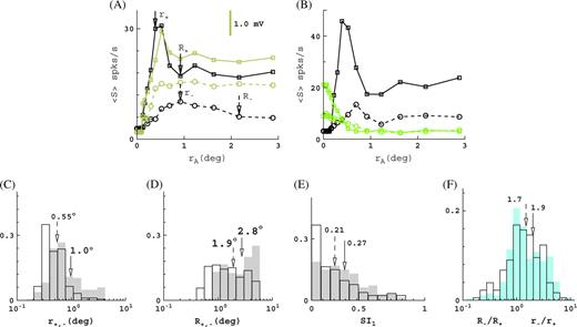
In this section, we summarize the extraclassical results for our model and compare them with the experimental data. Contrary to classical response properties, the 2 extraclassical response properties focused on in this paper are, as for experimental data, not substantially different for simple and complex cells and are therefore not made type specific in what follows. Figure 5A,B shows examples of the surround suppression and receptive field expansion observed in our model. Responses are shown for both firing rate and membrane potential, at high (solid) and low (dashed) contrast.
Summary of surround suppression and receptive field growth at low contrast in the model. (A) Responses (F1s, F1v) as function of aperture size rA for a cell from the M0 model. Shown are firing rate (black) and membrane potential (brown) for high (squares) and low (circles) contrast. Standard errors are negligibly small. (B) Responses (F1s) for another cell from the M0 model. Shown are firing rate as function of the aperture size rA (black) and the response to the inverse stimulus (green), that is, a stimulus where the aperture is “blank” and is surrounded by drifting grating. Responses are again shown at high (solid) and low contrast (dashed). Stimulation solely from outside the cell's receptive field r+,− does not evoke any response, believed to be a signature of extraclassical responses. (C and D) Receptive field and surround sizes for the P10 model at high (unfilled) and low (shaded) contrast. The diversity of responses produced by the model is similar to what is seen in the experimental data (Sceniak and others 2001; Cavanaugh and others 2002). (E) Distribution for the M0 model of the suppression index SI1 at high (unfilled) and low (shaded) contrast. All suppression is exclusively cortical in origin and due solely to short-range connectivity. (F) Distributions for the M0 model of the ratios of the receptive field and surround sizes at low and high contrast, r−/r+ (blue shaded) and R−/R+ (unfilled). (Wilcoxon test on ratio larger than unity: P < 0.001 for both receptive field and surround growth.) In panels (C–F), histograms give fraction of cells, arrows indicate means, solid arrow corresponds to shaded histograms, and dashed arrow corresponds to unfilled histograms. For a more complete summary of our model data, see Supplementary Materials.
Distributions of receptive field and surround sizes for the 4Cβ, 10°-eccentricity model (P10) are shown in Figure 5C,D. The distributions for the other model configurations are given in Supplementary Materials. Receptive field sizes and surround sizes in our model show excellent agreement with the experimental data (Sceniak and others 2001; Cavanaugh and others 2002). This is true for the mean values, for the diversity, as well as for their dependence on eccentricity. Specifically, Figure 3A of Sceniak and others (2001) shows that surround sizes are for about 95% of the cells <4° in radius, with an average surround radius of approximately 2°. Note that Sceniak and others (2001) actually use the inhibitory space constant of the DOG model as a measure of surround radius, though this is a minor detail. Further, Figure 2 of Cavanaugh and others (2002) shows that 100% of the cells have surround radii <6°. Average surround radius at 10° eccentricity is about 2.5°; at para-foveal eccentricities, the average surround radius is 1.25°. In Figure 5A of Levitt and Lund (2002) about 85% of the cells have surround radii <2.5°. Average surround radius is about 1.5°. In Figure 2D of Angelucci and others (2002) about 70% of the cells have surround radii <6°, whereas the average surround radius is 2.5°. We have pointed to the relevant figures from these references for extra clarity, because the precise sizes of the surrounds in V1 are the cause of some ongoing debate.
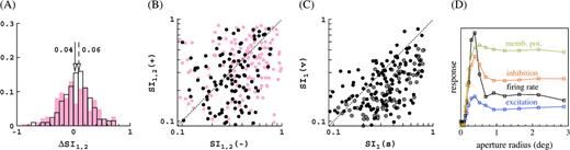
The distribution of surround suppression and receptive field growth for the M0 configuration of our model is given in Figure 5E,F. The suppression index SI1 is defined in Methods. Briefly, it gives the relative suppression: cells without surround suppression have SI1 = 0 and cells with fully suppressed response for large stimuli have SI1 = 1. In agreement with the experimental data, the shape of the distribution of the suppression index SI1 is skewed to low suppression (Cavanaugh and others 2002). Further, in agreement with the experimental data, we observe a small increase in the mean suppression at low contrast (Sceniak and others 1999; Cavanaugh and others 2002). The change in suppression, ΔSI1 = SI1(−) − SI1(+), is broadly distributed (Sceniak and others 1999) around a mean 0.06 (see Figure 6A,B). The average suppression index (over all eccentricities) is SI1 ∼ 0.2, and this is about half of what is observed experimentally (Cavanaugh and others 2002). The receptive field and surround growths (Fig. 5F) are expressed as ratios, r−/r+ and R−/R+, respectively. The indices + and − refer to high and low contrast, respectively. We observe an average growth by about a factor of 2 in both receptive field size and surround size This receptive field growth is a little less than what is observed in experiments (Kapadia and others 1999; Cavanaugh and others 2002).
Relations between some key response measures for the M0 configuration of the model, other cases yield qualitatively similar results. (A) Distribution of the change in the suppression index with contrast, ΔSI1, 2 = SI1, 2(−) − SI1, 2(+), for the suppression indices used in Cavanaugh and others (2002) (SI1, unfilled histogram) and in Sceniak and others (1999) (SI2, pink-shaded histograms). Histograms give fraction of cells, arrows indicate means, solid arrow corresponds to shaded histogram, and dashed arrow corresponds to unfilled histogram. (B) Scatter plot of surround suppression at low and high contrast expressed in the 2 different suppression indices SI1 (black) and SI2 (pink). (C) Scatter plot of surround suppression in spike train and membrane potential at high (black) and low (gray) contrast. (D) First harmonic (F1) of spike responses, membrane potential responses, and cortical conductances as function of aperture size for a model simple cell that shows about 50% surround suppression (in spike train). Notice the surround suppression of the conductances.
We also fitted our data with the DOG and ROG (Sceniak and others 1999; Cavanaugh and others 2002) models (Methods). We obtain for the integrated suppression index SI2 ∼ 0.4. Average growth ratio for the excitatory space constant is (both DOG and ROG, averaged over all eccentricities). Again, in agreement with the experimental data (Sceniak and others 1999), we observe a small increase in the mean suppression at low contrast, and the change in suppression, ΔSI2 = SI2(−) − SI2(+), is broadly distributed around a mean 0.04 (see Figure 6A,B). The suppression index and growth ratio are again less than those experimentally observed (0.6 and 2.3, respectively; Sceniak and others 1999).
All the above findings are based on spike responses. Membrane potential responses yield qualitatively similar results, but due to the spike threshold, suppression in the membrane potential is systematically smaller. This is illustrated in Figure 6C. The same observation has also been made experimentally in cats (Anderson and others 2001). A more extensive summary of the data generated by our model data, for different eccentricities and including receptive field sizes and surround sizes, is given in Supplementary Materials.
Mechanisms of Surround Suppression
The DOG and ROG models are phenomenological models and provide limited insight into the neural mechanisms of the phenomena. Both models miss an essential feature of the excitatory and inhibitory inputs, which is that these inputs generally show surround suppression themselves (Anderson and others 2001). In our model, we similarly observe a significant suppression in both conductances, as shown in Figure 6D. This cell shows that, unlike what is suggested by the DOG and ROG models, surround suppression in the spike response takes place entirely in the region of decreasing synaptic inputs (conductances). We can say that the surround suppression of this cell is caused by a decrease of excitation because the decrease of inhibition could not by itself suppress the cell's response. This cell is not uncommon in our model, and the above scenario is indeed how surround suppression works in about 50% of the cells.

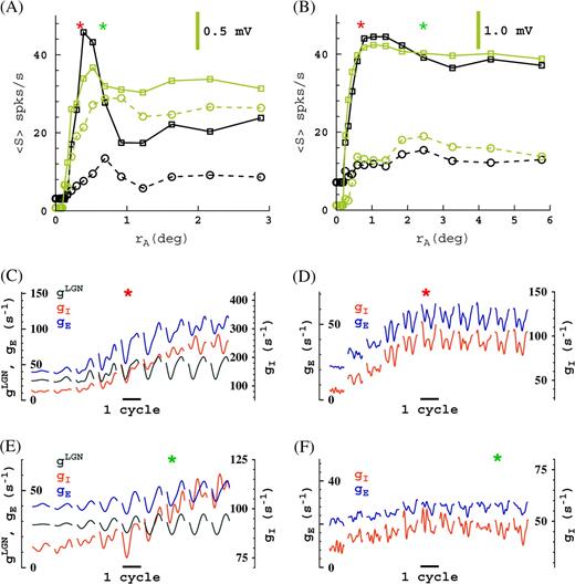
Examples of this analysis for a (simple) cell receiving LGN input and a (complex) cell that does not receive LGN input are given in Figure 7. The cycle-trial–averaged conductances for consecutive apertures around the aperture of maximum response (rA = r, marked by an asterisk) are shown in Figure 7C–F. For example, by comparing the conductances for aperture “asterisk” and the aperture for which the suppression is maximum (rA = R, for instance, the third aperture to the right of aperture asterisk in Fig. 7C), we see that at high contrast the suppression mechanism for the simple cell (Fig. 7C) is (A) and for the complex cell (Fig. 7D) is (B). At low contrast the suppression mechanisms are (C) and (B) (Fig. 7E,F, respectively).
Two example cells, an M0 simple cell that receives LGN input (left) and an M10 complex cell that does not receive LGN input (right). (A and B) Responses as functions of aperture size. Mean responses (firing rate and membrane potential) are plotted for the complex cell, and first harmonic for the simple cell. Apertures of maximum of responses (i.e., receptive field sizes, rA = r) are indicated with asterisks, red = high contrast, green = low contrast. (C and D) Conductances for high contrast at consecutive apertures near the maximum responses. (E and F) Conductances for low contrast at consecutive apertures near the maximum responses. Panels (C and E) each consist of 9 subpanels, panels (D and F) each consist of 11 subpanels, giving the cycle-trial averaged conductances as function of time (relative to cycle) and aperture size. Asterisks indicate corresponding apertures of maximum response in (A and B).
We observe all 3 mechanisms (A, B, and C) in our model. By comparing the responses and conductances for apertures from the receptive field size rA = r to the surround size rA = R, we can identify the suppression sequence, that is, the mechanisms that act sequentially as the aperture size rA increases from receptive field size r to surround size R. We observe a rich variety of suppression sequences in the model. In some cases, we find that different mechanisms are active during different times in the stimulus cycle.
As may be clear from Figure 7, identifying the mechanisms for surround suppression based on equations (12) and (13) can be rather more subtle than just comparing the mean (F0) conductance, its first harmonic (F1), or the peak conductance (∼F0 + F1). However, we find that for most cells, an analysis using the sum of first and second harmonic (F0 + F1) of the conductances allows the identification of the suppression mechanisms. Comparing conductances at rA = r and at rA = R in this way, we find that at low contrast all 3 mechanisms are about equally prevalent, whereas at high-contrast mechanism (A) is somewhat more likely than (B) and (C).
Mechanisms of Receptive Field Expansion
The DOG model suggests that receptive field growth at low contrast is due to an increase of the spatial summation extent of excitation (Sceniak and others 1999) (for our data, correlation coefficient between r−/r+ and is r = 0.55, correlation coefficient between r−/r+ and is r = 0.17). This was partially confirmed experimentally in cat's primary visual cortex (Anderson and others 2001). Although it has been claimed (Cavanaugh and others 2002) that the ROG model would explain receptive field growth solely from a change in the relative gain parameter ks, we believe this is incorrect. Because there is a one-to-one relation between ks and the surround suppression, this would imply that receptive field growth (increase) at low contrast simply results from contrast-dependent (decrease) surround suppression, which contradicts the experimental data (Sceniak and others 1999; Cavanaugh and others 2002). As does the DOG model, the ROG model, based on analysis of our data, also predicts that receptive field growth at low contrast is due to a growth of the spatial summation extent of excitation at low contrast. As we will now show, our simulations do confirm an average growth of spatial summation extent of excitation (and inhibition) at low contrast, but this growth is neither sufficient nor necessary to explain receptive field growth.
A change in the spatial summation extent of gE and/or gI is just one of the many ways to change the behavior of G and consequently the receptive field size. For example, some other possibilities are illustrated by the 2 cells in Figure 7. These cells show, both in spike and membrane potential responses, a receptive field growth of a factor of 2 (left) and 3 (right) at low contrast. However, for both cells, the spatial summation extent of excitation at low contrast is 1 aperture less than at high contrast.
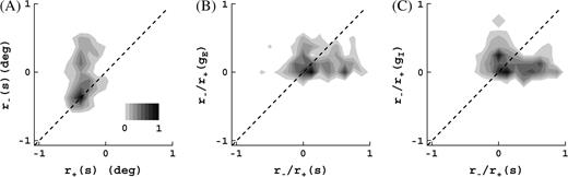
The receptive field expansion at low contrast is apparent in Figure 8A. In agreement with the experiment (Sceniak and others 1999; Cavanaugh and others 2002), we observe little correlation between this growth and the surround suppression (correlation coefficient between r−/r+ and ΔSI1 is r = 0.01). In a similar way as for spike train responses, we obtained receptive field sizes for the conductances. As shown in Figure 8B,C, both excitation and inhibition also show, on the average, an increase in their spatial summation extent as contrast is decreased. This increase is, however, rather arbitrary and bears not much relation with the receptive field growth based on spike responses (correlation coefficient between r−/r+(s) and r−/r+(gE) is r = 0.06, between r−/r+(s) and r−/r+(gI) is r = 0.07, between r−/r+(gE) and r−/r+(gI) is r = 0.1). Further, the increase is, in general, smaller than what is seen for spike responses, particularly for cells that show significant receptive field growth. For instance, we see from Figure 8B,C that for cells with receptive field growth ∼2 and greater the growth for the conductances is always considerably less than the growth based on spike responses. Expressed more rigorously, a Wilcoxon test on ratio of growth ratios larger than unity gives P < 0.05 (all cells, excitation, Fig. 8B), P < 0.15 (all cells, inhibition, Fig. 8C), and P < 0.001 (cells with receptive field growth rate r−/r+ > 1.5, both excitation and inhibition). Similar conclusions follow from membrane potential responses (not shown).
(A) Joint distribution of high- and low-contrast receptive field sizes, r+ and r−, based on spike responses. All scales are logarithmic (base 10). All distributions are normalized to peak value 1. Receptive field growth at low contrast is clear. Average growth ratio is 1.9 and is significantly greater than unity (Wilcoxon test, P < 0.001). (B and C) Joint distributions of receptive field growth and growth of spatial summation extent of excitation (B) and inhibition (C) (computed as ratios). There is practically no correlation between receptive field growth and the growth of the spatial summation extent of excitatory or inhibitory inputs (see text). For cells in the sample with larger receptive field growth (factor of ∼2 and greater), this growth is always considerably larger than the growth of their excitatory and inhibitory inputs.
For cells with significant receptive field growth (r−/r+ > 1.5), we are able to identify additional properties of the mechanisms of the receptive field expansion. For instance, we find that for more than 50% of such cells, a transition takes place from a high-contrast receptive field size less or equal to the spatial summation extent of excitation and inhibition to a low-contrast receptive field size which exceeds both. Details of this analysis are given in Supplementary Materials.
LGN Contributions
The extraclassical responses in our model discussed so far are, by construction, exclusively the result of cortical interactions and not inherited from LGN inputs. This is due to our use of the standard center–surround model for LGN receptive fields (Methods). Our simulations so far have shown that the cortical contributions to surround suppression and receptive field growth can account for a large fraction, but not all, of the magnitude of the phenomena observed experimentally. This leaves room for contributions from the LGN.
It seems reasonable to assume that LGN cells in macaques will display both extraclassical phenomena. Somewhat surprisingly this has to our knowledge not actually been verified yet. Extraclassical surround suppression of LGN cells (at average cortical optimal spatial frequencies) has been observed in marmosets (Solomon and others 2002) and cats (Ozeki and others 2004). Contrast-dependent receptive field growth of LGN cells has been observed in marmosets and an average growth ratio of 1.3 was reported (Solomon and others 2002).
As observed experimentally, the optimal spatial frequency of the LGN cells in our model is substantially smaller than the average optimal spatial frequency kC of the cortical cells (see Fig. 2B). This is why, although our model LGN cells of course do show surround suppression at their optimal spatial frequency, they do not show surround suppression at the higher cortically optimal spatial frequency kC. This is illustrated in Figure 9A. Plotted is the response (gCS) of a single LGN cell as function of aperture size for gratings of different spatial frequencies k. No suppression occurs for k = kC. Suppression starts at spatial frequencies of about 0.5kC. It becomes stronger for smaller spatial frequencies and is 17% at 0.25kC. Further, we find (not shown) that at 0.25kC the surround is not yet able to evoke responses on its own, and the suppression thus in some sense qualifies as “extraclassical.” By lowering the spatial frequency of the stimulus, our model thus enables us to study the transfer of LGN surround suppression to cortical cells.
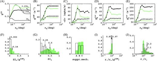
Transfer of LGN surround suppression to cortical cells. (A) Responses of the P10 model LGN cells as function of aperture size, at different spatial frequencies (peak values, relative to response at k = kC). Recall that all LGN cells in a particular model configuration are identical in this respect (Methods). The LGN cells show no surround suppression at the average cortically preferred spatial frequency kC (thick black). The LGN cells show 17% surround suppression at a spatial frequency k = 0.25kC (green). (B–E) Conductances and spike responses for a P10 cortical cell as function of aperture size, for a grating with k = kC (black) and k = 0.25kC (green), at high (solid) and low (dashed) contrast. The LGN conductance gLGN arises from 17 LGN cells for this particular cortical cell. Notice the suppression in gLGN at k = 0.25kC which is absent at k = kC. We see an increase in surround suppression at k = 0.25kC, both in the firing rate 〈S〉 (panel C) and the excitatory cortical conductance gE (panel D) as a result of the suppression in gLGN. Surround suppression in the inhibitory conductance gI (panel E) in general also increases at k = 0.25kC but not for this particular cell. Sum of first and second harmonic (F0 + F1) is plotted for the conductances, and first harmonic is plotted for the firing rate. Unfilled histograms correspond to k = kC, shaded histograms to k = 0.25kC. (F) Distributions of the suppression index of LGN inputs gLGN. (G) Distributions of the suppression index for spike responses of cortical cells in the model. (H) Prevalence of the suppression mechanisms in the model. (I) Distributions of the ratio of spatial summation extent at high and low contrast of LGN input gLGN. (J) Distributions of receptive field growth of cortical cells in the model based on spike responses. Histograms give fractions of cells, arrows indicate means, solid arrow corresponds to shaded histogram, and dashed arrow corresponds to unfilled histogram.
According to Hubel and Wiesel (1962), LGN input arrives in a V1 cell essentially as output of small clusters of about 10–20 LGN cells. Therefore, it is not immediately clear if, and how much of, the surround suppression of the LGN cells is transferred to V1 cells. Our model is constructed to be consistent with the Hubel and Wiesel view (Methods), and the total conductance gLGN (eq. 4) of the cluster of LGN cells feeding into a particular cortical cell is shown in Figure 9B. Plotted are the sum of first and second harmonic (F0 + F1) of gLGN, as a function of aperture size for a grating frequency k = kC (red curves) and k = 0.25kC (blue curves) at high and low contrast. The cell's spike response and cortical excitatory and inhibitory conductances are plotted in Figure 9C,D,E, respectively.
From Figure 9B we see that, other than for the suppression, the behavior of the LGN conductance gLGN is not very different for gratings with k = kC and k = 0.25kC. In particular, its behavior up to its peak value is practically unaltered. This is true in general.
It is important to realize that, in the model, any change in the stimulus affects V1 solely via the LGN inputs gLGN. Further, all LGN inputs oscillate with the constant grating temporal frequency ω, both at k = kC and at k = 0.25kC. By far the dominant changes in the LGN inputs (which are the summed outputs of 20 or so LGN cells) for k = 0.25kC occur in the F1 components. First, in their amplitudes, which has been addressed in Figure 9A,B. Second, in their relative phases. These phase changes, however, can only have a very minor effect on the surround suppression, which can be seen as follows.
As explained earlier, the phases of the LGN inputs vary stochastically with an approximately uniform distribution on [0, 2π], this is so at k = kC and is not notably different at k = 0.25kC (it is only at stimuli close to the uniformly oscillation stimulus, k = 0, that one would observe notable differences [narrowing] in this distribution). The collective effect of the change in the relative phases of the LGN inputs is thus practically nonexistent.
Indeed, the 4 different model configurations, that is, M0, M10, P0, and P10, have similar distributions of surround suppression, receptive field growth etc., whereas each configuration has very different LGN connection structures (eq. 4), with very different relative phases of the LGN inputs in any 2 particular V1 cells. Yet, each case having a similar (close to uniform) distribution of these phases, our simulations show (Supplementary Materials) that the distributions of surround suppression, receptive field growth, and so on do not differ substantially for the different cases.
Hence, we may conclude that substantial differences in behavior of our model cortex for k = kC and k = 0.25kC must be attributed truly to the presence of the surround suppression of the LGN inputs gLGN. Equivalently, we may conclude that such differences must be attributed to the surround suppression of the LGN cells, rather than to other changes in the behavior of the LGN inputs at k = 0.25kC (small contributions of which cannot of course be entirely ruled out).
Some of the differences induced by the LGN surround suppression are apparent from the responses of the cell in Figure 9B–E. We see that there is a sharp increase in the surround suppression of the spike response (Fig. 9C). For k = kC the suppression mechanism is (C) (reduction of excitation and increase of inhibition), whereas for k = 0.25kC it is (B) (reduction of excitation). We can also identify the suppression sequence, which is, as defined earlier, the sequence of active mechanisms when the aperture size rA increases from receptive field size r to surround size R. It is AB at k = kC, and BB at k = 0.25kC. For this cell, which receives LGN input, the increased suppression is caused directly by the LGN suppression (Fig. 9B) as well as an increase in the suppression of the excitatory cortical conductance (Fig. 9D). This increase in the suppression of the excitatory cortical conductance is itself induced by the suppression of the LGN inputs into the many other cells that together make up the cell's cortical environment. We note that, in general, the LGN suppression also induces an increase in the surround suppression of the inhibitory conductances, although for this particular cell this is not significant (Fig. 9E).
A summary of the difference in surround suppression in the model with and without LGN suppression is given in Figure 9F–H. The surround suppression (averaged over high and low contrast) present in the LGN conductances gLGN at k = kC and k = 0.25kC is shown in Figure 9F. As mentioned earlier, we see that at k = kC the LGN inputs do not exhibit surround suppression. Further, we see (shaded histogram) that the average surround suppression of the LGN inputs gLGN is 14%. The distribution of V1 surround suppression (spike responses, averaged over high and low contrast) with and without contributions from the LGN is shown in Figure 9G. Average surround suppression of the cortical cells has increased from 25% to 50%, due to the presence of LGN surround suppression. As mentioned, the LGN surround suppression affects surround suppression of the cortical cells in 2 ways. First, directly via the LGN input for cells that receive it. Second, via the collective action of these inputs, that is, by the increase of the surround suppression of the cortical excitatory conductances. Consequently, we observe that as a result of the LGN surround suppression, the prevalence of suppression mechanisms for our V1 cells is substantially altered in favor of mechanisms (B) and (C) (which require a reduction of excitation) at the expense of mechanism (A) (increased direct inhibition), as shown in Figure 9H. Given that an average surround suppression of SI1 ∼ 0.4 is observed in macaques (Cavanaugh and others 2002), our simulations show cortical short-range connections together with surround suppression present in LGN cells can, in principle, fully account for the degree of surround suppression seen experimentally.
With respect to the possible transfer of receptive field growth of LGN cells to V1 cortical cells, our simulations seem to indicate a lesser sensitivity than for the transfer of surround suppression. As can be seen from Figure 9G, for k = kC the LGN inputs gLGN do not contribute to receptive field growth of our cortical cells. For k = 0.25kC, the average growth ratio of the LGN inputs gLGN has decreased about 10% from its value for k = kC (Fig. 9I), but there is no obvious effect on the average growth ratio for cortical cells (Fig. 9J). Indeed, our analysis of the mechanisms of surround suppression and receptive field growth based on the conductances is largely insensitive to whether we include the LGN conductance in the excitatory conductance or use only the cortical contribution instead. Further, we find that the observations made earlier on, regarding the neural mechanisms of contrast-dependent receptive field size for k = kC, remain qualitatively valid for k = 0.25kC. Our simulations thus indicate an independence of these mechanisms on the transfer of LGN surround suppression to V1.
Despite the apparent lesser sensitivity for transfer from LGN to V1, receptive field growth of LGN cells in some sense introduces an overall geometric scaling factor on the entire visual input to V1. Though this observation ignores a great many details of course. For instance, the fact that the density of LGN cells (LGN receptive fields) is not known to change with contrast. On the other hand, it seems unlikely that a reasonable receptive field expansion for LGN cells would not be at least partially transferred to V1.
The Cortical Magnification Factor
As mentioned in the Introduction, arguments in favor of involvement of long-range connections and/or extrastriate feedback in extraclassical phenomena are indirect and rely on the cortical magnification factor as a key ingredient. Receptive field size and scatter are systematically ignored. It is argued that surround sizes would be too large to result from local short-range connections. We have already shown that, on the contrary, a neural network model constrained by the basic architecture of the V1 input layers, with only local short-range connections, refutes this argument and exhibits surround sizes similar to what is observed experimentally.
One naturally wonders if, and to what extent, our findings depend on the actual value of the cortical magnification factor. Intuitively, a smaller cortical magnification factor is not beneficial for the role of short-range connections in the creation of extraclassical receptive field phenomena because these connections cover less visual space. However, the minimum amount of visual space covered is set by the receptive field size and scatter.
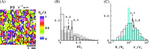
To check whether this minimum visual range of cortical short-range connections is in itself sufficient to generate surround suppression and receptive field expansion, we repeated our simulations with an infinite cortical magnification factor, v−1 = ∞ (geometric parameter Ω = ∞, all else unchanged, see Methods). The results are shown in Figure 10 for the P0 case (M0 yields similar results). Clearly, the finite receptive field scatter by itself, 60% (M0) and 30% (P0) of the average receptive field size (Methods), is sufficient to generate both extraclassical phenomena to practically the same degree as it does in the presence of a realistic cortical magnification factor. Other properties of our model discussed in this paper are also not qualitatively different for infinite cortical magnification factor, with one exception.
As is apparent from Figure 10A, it is now more difficult to connect the LGN cells in such a manner that the organization of orientation preference and ocular dominance displays the same level of order as seen for a realistic cortical magnification factor (Fig. 1). But, this, however, does not imply that order could not be improved with more specific connections.
Results for infinite cortical magnification factor (Ω = ∞) for the P0 configuration, M0 configuration yields similar results. (A) Simulated optical image of ocular dominance and orientation preference, in the spirit of optical imaging experiments (Blasdel 1992) (compare Fig. 1). (B) Distribution of the suppression index SI1 at high (unfilled) and low (shaded) contrast (compare Fig. 5E). (C) Distributions of the receptive field and surround growth ratios, r−/r+ (blue shaded) and R−/R+ (unfilled). Histograms give fractions of cells, arrows indicate means, solid arrow corresponds to shaded histogram, and dashed arrow corresponds to unfilled histogram.
Arguments ruling out local short-range connections and LGN input as the origins of extraclassical phenomena based on the cortical magnification factor are inherently weak because this is a macroscopic measure. Hence, inferences based on it regarding cell–cell influence cannot be very precise. Our simulations further challenge such arguments, by showing that receptive field size and scatter by themselves, regardless of the cortical magnification factor, can be a determinative factor for extraclassical receptive field phenomena.
Discussion
There is considerable debate over the origins of extraclassical receptive field phenomena such as surround suppression and receptive field expansion at low contrast. A primary reason is that it still poses a great challenge for experimental methods to be able to directly distinguish between mechanisms of these phenomena based on local short-range connection, long-range lateral connections, or extrastriate feedback connections. To our knowledge such data are not yet available. This requires that any data regarding the phenomena need to be related to neural mechanisms through some sort of model or theoretical framework. This is not without challenges either. Such a model needs to be sufficiently sophisticated, for example, it needs to cover a large piece of the visual field and cortex, and it needs to adequately address classical response properties because they set the context for the extraclassical phenomena. Ours is an attempt in this direction.
We know of only one other large-scale neural network model in the published literature (Somers and others 1998) that addresses the extraclassical response phenomena discussed in this paper. That model does not address classical response properties, and neural mechanisms for extraclassical phenomena, by construction, arise from long-range connections. Further, in that model, receptive field growth at low contrast is achieved via contrast-dependent surround suppression. That is, the surround suppression systematically decreases as a function of decreasing contrast, which contradicts the experimental data (Sceniak and others 1999; Cavanaugh and others 2002).
We have shown that surround suppression and receptive field expansion at low contrast can be spontaneously generated by short-range cortical connections alone, without any contribution from other sources. We showed that cortical contributions alone, mediated by short-range connections, can explain a major part or the phenomena. We demonstrated that surround suppression of LGN cells, if present, is easily transferred to V1. Our simulations thus provide rigorous computational support for the intriguing hypothesis that the LGN input and cortical short-range connections in V1 are primarily responsible for the surround suppression observed in V1, with little requirement for contributions from long-range or extrastriate connections. We showed that with only 17% suppression in the LGN cells' responses, the cortical surround suppression in the model exceeds the suppression observed experimentally. More radically interpreted, our results therefore would suggest that long-range lateral connections and/or extrastriate feedback, in fact, contribute negatively to surround suppression. That is, rather than being suppressive, our results suggest that their contributions may in fact be facilitatory.
In our model, 3 synaptic cortical mechanisms for surround suppression are active, in agreement with experimental observations in cats (Anderson and others 2001). When LGN suppression is included, we observe strong contributions to cortical suppression from a reduction of recurrent cortical excitation, rather than from an increase in direct cortical inhibition. We find, on average, a growth of spatial summation extent of excitation and inhibition at low contrast, as predicted by DOG (Sceniak and others 1999) and ROG models. But this growth bears no simple relationship with the receptive field growth, neither for superthreshold (spikes) nor for subthreshold (membrane potential) responses. Receptive field growth for these responses usually involves other/additional changes in the relative gain of the excitatory and inhibitory inputs. Notably, significant receptive field growth for these responses is usually much larger than the growth of the spatial summation extent of excitation and inhibition (Fig. 8).
As does the biological primary visual cortex, our model produces these properties in distinctly different geometric settings (with identical strength parameters), namely, for the magno and parvo input layers, at parafoveal eccentricities and around 10° eccentricity. Dimensional observations (parameter Ω) imply that our model results also translate to 30° eccentricity, modulo a geometric scaling factor. The ubiquitous nature of these phenomena and their mechanisms in our model suggest that they are basic response properties of V1. In principle, given realistic classical response properties, they seem to require little more than receptive field scatter and isotropic short-range connectivity, with perhaps some weak constraints on macroscopic organization of ocular dominance and orientation preference. They do not, in principle, seem to require more elaborate architecture or physiological properties, such as specific cortical connectivity, long-range connections within V1, extrastriate feedback, and synaptic depression/facilitation.
Recent data from cats suggest that partial inheritance of surround suppression in V1 from LGN cells does indeed occur (Ozeki and others 2004). Other recent experiments show that strong surround suppression is observed for drifting gratings having spatial and temporal frequencies outside the range at which most cortical cells typically respond, indicating these signals arise within the input layer of V1 or the LGN itself (Webb and others 2004). Given the general nature of our results, we may conclude that the presence of the phenomena in LGN cells could in principle be of the same origin as we have suggested here for V1 cells.
There are further aspects of surround suppression that we have not explicitly addressed in this paper. Among them are orientation tuning of the surround and dynamics (timing) of the suppression. Preliminary simulations indicate that orientation tuning of the surround is well captured by our model. For what concerns timing of the suppression seen in our model, it is clear that through polysynaptic interactions in the network, delays of the onset of surround suppression could range anywhere from 0 to 20 ms, conservatively estimated. Indeed, preliminary simulations show that timing of the surround suppression in our model is consistent with recent experimental findings (Xing and others 2004). Our model has rich dynamics and is well suited to also yield relevant results regarding the dynamics of surround suppression. This is one of our interests for future research.
This work was supported by grants from the Office of Naval Research (MURI program, N00014-01-1-0625) and the National Geospatial-Intelligence Agency (NMA201-02-C0012).