ESPINA: a tool for the automated segmentation and counting of synapses in large stacks of electron microscopy images

Introduction

Chemical axo-dendritic synapses are by far the most common type of synapse in the mammalian brain. Other types of synapses are not found in all regions of the nervous system and when they are present, they are usually only established between specific types of neurons (Peters et al., 1991). The axon terminal has an electron dense thickening on the cytoplasmic face of the pre-synaptic membrane, and close to this pre-synaptic density numerous synaptic vesicles accumulate that are loaded with neurotransmitter molecules. On the opposite side, the inner surface of the post-synaptic membrane also has an electron dense thickening. These pre- and post-synaptic membranes are separated by a narrow gap known as the synaptic cleft. Therefore, the synaptic junction is the complex formed by the pre- and post-synaptic densities and the synaptic cleft (Peters and Palay, 1996). According to their morphology, the synapses in the cerebral cortex can be classified into two main types, Gray’s type I and type II (Gray, 1959), that correspond to the asymmetric and symmetric types of Colonnier, respectively (Colonnier, 1968). In general, asymmetric synapses are considered to be excitatory and much more abundant (75–95% of all neocortical synapses) than symmetric synapses (5–25%), which are inhibitory (for reviews, see Houser et al., 1984; White, 1989; DeFelipe et al., 2002). Therefore, the quantification of synapses, and the identification of the different types and the proportions in which they are found is extraordinarily important in functional terms.

The commonly used stereological methods to quantify synapses are based on the analysis of a limited number of single sections (Sterio, 1984; Colonnier and Beaulieu, 1985) and thus, estimates of the number of synapses per unit volume are very variable and dependent on the sampling methods used in different studies (DeFelipe et al., 1999). To avoid such variability, the ideal approach would be to analyze 3D samples reconstructed from serial sections. However, obtaining serial sections by transmission electron microscopy is an extremely time consuming task that is technically very demanding (Harris et al., 2006; Hoffpauir et al., 2007). Methods have been developed to overcome these difficulties in which serial images are taken from the block face, sequentially removing slices either with a diamond knife (Denk and Horstmann, 2004), or by means of a focused ion beam (FIB) that is used in combination with scanning electron microscopy (SEM; Knott et al., 2008). Using FIB/SEM microscopy, we recently showed that asymmetric and symmetric synapses can be accurately identified, reconstructed, and quantified from large 3D tissue samples, and that virtually all synaptic junctions can be classified regardless of the plane of the section (Merchán-Pérez et al., 2009a). This is important since it has been estimated that approximately 40–60% of the synaptic junctions remain uncharacterized using other techniques (DeFelipe et al., 1999).

In addition, the use of this technique allows long series of sections to be acquired in an automated way, drastically reducing the time necessary to obtain large amounts of data. However, the analysis, segmentation, and quantification of synapses still requires labor intensive user intervention and new solutions must be sought to deal with the large volume of data that is generated by these new automated 3D electron microscopy techniques. The complexity of the information available not only increases due to the amount of images collected but also, because of the type of new data available (e.g., the spatial distribution of objects, their reconstruction and the identification of processes, etc.). When dealing with such complex data, it is essential to design techniques that are specifically adapted to each particular case. This problem, along with the capacity of the human being to analyze and to understand the information visually, has turned the visual representation of information into a highly attractive method. If the problem to which the method is applied is complex, as is the case here, complexity can be depicted in the search process itself as a series of iterative steps that provide tentative solutions to the problem. With regards the analysis of the search process or any interaction with it, the integration of visualization techniques can help improve the quality of the solutions. Furthermore, as mentioned by Fuchs and Hauser (2009), interaction is probably the most important tool to understanding complex data. The interaction process allows us to dynamically modify the visualization parameters, displaying data in such a way that the presence of relevant information is maximized.

There are excellent general purpose software applications that are freely available to aid these tasks, including IMOD (Kremer et al., 1996) or ImageJ (W. Rasband, National Institutes of Health¹) and its distributions especially suited for microscopy (e.g., ImageJ for microscopy: Collins, 2007, and Fiji²). The Reconstruct program (Fiala, 2005) has been especially developed to deal with serial electron microscopy sections, but the accurate reconstruction of synaptic junctions requires manual tracing of the synaptic contours (Arellano et al., 2007; Merchán-Pérez et al., 2009a,b). Other approaches mark-up synaptic junctions instead of rendering their 3D shapes, although this was considered sufficient to tabulate connections in the retina (Anderson et al., 2009). More recently, two promising prototypes to explore and analyze bulky optical and electron microscopy images were described, SSECRETT and NeuroTrace, which reconstruct complex neural circuits of the mammalian nervous system (Jeong et al., 2010). However, no information is available about the distribution policy of these tools. Commercial software such as Amira also have segmentation utilities that could be used for this purpose (Pruggnaller et al., 2008), although none of them address the specific problem of synaptic junction segmentation. Hence, we have developed ESPINA, a software tool that performs automated segmentation and that counts synapses present in a reconstructed 3D volume of the cerebral cortex, greatly accelerating these analyses. The tool is interactive, allowing the user to supervise the process of segmentation, reconstruction, and counting, modifying the appropriate parameters and validating the results. It is also modular, which permits new functions to be implemented as needed. We have also focused on usability, implementing a user friendly interface to minimize the learning curve for the tool, as well as on portability, to make it accessible to a wide range of users.

In the following sections we will describe the capabilities of this software tool together with the data pre-processing required to handle FIB/SEM images with ESPINA.

Tissue Preparation and Serial Section Imaging

Brain tissue from mice and rats was used to develop and test the software. Animals were administered a lethal intraperitoneal injection of sodium pentobarbital (40 mg/kg) and they were intracardially perfused with the fixative. The animals’ brain was then extracted from the skull and processed for electron microscopy (Merchán-Pérez et al., 2009a). All animals were handled in accordance with the guidelines for animal research set out in the European Community Directive 86/609/EEC and all the procedures were approved by the local ethics committee of the Spanish National Research Council (CSIC).

Regions of the neuropil were chosen on the surface of the tissue block for 3D analysis. The 3D study of the brain samples was carried out using a combined FIB/SEM (Crossbeam^® Neon40 EsB, Carl Zeiss NTS GmbH, Oberkochen, Germany). This instrument combines a high resolution field emission SEM column with a focused gallium ion beam which can mill the sample surface, removing thin layers of material on a nanometer scale.

After removing each slice (20 nm of thickness), the milling process was paused and the freshly exposed surface was imaged with a 2-kV acceleration potential using the in-column energy selective backscattered (EsB) electron detector (Figure 1). A 30-μm aperture was used and the retarding potential of the EsB grid was 1500 V. The milling and imaging processes were continuously repeated and long series of images were acquired through a fully automated procedure. For this study, we obtained 2048 × 1536 pixel images, at a resolution of 3.7 nm per pixel, thereby covering an area of 7.577 μm× 5.683 μm before correcting for shrinkage. Under these conditions each milling/imaging cycle took approximately 4 min.

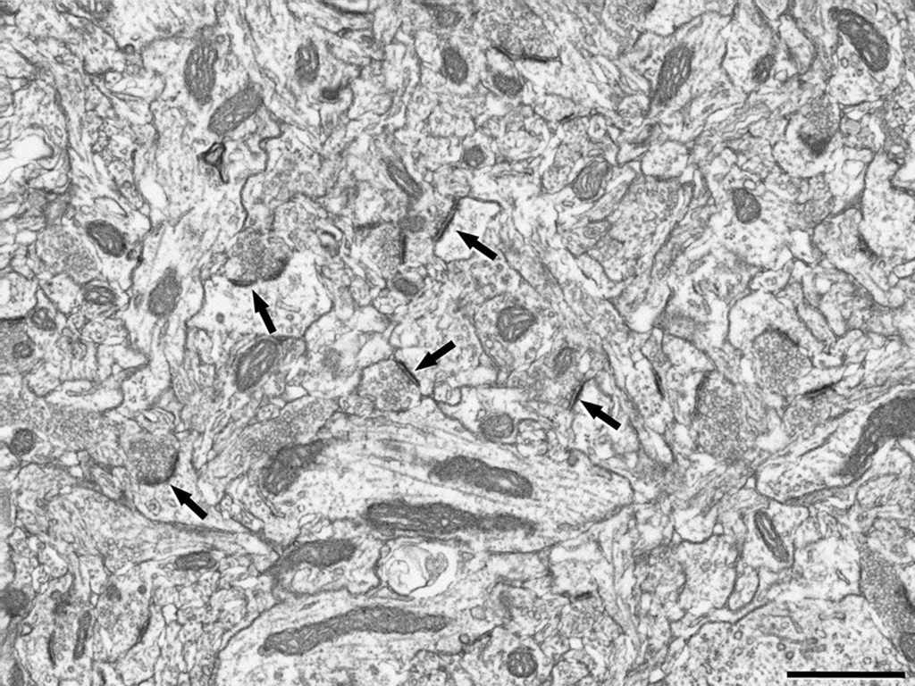
Figure 1. Image captured by focused ion beam milling and scanning electron microscopy (FIB/SEM) showing numerous synapses in the rat cerebral cortex. Some asymmetric synapses are indicated by arrows. Scale bar: 1 μm.

Image Stack Pre-Processing

Alignment (registration) of the stack of images is performed using the stackreg and turboreg plugins of ImageJ (Ph. Thévenaz, école Polytechnique Fédérale de Lausanne³), or with the plugins included with Fiji or any similar application. We apply a rigid registration method (translation only, no rotation) to avoid any deformation of single sections. After registration, the resulting stack must be filtered, cropped, and resized. We use a Gaussian Blur filter with ImageJ to eliminate noisy pixels. Although cropping is not essential, it helps to eliminate undesired margins that may be added during registration, and to select the area to be studied. Finally, resizing is important in order to save computer memory. The use of large samples (currently up to 750 serial sections) is very demanding on memory as a typical series of 250 full size images occupies about 1 GB of disk memory. If the image resolution is halved from the original 3.7 nm/pixel to a final resolution of 7.4 nm/pixel, the memory required for the stack is reduced to one quarter of the original size. In our experience, when samples are resized to one-third of the original size (final resolution approximately 11.1 nm/pixel) they are still good enough to use for synaptic junction segmentation, reducing the memory required for the stack to one-ninth of its original size. The resolution in the z axis is equivalent to the section thickness and it was always maintained at 20 nm. Once the stack is filtered and resized it must be saved in raw format using the MetaImage_Reader_Writer plugin (Kang Li, Carnegie Mellon School of Computer Science⁴), which also generates the accompanying mhd file necessary to load the stack in ESPINA.

Description of the Software

The Graphical User Interface

The graphical user interface (GUI) is comprised of a main window and three additional auxiliary windows (Figure 2 and Video 1 in Supplementary Material). In the main window the sections are viewed through the original plane of section, the x–y plane, as they were obtained by FIB/SEM microscopy. Other two windows show the same stack sectioned through the other two orthogonal planes. A fourth window shows a 3D representation of the three orthogonal planes and the reconstructions of the segmented objects (if indicated by the user). Any of the windows can be resized and placed at will. Finally, the menu and tool bars are visible at the top of the screen. Additional widgets for input/output operation, object segmentation, object management, counting brick definition, and data viewing are also available (Figure 3 and Video 1 in Supplementary Material).

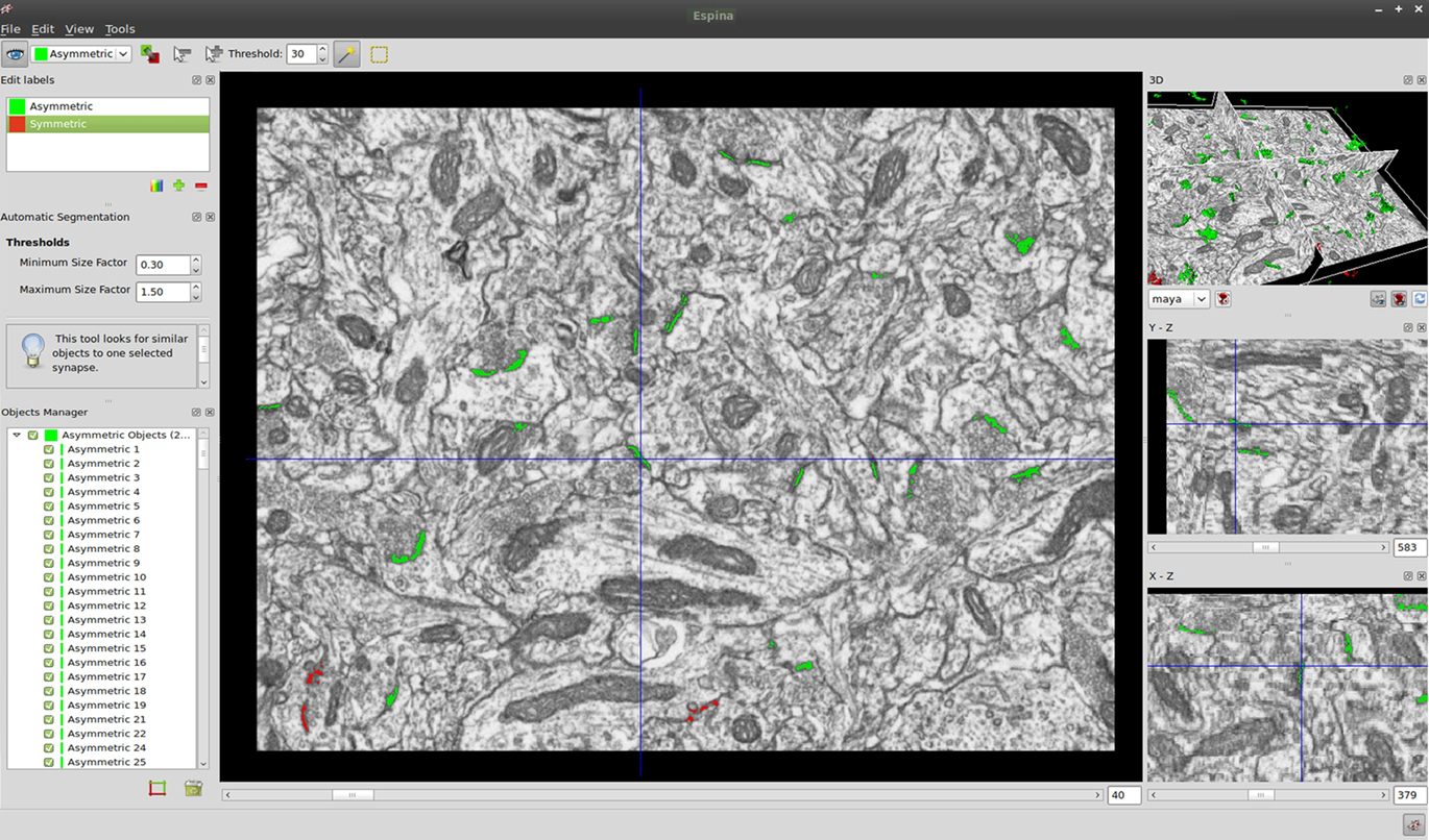
Figure 2. Screenshot of the user interface showing the main window and the three additional auxiliary windows. In the main window the sections are viewed through the x–y plane, as they were obtained by FIB/SEM microscopy. The other two orthogonal planes, y–z and x–z, are also shown in their respective windows. The 3D window shows the three orthogonal planes and the 3D reconstruction of the segmented objects. The location of the mouse pointer is marked by crosshairs in all the windows. Segmented objects appear in green or red according to the colors selected by the user. Each segmented object is given a unique name and number, and it is listed in the “Objects manager” window. Although numerous synaptic junctions are apparently split into two or more parts, these parts are connected in other sections of the series (see also Video 1 in Supplementary Material).

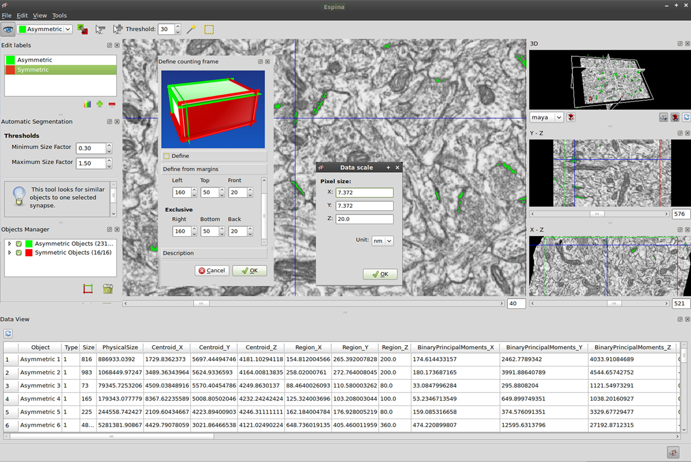
Figure 3. Detail of some controls available to the user. Calibration of the voxel size is applied using the “Data Scale” window, where the values for the x, y, and z axes must be entered independently. Using the “Define counting frame” window the user can choose the position of the six planes. By default, when viewed in the main window, the acceptance planes (in green) correspond to the front, top and left sides of the stack while the exclusion planes (in red) are the back, right, and bottom sides. The “Data viewer” window shows different geometrical values extracted from the reconstructed 3D objects (see text for details).

3D Navigation within the Stack

The user can navigate within the image stack using the sliders located at the bottom of the window or by selecting the desired window and using the mouse wheel. When the mouse is situated at any position in a window, its location can be marked by crosshairs in all the windows by pressing control-left click. This greatly facilitates the identification of dubious synapses or other structures since the three orthogonal sections of any object can be viewed simultaneously, and the position of these sections can be modified interactively by the user. The 3D window represents the three orthogonal planes, crossing at the point marked by the mouse (Figures 2 and 4). Sections and reconstructed objects can be shown or hidden to facilitate navigation. One of two display modes can be chosen: the first shows a 3D volume reconstruction of the objects that is automatically refreshed when an object is added or deleted; the second shows an accurate 3D volume reconstruction of the objects that, for efficiency, must be refreshed by clicking on the “Refresh” button.

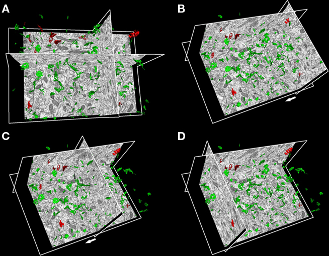
Figure 4. (A) 3D reconstruction of the segmented synaptic junctions in a stack. (B–D) The user can modify the position of any plane to visualize the 3D reconstructed objects. In this example, one plane has been displaced (following the direction of the arrow) to show different views. Green objects represent asymmetric synaptic profiles and red objects symmetric synaptic profiles.

Spatial Calibration

By default, cubic voxels of 1 cubic pixel are used. However, in practice voxels will rarely be cubic since the resolution in the x–y plane is usually better than the thickness of the section. For example, we currently use image pixel sizes that typically range between 3 and 10 nm per pixel in the x and y axes, although the sections are 20 nm thick in the z axis. Thus, the voxel size must be entered independently in the x, y, and z axes. Once this is done, all measurements and calculations will be based on this spatial calibration and the data will be expressed in the units chosen by the user (Figure 3). The 3D rendering of the stack and reconstructed objects will also be scaled to the calibrated voxel size.

The Unbiased Counting Brick

In order to quantify the number of objects per unit volume, a 3D counting frame must be constructed within the stack. This unbiased counting brick is a regular rectangular prism bounded by three acceptance planes and three exclusion planes (Howard and Reed, 2005; Figure 3). All objects within the counting brick or intersecting any of the acceptance planes will be counted, while any object outside the counting brick or intersecting any of the exclusion planes will not. The user can choose the position of the six planes. By default, when viewed in the main window, the acceptance planes correspond to the front, top, and left sides of the stack, while the exclusion planes are the back, right, and bottom sides. The margins between the counting brick and the borders of the stacks must be set carefully, especially for the acceptance planes. These margins can be chosen by entering the desired distances for the top, bottom, left, and right planes. For the front and back planes, the user can choose a section near the beginning of the series and another near the end of the series as the acceptance and exclusion planes.

Segmentation of Synaptic Junctions

Manual Synaptic Junction Segmentation

There are two different means to perform synaptic junction segmentation. In the first of these the synaptic junctions must be identified by the user and selected manually. The user must click on the “Add synapse” tool and then click on any synaptic junction that appears in the main panel, or in any of the other two orthogonal planes (Figure 2). The synapse is extracted using heuristics based on two features: gray levels and connectivity. The seed value clicked by the user, combined with a gray threshold value, allows the 3D propagation of the seed around the neighboring voxels following a region growing scheme with six- connectivity: those voxels that fit into the interval [seed − gray_threshold, seed + gray_threshold] are assigned to the label that identifies the new synapse. This criteria is applied reiteratively over the new voxels aggregated until there are no more voxels with values inside the gray level interval defined. The gray level threshold can be adjusted between 0 and 255 until satisfactory results are obtained, although the features that synapses usually present permit a rapid identification with very little user intervention. For example, a synaptic junction appearing in six consecutive sections, would typically take several minutes to be manually contoured by the user, whereas the same procedure will take only a few seconds with our software. A unique identification number is automatically assigned to each segmented object, which will serve as a key label for object management (Figures 2 and 3). At any moment, the user may also edit the color and name of the resulting segmented object. The result of segmentation is the 3D reconstruction of the objects (Figure 4 and Video 1 in Supplementary Material). All the voxels comprising a segmented synaptic junction are connected and they are considered as a single object, even though in individual 2D sections it may appear that a given junction is split into two or several parts. The representation of objects can be saved in standard STL format.

Magic Wand Segmentation of Synaptic Junctions

This second method of segmentation permits the automatic segmentation of multiple synaptic junctions. It requires that one or several synaptic junctions have been segmented manually. Once the magic wand tool is selected, the user must select one of the previously segmented synaptic junctions to act as a reference. Next, the application will automatically search for similar objects within the stack, in terms of gray level and size, and all of them will be segmented (Figure 2). Similar heuristics to those described in the manual operation are applied to magic wand segmentation. This is a computationally demanding process and multiple threads are launched to segment several objects in parallel. Several seeds are sequentially defined following a deterministic process to avoid duplicating computations. The search for new candidates is pruned by matching the gray level and size parameters of the reference synaptic junction to the data extracted from subsequent candidates. The first step is to binarize the stack of images looking for the voxels whose gray level is within the range defined by the voxels of the reference object. The second step consists of pruning all the candidates (connected pixels) in order to select those that fit into the size range. If the result is not satisfactory, the user may repeat the automatic segmentation process, again adjusting the thresholds as in the manual operation. In addition, incorrectly extracted objects can be manually discarded by selecting the delete control and simply clicking on the erroneous objects with the mouse.

The 3D Region of Interest

The same operations described above can be performed within a 3D region of interest (ROI; Figure 5). This ROI can be selected with the ROI button to set its height and width in the x–y plane, and with two other buttons that establish the depth dimension by selecting sections that define the front and back limits. Once the ROI has been selected, it can be magnified and translated independently of the rest of the stack. This is especially useful when the gray level of the object to be segmented is similar to the surrounding structures, and automatic segmentation tends to spread outside the synaptic junction. This is particularly the case of many symmetric synapses as their post-synaptic densities are much less pronounced than those of asymmetric synapses and thus, the synaptic junction only differs slightly from the adjacent non-synaptic membranes.

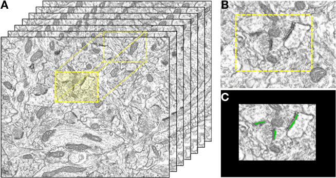
Figure 5. (A) A region of interest (ROI) can be defined in 3D. In this example, a ROI (in yellow) has been chosen to delimit the working area. The ROI can be magnified and translated independently of the rest of the stack. (B) Higher magnification of the ROI. (C) Segmentation of three asymmetric synapses (in green) inside the ROI.

The Object Manager

Segmented objects can be easily managed using a specific widget that allows the list of objects to be manipulated graphically (Figures 2 and 3). Objects can be grouped in categories, allowing the data to be better organized. Each object can be individually selected/unselected to show/hide each separate object. Objects can be removed one by one from the list by just clicking on them and then selecting the delete control. The object manager is not only coupled to the segmentation widgets but also to the unbiased counting brick. Therefore, changes in the limits of the counting brick include or exclude objects accordingly after selecting the counting brick control.

The Data Viewer

The final step of the working session is the extraction of the geometrical measurements for each object segmented. This widget groups the information presented by object classes, allowing the easy and direct comparison of features between several instances of the same class (Figure 3). We have defined the features on which the analysis of synaptic junction morphology is focused, although new parameters can be easily incorporated if new requirements are necessary. The data viewer shows the following attributes:

o Object label and category assigned.

o Size of the object, defined as the number of voxels.

o Physical size, defined as the real object size after multiplying the size by the voxel size.

o Center of gravity of the object, measured in physical units.

o Physical dimension of the bounding box.

o Binary principal moments obtained over the physical units.

o Principal axes of the object.

o Feret diameter, defined as the value of the minimum sphere diameter that circumscribes the object measured in physical units.

o Physical size of the equivalent ellipsoid, obtained from the principal axes of the object.

o Number of synaptic junctions, symmetric or asymmetric, per unit volume.

All these measurements can be easily exported to the standard CSV spreadsheet format. The dimensions of the counting brick are also saved along with the parameters collected in the data viewer widget in order to have a reference of the analysis performed.

Technologies Used in the Implementation

The scrum development methodology was followed as it fits very well to the time requirements established to implement the tool and the environment found in our case (Rising and Janoff, 2000). This methodology favors quick software development based on small sprints, each one producing a new improvement on the tool. The following basic milestones were defined in the early stages of development: tuning of the segmentation algorithm in order to prove the feasibility of the approach selected, implementation of the 3D navigation function to allow users to visualize and move within the stack, and GUI improvement to favor the usability of the tool. Later milestones focused on efficiency issues to achieve the shortest possible response times and new functionalities were gradually added to the tool (e.g., the magic wand, the object manager, the spatial calibration, the unbiased counting brick, the restriction of the segmentation area to the ROI, the data viewer and, in the future, extension of the input/output capabilities to manage other file formats like TIFF images or VRML scenarios). Currently, we have successfully installed the tool on several systems with Linux and Windows, and it is expected that it will also migrate without problems to Mac OS. For this purpose, we have chosen a set of stable and widely tested free distribution tools that make this objective easier to attain: Python vs. 2.6 and C++ as programming languages; ITK vs. 3.16 as the image processing library; VTK vs. 5.4 as the visualization library; and QT for the user interface development. Python allows for rapid development, while C++ ensures code efficiency when needed. ITK and VTK provide a vast collection of classes and functions that implement almost all the algorithms required to date^5,6. The LabelMap class that provides services for object manipulation, labeling and feature extraction has been especially useful (Lehmann, 2008). QT supplies all the widgets and controls that the user needs in a very friendly interface⁷.

Conclusion

ESPINA establishes new strategies to handle and visualize complex images like those obtained through FIB/SEM, improving response times and interactivity, thereby facilitating the analysis of the images. The study of synapses has been improved by accelerating the identification, quantification, and reconstruction of synapses in the large tissue volumes obtained by FIB/SEM. The tool deals satisfactorily with images at different resolutions, opening new opportunities to analyze other structures found in FIB/SEM or other image stacks.

The tool offers definite advantages over other packages that implement tagging or contour tracing for synaptic junction segmentation. In a normal operation, several clicks are sufficient to reconstruct the 3D morphology of the synaptic junction in just a few seconds. In an optimal case, most synapses can be automatically extracted from the stack by the user with a single click, only requiring revision of the false positive and false negative synaptic junctions. Automatic feature extraction is the final step to avoid intensive user manipulation since multiple geometric parameters are calculated from the reconstructed 3D objects. Collected measurements can be easily expanded in future versions if necessary.

ESPINA can be downloaded free as a multiplatform package⁸. One problem to resolve in terms of the tool’s distribution is to merge all the libraries needed in a sufficiently compact size, reducing the excessive disk demand. We think that we can still improve this aspect in future versions. Further improvements may be introduced to resolve the difficulties found in segmenting symmetric synapses. Identification of the vesicles that appear besides the synaptic junction may help to introduce new heuristic parameters that refine the automatic extraction of synapses. We expect that ESPINA will also be useful to analyze other morphological structures found in FIB/SEM or other stacks, like mitochondria, axon and dendrite membranes, microtubules, etc. Also, more work will be needed to expand the input/output capabilities of ESPINA to a wider range of file formats and to other microscopy techniques.

Conflict of Interest Statement

The authors declare that the research was conducted in the absence of any commercial or financial relationships that could be construed as a potential conflict of interest.

Acknowledgments

We thank A. I. García, I. Fernaud, and L. Valdés for their technical assistance. This work was supported by grants from the following entities: Centre for Networked Biomedical Research into Neurodegenerative Diseases (CIBERNED, CB06/05/0066) and the Spanish Ministry of Education, Science and Innovation (grants BFU2006-13395; SAF2009-09394 to Javier DeFelipe; TIN2010-21289 and the Cajal Blue Brain Project).

Supplementary Material

The Video 1 for this article can be found online at http://www.frontiersin.org/neuroscience/neuroanatomy/paper/10.3389/fnana.2011.00018/

Video 1. Shows a working session of ESPINA and demonstrates some of its features and capabilities. Please consider that some image quality has been lost during the video compression process.

Footnotes

References

Anderson, J. R., Jones, B. W., Yang, J., Shaw, M. V., Watt, C. B., Koshevoy, P., Spaltenstein, J., Jurrus, E., Kannan, U. V., Whitaker, R. T., Mastronarde, D., Tasdizen, T., and Marc, R. E. (2009). A computational framework for ultrastructural mapping of neural circuitry. PLoS Biol. 7, e1000074. doi: 10.1371/journal.pbio.1000074
Arellano, J. I., Benavides-Piccione, R., Defelipe, J., and Yuste, R. (2007). Ultrastructure of dendritic spines: correlation between synaptic and spine morphologies. Front. Neurosci. 1:131–143. doi: 10.3389/neuro.01/1.1.010.2007
Colonnier, M. (1968). Synaptic patterns on different cell types in the different laminae of the cat visual cortex. An electron microscope study. Brain Res. 9, 268–287.
Colonnier, M., and Beaulieu, C. (1985). An empirical assessment of stereological formulae applied to the counting of synaptic disks in the cerebral cortex. J. Comp. Neurol. 231, 175–179.
DeFelipe, J., Alonso-Nanclares, L., and Arellano, J. I. (2002). Microstructure of the neocortex: comparative aspects. J. Neurocytol. 31, 299–316.
DeFelipe, J., Marco, P., Busturia, I., and Merchán-Pérez, A. (1999). Estimation of the number of synapses in the cerebral cortex: methodological considerations. Cereb. Cortex 9, 722–732.
Denk, W., and Horstmann, H. (2004). Serial block-face scanning electron microscopy to reconstruct three-dimensional tissue nanostructure. PLoS Biol. 2, e329. doi: 10.1371/journal.pbio.0020329
Fiala, J. C. (2005). Reconstruct: a free editor for serial section microscopy. J. Microsc. 218, 52–61.
Fuchs, R., and Hauser, H. (2009). Visualization of multi-variate scientific data. Comput. Graph. Forum 28, 1670–1690.
Gray, E. G. (1959). Axo-somatic and axo-dendritic synapses of the cerebral cortex: an electron microscope study. J. Anat. 93, 420–433.
Harris, K. M., Perry, E., Bourne, J., Feinberg, M., Ostroff, L., and Hurlburt, J. (2006). Uniform serial sectioning for transmission electron microscopy. J. Neurosci. 26, 12101–12103.
Hoffpauir, B. K., Pope, B. A., and Spirou, G. A. (2007). Serial sectioning and electron microscopy of large tissue volumes for 3D analysis and reconstruction: a case study of the calyx of held. Nat. Protoc. 2, 9–22.
Houser, C. R., Vaughn, J. E., Hendry, S. H. C., Jones, E. G., and Peters, A. (1984). “GABA neurons in the cerebral cortex,” in Cerebral Cortex, Vol. 2, Functional Properties of Cortical Cells, eds E. G. Jones and A. Peters (New York: Plenum Press), 63–89.
Howard, C. V., and Reed, M. G. (2005). Unbiased Stereology: Three-Dimensional Measurement in Microscopy, 2nd Edn. Oxon: Garland Science/BIOS Scientific Publishers.
Jeong, W. K., Beyer, J., Hadwiger, M., Blue, R., Law, C., Vazquez, A., Reid, C., Lichtman, J., and Pfister, H. (2010). SSECRETT and NeuroTrace: interactive visualization and analysis tools for large-scale neuroscience datasets. IEEE Comput. Graph. 30, 58–70.
Knott, G., Marchman, H., Wall, D., and Lich, B. (2008). Serial section scanning electron microscopy of adult brain tissue using focused ion beam milling. J. Neurosci. 28, 2959–2964.
Kremer, J. R., Mastronarde, D. N., and McIntosh, J. R. (1996). Computer visualization of three-dimensional image data using IMOD. J. Struct. Biol. 116, 71–76.
Merchán-Pérez, A., Rodriguez, J., Alonso-Nanclares, L., Schertel, A., and Defelipe, J. (2009a). Counting synapses using FIB/SEM microscopy: a true revolution for ultrastructural volume reconstruction. Front. Neuroanat. 3:18. doi: 10.3389/neuro.05.018.2009
Merchán-Pérez, A., Rodriguez, J., Ribak, C. E., and DeFelipe, J. (2009b). Proximity of excitatory and inhibitory axon terminals adjacent to pyramidal cell bodies provides a putative basis for nonsynaptic interactions. Proc. Natl. Acad. Sci. U.S.A. 106, 9878–9883.
Peters, A., Palay, S. L., and Webster, H. D. (1991). The Fine Structure of the Nervous System: Neurons and their Supporting Cells, 3rd Edn. New York: Oxford University Press.
Pruggnaller, S., Mayr, M., and Frangakis, A. S. (2008). A visualization and segmentation toolbox for electron microscopy. J. Struct. Biol. 164, 161–165.
Rising, L., and Janoff, N. S. (2000). The SCRUM software development process for small teams. IEEE Softw. 17, 26–32.
Keywords: synapses, segmentation, 3D reconstruction, quantification, software, focused ion beam, scanning electron microscopy
Citation: Morales J, Alonso-Nanclares L, Rodríguez J-R, DeFelipe J, Rodríguez Á and Merchán-Pérez Á (2011) ESPINA: a tool for the automated segmentation and counting of synapses in large stacks of electron microscopy images. Front. Neuroanat. 5:18. doi: 10.3389/fnana.2011.00018
Received: 05 November 2010;
Paper pending published: 01 February 2011;
Accepted: 01 March 2011;
Published online: 18 March 2011.
Edited by:
Idan Segev, The Hebrew University of Jerusalem, IsraelReviewed by:
Jose L. Lanciego, University of Navarra, SpainEdward L. White, Ben-Gurion University, Israel
Yoshiyuki Kubota, National Institute for Physiological Sciences, Japan
Copyright: © 2011 Morales, Alonso-Nanclares, Rodríguez, DeFelipe, Rodríguez and Merchán-Pérez. This is an open-access article subject to an exclusive license agreement between the authors and Frontiers Media SA, which permits unrestricted use, distribution, and reproduction in any medium, provided the original authors and source are credited.
*Correspondence: Ángel Merchán-Pérez, Laboratorio de Circuitos Corticales, Centro de Tecnología Biomédica, Universidad Politécnica de Madrid, Campus Montegancedo S/N, Pozuelo de Alarcón, 28223 Madrid, Spain. e-mail: amerchan@fi.upm.es