1
Frankfurt Institute of Advanced Studies, Johann Wolfgang Goethe University, Frankfurt am Main, Germany
2
Department of Neurophysiology, Max Planck Institute for Brain Research, Frankfurt am Main, Germany
Understanding the dynamics of recurrent neural networks is crucial for explaining how the brain processes information. In the neocortex, a range of different plasticity mechanisms are shaping recurrent networks into effective information processing circuits that learn appropriate representations for time-varying sensory stimuli. However, it has been difficult to mimic these abilities in artificial neural network models. Here we introduce SORN, a self-organizing recurrent network. It combines three distinct forms of local plasticity to learn spatio-temporal patterns in its input while maintaining its dynamics in a healthy regime suitable for learning. The SORN learns to encode information in the form of trajectories through its high-dimensional state space reminiscent of recent biological findings on cortical coding. All three forms of plasticity are shown to be essential for the network’s success.
The mammalian neocortex is the seat of our highest cognitive functions. Despite much effort, a detailed characterization of its complex neural dynamics and an understanding of the relationship between these dynamics and cognitive processes remain elusive. Cortical networks present an astonishing ability to learn and adapt via a number of plasticity mechanisms which affect both their synaptic and neuronal properties. These mechanisms allow the recurrent networks in the cortex to learn representations of complex spatio-temporal stimuli. Interestingly, neuronal responses are highly dynamic in time (even when the stimulus is static) (Broome et al., 2006
) and contain a rich amount of information about past events (Brosch and Schreiner, 2000
; Bartlett and Wang, 2005
; Broome et al., 2006
; Nikolic et al., 2006
).
But mimicking these features in artificial neural networks has proven to be very difficult. The first models that could address temporal tasks have incorporated in their structure an explicit representation of time (Elman and Zipser, 1988
). Recurrent neural networks (RNNs) were the first models to represent time implicitly, through the effect that is has on processing (Hopfield, 1982
; Elman, 1990
). In the recently developed framework of ‘reservoir’ computing (Jaeger, 2001
; Maass et al., 2002
), a randomly structured RNN non-linearly transforms a time varying input signal into a spatial representation. At each time step, the network combines the incoming stimuli with a volley of recurrent signals containing a memory trace of recent inputs. For a network with N neurons, the resulting activation vector at a discrete time t, can be regarded as a point in a N-dimensional space. Over time, these points form a pathway through the state space also referred to as a neural trajectory. A separate read-out layer is trained, with supervised learning techniques, to map different parts of the state space to desired outputs. In real cortical networks, experimental evidence has shown that different stimuli elicit different trajectories while for a given stimuli the activity patterns evolve in time in a reproducible manner (Broome et al., 2006
; Churchland et al., 2007
). Furthermore, identical trials can present a high response variability, but the resulting trajectories are not dominated by noise (Mazor and Laurent, 2005
; Broome et al., 2006
; Churchland et al., 2007
). Reservoir networks do not require classical attractor states and are compatible with the view that cortical computation is based on transient dynamics (Mazor and Laurent, 2005
; Durstewitz and Deco, 2008
; Rabinovich et al., 2008
). It has been shown that neural systems may exhibit transients of long durations which carry more information about the stimulus then the steady states towards which the activity evolves (Mazor and Laurent, 2005
).
Attempts to endow RNNs with unsupervised learning abilities by incorporating biologically plausible local plasticity mechanisms such as spike-timing-dependent plasticity (STDP) (Markram et al., 1997
; Bi and Poo, 1998
) have remained largely unsuccessful (and often unpublished). The problem is most difficult, because structural changes induced by plasticity will impact the network’s dynamics giving rise to altered firing patterns between neurons. These altered firing patterns can further induce changes in connectivity through the plasticity mechanisms and so forth. Understanding and controlling the ensuing self-organization of network structure and dynamics as a function of the network’s inputs is a formidable challenge.
The key to the brain’s solution to this problem may be the synergistic combination of multiple forms of neuronal plasticity. There has been extensive evidence that synaptic learning is accompanied by homeostatic mechanisms. Synaptic scaling regulates the total synaptic drive received by a neuron but maintains the relative strength of synapses established during learning (Turrigiano et al., 1998
). At the same time, intrinsic plasticity (IP) was shown to directly regulate neuronal excitability (Desai et al., 1999
; Zhang and Linden, 2003
). In a RNN, IP induced robust homeostatic effects on the network dynamics (Steil, 2007
; Schrauwen et al., 2008
). But there is only little work combining several forms of plasticity in RNNs (Lazar et al., 2007
).
In the following, we present a RNN of threshold units combining three different forms of plasticity that learns to efficiently represent and “understand” the spatio-temporal patterns in its input. The SORN model (self-organizing recurrent network) consists of a population of excitatory cells and a smaller population of inhibitory cells (Figure 1
). The connectivity among excitatory units is sparse and subject to a simple STDP rule. Additionally, synaptic normalization (SN) keeps the sum of an excitatory neuron’s afferent weights constant, while IP regulates a neuron’s firing threshold to maintain a low average activity level. The network receives input sequences composed of different symbols and learns the structure embedded in these sequences in an unsupervised manner. The three types of plasticity mechanisms induce changes in network dynamics which we assess via hierarchical clustering and principal component analysis (PCA). In addition, we train a separate readout layer with supervised learning techniques and compare the performance of our network with that of fixed random networks constructed in the spirit of reservoir computing.
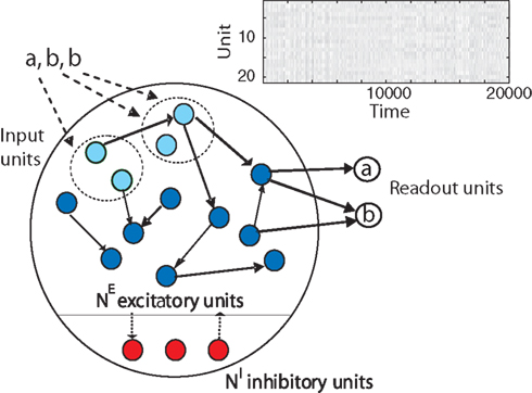
Figure 1. The self-organizing recurrent neural network (SORN) comprises populations of excitatory (blue) and inhibitory (red) cells. Directed connections with variable strength between neurons are indicated by black arrows. Some of the excitatory cells also receive external input (light blue). Three forms of plasticity interact to shape the dynamics of the network keeping them in a healthy regime and allowing the network to discover structure in its inputs. A population of readout units is trained with supervised learning methods.
We show that only the combination of all three types of plasticity allows the network to (a) learn to effectively represent the spatio-temporal structure of its inputs, (b) maintain ‘healthy’ dynamics
1
that make efficient use of all the network’s resources, and (c) perform much better on prediction tasks compared to random networks without plasticity. Furthermore, the network dynamics are consistent with a range of neurophysiological findings.
The Sorn Model
Network definition
We consider a network with NE excitatory (E) and NI = 0.2 × NE inhibitory (I) threshold units. Neurons are coupled through weighted synaptic connections, where Wij is the connection strength from unit j to unit i, with i ≠ j. All possible connections between the excitatory and inhibitory neuron populations are present (WIE and WEI), while the excitatory–excitatory connections (WEE) are sparse and random with a mean number λW of incoming and outgoing connections per neuron. Direct connections between inhibitory units are not present. The weight strengths are drawn from the interval [0, 1] and subsequently normalized such that the incoming connections to a neuron sum up to a constant value:  ,
,  and
and  . Inputs are time series U(t) of different symbols (letters or digits). Each symbol is associated with a specific group of NU input units which all receive a positive input drive (νU = 1) when that particular symbol is active.
, and . Inputs are time series U(t) of different symbols (letters or digits). Each symbol is associated with a specific group of NU input units which all receive a positive input drive (νU = 1) when that particular symbol is active.The network state, at a discrete time t, is given by the binary vectors  and
and  corresponding to the activity of the excitatory and inhibitory units, respectively. The evolution of the network state is described by:
and corresponding to the activity of the excitatory and inhibitory units, respectively. The evolution of the network state is described by:
The TE and TI are threshold values for the excitatory and inhibitory units. They are initially drawn from a uniform distribution in the interval  and
and  , respectively. The heaviside step function Θ(.) constrains the activation of the network at time t to a binary representation: a neuron fires if the total drive it receives is greater then its threshold, otherwise it stays silent.
and , respectively. The heaviside step function Θ(.) constrains the activation of the network at time t to a binary representation: a neuron fires if the total drive it receives is greater then its threshold, otherwise it stays silent.At each time step the activity of the network is determined both by the inputs  and the propagation of the previously emitted spikes through the network. This recurrent drive received by unit i is given by:
and the propagation of the previously emitted spikes through the network. This recurrent drive received by unit i is given by:
Based on this, we define a “pseudo state” x′(t) that only depends on the recurrent drive:

This equation is identical to Eq. 1, but lacking the input drive  . Most of our analysis focuses on the pseudo states x′(t) as the network’s internal representation of previous inputs, although it may contain less information than R(t) due to the thresholding operation.
. Most of our analysis focuses on the pseudo states x′(t) as the network’s internal representation of previous inputs, although it may contain less information than R(t) due to the thresholding operation.Plasticity mechanisms
The network relies on three forms of plasticity: STDP, synaptic scaling of the excitatory–excitatory connections, and IP regulating the thresholds of excitatory units.
Learning with STDP is constrained to the set of WEE synapses. We use a simple model of STDP that strengthens the synaptic weight  by a fixed amount ηSTDP = 0.001 whenever unit i is active in the time step following activation of unit j. When unit i is active in the time step preceding activation of unit j,
  is weakened by the same amount:
by a fixed amount ηSTDP = 0.001 whenever unit i is active in the time step following activation of unit j. When unit i is active in the time step preceding activation of unit j, is weakened by the same amount:
STDP changes the synaptic strength in a temporally asymmetric “causal” fashion. The changes introduced by STDP can push the activity of the network to grow or shrink in an uncontrolled manner. To keep the activity balanced during learning we make use of additional homeostatic mechanisms that are sensitive to the total level of synaptic efficacy and the post-synaptic firing rate.
SN proportionally adjusts the values of incoming connections to a neuron so that they sum up to a constant value. Specifically, the WEE connections are rescaled at every time step according to:

This rule does not change the relative strengths of synapses established by STDP but regulates the total incoming drive a neuron receives.
An IP rule spreads the activity evenly across units, such that on average each excitatory neuron will fire with the same target rate HIP. To this end, a unit that has just been active increases its threshold while an inactive unit lowers its threshold by a small amount:

where ηIP = 0.001 is a small learning rate. We set the target rate to HIP = 2 × NU/NE in which the input spikes are approximately half of the total number of spikes. Other settings of HIP do not necessarily lead to the desired improvements in prediction performance (see Appendix).
The implementation of the model described above and the simulations presented in Section “Results” were performed in Matlab.
SORNs Outperform Static Reservoirs
We demonstrate the SORN’s ability to learn spatio-temporal structure in its inputs with a “counting” task, especially designed to test the memory property of the reservoir. To this end, we construct input sequences U(t) as random alternations of two “words” ‘abbb…bc’ and ‘eddd…df’, composed of n + 2 “letters”, with letters ‘b’ and ‘d’ repeating n times. In order to predict the next input letter correctly, the network has to learn to “count” how many repetitions of letters ‘b’ and ‘d’ it has already seen. Increasing n raises the difficulty of the task. We compare SORNs with all three forms of plasticity to static networks without plasticity. Networks of different sizes NE have their initial parameters set to NU = 5% × NE,  ,
,  and λW = 10. For small static reservoirs, the parameters are tuned such that their dynamics is critical and the networks’ firing rate is similar to the rate exhibited by SORNs structured by plasticity (see Supplementary Material and Section “Occluder Task”). It has been argued that a tuning of network dynamics to criticality should bring the performance of static reservoir networks close to the optimal performance (Bertschinger and Natschläger, 2004
). To compute prediction performance, 5000 steps of network activity are simulated and a readout is trained in a supervised fashion to predict the next input [U(t)], e.g., ‘a’, or ‘c’, or 5th repetition of ‘b’, etc., based on the network’s internal state [x′(t)] after presentation of the preceding letter [U(t − 1)]. We use the Moore–Penrose pseudoinverse method that minimizes the squared difference between the output of the readout neurons and the target output value. The quality of the readout (the network performance) is assessed on a second sample of 5000 steps of activity using an independent input sequence.
and λW = 10. For small static reservoirs, the parameters are tuned such that their dynamics is critical and the networks’ firing rate is similar to the rate exhibited by SORNs structured by plasticity (see Supplementary Material and Section “Occluder Task”). It has been argued that a tuning of network dynamics to criticality should bring the performance of static reservoir networks close to the optimal performance (Bertschinger and Natschläger, 2004
). To compute prediction performance, 5000 steps of network activity are simulated and a readout is trained in a supervised fashion to predict the next input [U(t)], e.g., ‘a’, or ‘c’, or 5th repetition of ‘b’, etc., based on the network’s internal state [x′(t)] after presentation of the preceding letter [U(t − 1)]. We use the Moore–Penrose pseudoinverse method that minimizes the squared difference between the output of the readout neurons and the target output value. The quality of the readout (the network performance) is assessed on a second sample of 5000 steps of activity using an independent input sequence.
, and λW = 10. For small static reservoirs, the parameters are tuned such that their dynamics is critical and the networks’ firing rate is similar to the rate exhibited by SORNs structured by plasticity (see Supplementary Material and Section “Occluder Task”). It has been argued that a tuning of network dynamics to criticality should bring the performance of static reservoir networks close to the optimal performance (Bertschinger and Natschläger, 2004
). To compute prediction performance, 5000 steps of network activity are simulated and a readout is trained in a supervised fashion to predict the next input [U(t)], e.g., ‘a’, or ‘c’, or 5th repetition of ‘b’, etc., based on the network’s internal state [x′(t)] after presentation of the preceding letter [U(t − 1)]. We use the Moore–Penrose pseudoinverse method that minimizes the squared difference between the output of the readout neurons and the target output value. The quality of the readout (the network performance) is assessed on a second sample of 5000 steps of activity using an independent input sequence.The SORNs are exposed to the input sequences for 50,000 time steps. Then, all their weights and thresholds are frozen and a readout is trained in the same manner.
Since the input sequences are partly random – the order of letters within a word is fixed but the order of words is random – prediction performance is inherently limited. We define a normalized performance measure that obtains a score of 1 when the network always correctly predicts the next letter and its position within a word but is at chance level for guessing the first letter of the next word (either ‘a’ or ‘e’). Figure 2
compares the performance of SORNs and static reservoir networks. For any given network size (NE) and any given task difficulty (n), the plastic SORNs perform considerably better than their randomly structured counterparts (Figure 2
A). For the same task difficulty n, larger networks perform better then smaller networks. For a given network size the SORNs achieve a performance greater than 0.95 for much higher values of n compared to the static reservoirs (Figure 2
B). A more detailed analysis of the network performance as a function of various initial parameter settings is given in the Appendix.
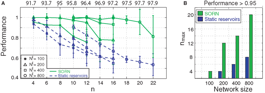
Figure 2. (A) Average normalized performance of 10 plastic SORNs and 10 static reservoir networks of size NE, for different values of n. Numbers on top indicate optimal absolute performance achievable in the task. Error bars indicate standard deviation. (B) We show nmax, the highest value of n where normalized performance exceeds 95%, as a function of network size. Plastic networks succeed for substantially harder problems compared to random reservoirs.
SORNs Learn Effective Internal Representations
To better understand the reason underlying the performance advantage of SORNs over static reservoirs, we performed hierarchical clustering and PCA on the networks’ internal representations.
We performed agglomerative hierarchical clustering of the networks’ internal state representations (x′). Each pattern of activity x′(t) is a point in a NE-dimensional space. Agglomerative clustering starts by considering each of these points as centers of their own cluster. The distance between two clusters is computed as the Euclidean distance between their centers. Repeatedly, the two closest clusters are merged into a single cluster, until the entire data are collapsed.
In Figures 3
A,E we present a snapshot of the last 20 clusters of agglomerative clustering, for an example network with NE = 200, NU = 10,  ,
,  , λ = 10 during a counting task with n = 8. In the case of randomly structured reservoir networks, the cluster structure of internal representations only weakly reflects the underlying input conditions (Figure 3
A). Many of the emerging clusters combine network states resulting from distinct input conditions, i.e., the networks internal representation easily confuses, say, the 5th repetition of letter ‘b’ with its 6th repetition. In fact most clusters lump together as many as seven input conditions (Figure 3
B). In contrast after 50,000 steps of plasticity, the SORN learns an internal representation that tends to map different input conditions on to distinct network states falling into separate clusters (Figure 3
E). Here, each cluster will combine at most two different input conditions (Figure 3
F). For a parallel with the performance tests from the previous section, the analysis was performed on 5000 steps of activity with frozen weights and thresholds but the network presents similar clustering properties in the presence of plasticity.
, λ = 10 during a counting task with n = 8. In the case of randomly structured reservoir networks, the cluster structure of internal representations only weakly reflects the underlying input conditions (Figure 3
A). Many of the emerging clusters combine network states resulting from distinct input conditions, i.e., the networks internal representation easily confuses, say, the 5th repetition of letter ‘b’ with its 6th repetition. In fact most clusters lump together as many as seven input conditions (Figure 3
B). In contrast after 50,000 steps of plasticity, the SORN learns an internal representation that tends to map different input conditions on to distinct network states falling into separate clusters (Figure 3
E). Here, each cluster will combine at most two different input conditions (Figure 3
F). For a parallel with the performance tests from the previous section, the analysis was performed on 5000 steps of activity with frozen weights and thresholds but the network presents similar clustering properties in the presence of plasticity.
, , λ = 10 during a counting task with n = 8. In the case of randomly structured reservoir networks, the cluster structure of internal representations only weakly reflects the underlying input conditions (Figure 3
A). Many of the emerging clusters combine network states resulting from distinct input conditions, i.e., the networks internal representation easily confuses, say, the 5th repetition of letter ‘b’ with its 6th repetition. In fact most clusters lump together as many as seven input conditions (Figure 3
B). In contrast after 50,000 steps of plasticity, the SORN learns an internal representation that tends to map different input conditions on to distinct network states falling into separate clusters (Figure 3
E). Here, each cluster will combine at most two different input conditions (Figure 3
F). For a parallel with the performance tests from the previous section, the analysis was performed on 5000 steps of activity with frozen weights and thresholds but the network presents similar clustering properties in the presence of plasticity.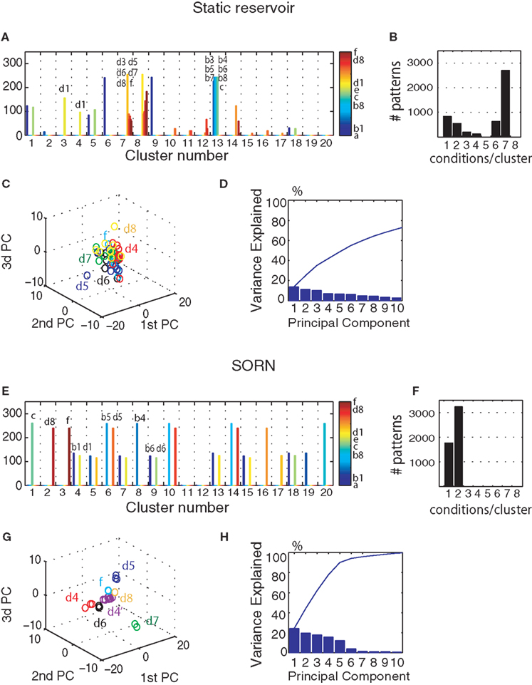
Figure 3. (A) Result of hierarchical clustering of the internal representation of a static random reservoir. Only a single stage with 20 clusters is shown. For each of the 20 clusters, a histogram depicts the different input conditions that contributed to the cluster. Clusters tend to mix many distinct input conditions, especially different repetitions of ‘b’ or ‘d’, instead of keeping them separate. (B) Histogram showing how many different input conditions contribute to each of the 20 clusters. (C) Result of PCA on the pseudo state x′ corresponding to the last six letters of the input sequence ‘eddddddddf’ which we refer to as ‘d4’, ‘d5’, ‘d6’, ‘d7’,‘d8’ and ‘f’. Identical input conditions are spread far apart and strongly overlap with other input conditions. (D) The amount of variance explained by the first principal components. (E–H) Same as (A–D) but for SORNs. (E) The cluster structure in SORNs reflects the different input conditions. (F) Representations of different inputs are comparatively distinct such that only one or two input conditions contribute to each cluster. (G) In PCA space, the different input conditions form compact clusters that are well separated for different input conditions. (H) Most of the variance is captured by only the first few principal components, suggesting more orderly dynamics in the SORNs.
We also performed PCA on the internal network states. In the case of random networks a single input condition produces a cloud of network states that is substantially overlapping with those from other input states within the projection space of the first three PCs (Figure 3
C). In contrast, the SORN develops an internal representation where an input conditions produces a tight cluster of network states that is well separated from those of other input conditions (Figure 3
G). In particular, it learns to internally distinguish different states that have a very similar history of inputs, say, five vs. six repetitions of letter ‘b’. This leads to more orderly and stereotyped trajectories through the network state space in the case of SORNs. This is in line with the greater amount of variance explained by the first few PCs in the SORNs compared to random networks (compare Figures 3
D,H).
Interestingly, as long as plasticity is switched on, the internal representation will keep changing, i.e., the network does not converge. The internal representations of different input conditions tend to change gradually with time. For example, in Figure 3
G the input condition d4 is shown after an additional 5000 time steps of plasticity, as d4’. To function properly, the network requires re-training of the readout as soon as the network’s internal representations change significantly.
Occluder Task
We demonstrate the ability of the SORN to learn effective representations on a second difficult task. Specifically, we consider an input sequence containing random alternations of the following four “words”: ‘12345678’, ‘87654321’, ‘19999998’, ‘89999991’. If we associate different spatial positions with the numbers 1–8, we can interpret these stimuli as left to right and right to left motion of an object along an axis. The symbol ‘9’ can be interpreted as an occluder that obstructs the sight of the object at locations 2–7. This task is more difficult than the counting task in that several words share start and end letters and the repetitive symbol ‘9’ is common in the last two sequences. The bidirectional quality of this stimuli might impose difficulties for the causal STDP rule. The interference of enforced synaptic pathways could decrease the prediction performance of SORNs. On the other hand, due to synaptic competition STDP might encourage one direction of motion and prune away the other. Our results suggest that both of these effects are avoided and SORNs present prediction advantages over random reservoirs.
We choose a network with NE = 200, NU = 15,  ,
,  , and λW = 10. We run the SORN for 200,000 time steps and take snapshots of weights W and thresholds T at every 1000 steps of self-organization through plasticity. We evaluate each of these networks in terms of prediction performance for the one step prediction task. Similarly to the previous experiment, the performance drastically improves (Figure 4
A) and is close to the theoretical optimum for all the different time intervals of self-organization with plasticity. We also assess the criticality of the network dynamics by performing a perturbation analysis. For every state x(t), we perturb the activation of a randomly chosen excitatory neuron (from active to inactive or from inactive to active) creating an altered state
, and λW = 10. We run the SORN for 200,000 time steps and take snapshots of weights W and thresholds T at every 1000 steps of self-organization through plasticity. We evaluate each of these networks in terms of prediction performance for the one step prediction task. Similarly to the previous experiment, the performance drastically improves (Figure 4
A) and is close to the theoretical optimum for all the different time intervals of self-organization with plasticity. We also assess the criticality of the network dynamics by performing a perturbation analysis. For every state x(t), we perturb the activation of a randomly chosen excitatory neuron (from active to inactive or from inactive to active) creating an altered state  . The Hamming distance between x(t) and its perturbed version
  is 1 [d(t) = 1]. We calculate the successor states of x(t) and
  by applying Eq. 1 and obtain x(t + 1) and
  with the Hamming distance d(t + 1). If the average distance
  the network amplifies perturbations and is in a supercritical regime. If
  the network has self-correcting properties and is in a subcritical dynamical regime. When
  the dynamics is said to be critical. Performing perturbation analysis, we find that the network dynamics changes from a critical regime, in the case of static reservoirs, to a subcritical regime for SORNs (Figure 4
B). Interestingly, in the case of SORNs this corresponds to a higher network performance for prediction.
the dynamics is said to be critical. Performing perturbation analysis, we find that the network dynamics changes from a critical regime, in the case of static reservoirs, to a subcritical regime for SORNs (Figure 4
B). Interestingly, in the case of SORNs this corresponds to a higher network performance for prediction.
, , and λW = 10. We run the SORN for 200,000 time steps and take snapshots of weights W and thresholds T at every 1000 steps of self-organization through plasticity. We evaluate each of these networks in terms of prediction performance for the one step prediction task. Similarly to the previous experiment, the performance drastically improves (Figure 4
A) and is close to the theoretical optimum for all the different time intervals of self-organization with plasticity. We also assess the criticality of the network dynamics by performing a perturbation analysis. For every state x(t), we perturb the activation of a randomly chosen excitatory neuron (from active to inactive or from inactive to active) creating an altered state . The Hamming distance between x(t) and its perturbed version is 1 [d(t) = 1]. We calculate the successor states of x(t) and by applying Eq. 1 and obtain x(t + 1) and with the Hamming distance d(t + 1). If the average distance the network amplifies perturbations and is in a supercritical regime. If the network has self-correcting properties and is in a subcritical dynamical regime. When the dynamics is said to be critical. Performing perturbation analysis, we find that the network dynamics changes from a critical regime, in the case of static reservoirs, to a subcritical regime for SORNs (Figure 4
B). Interestingly, in the case of SORNs this corresponds to a higher network performance for prediction.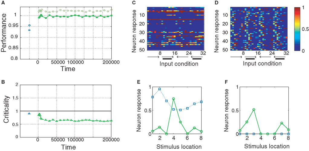
Figure 4. Performance of the SORN and a random reservoir on the “occluder” task. (A) Performance of a readout trained to predict the next input letter. Performance of a static reservoir network (blue symbols left of 0 on the time axis) is worse than that of the SORN. (B) As plasticity unfolds, the dynamics develop from a near-critical regime to a subcritical one. Probability of 50 randomly selected neurons firing for different input conditions in static reservoirs (C) and the SORN (D). In the SORN firing is more specific to particular input conditions. (E,F) Tuning curves for two representative model neurons in a static network (blue squares) and the SORN (green circles). In the SORN, neurons are sparsely active and respond to specific input conditions. In the static networks, some neurons will respond rather unspecifically for all input conditions (E) or not at all (F).
We also compare the tuning of the random reservoir network with the SORN after 50,000 steps of plasticity. For each of these two networks we consider 5000 time steps of network activity (in both cases without plasticity) and count the number of neuron responses corresponding to each of the 32 input conditions: left–right motion (‘12345678’), left–right motion with occluder (‘19999998’), right–left motion (‘87654321’) and right–left motion with occluder (‘89999991’). For the random network we find that a number of neurons are silent and do not fire for any of the input conditions (Figure 4
C). Also the neurons responding to the occluder sequences are not very selective in terms of either location or direction. In contrast, for the SORN all neurons take part in the activity and their responses are input specific (Figure 4
D). We calculated “tuning curves” of two example neurons to illustrate this point in more detail. To this end, we summed the neurons’ responses for each of the eight locations of the visual space irrespective of motion direction or occluder presence. The neuron in (Figure 4
E) responded unselectively to all eight locations before any plasticity (static reservoir case, blue squares) and after learning it has developed a clear preference for location 4 (SORN case, green circles). The neuron in (Figure 4
F) was silent in the initial network setup (static reservoir case). Through plasticity, it developed selectivity for locations 3 and 7 (SORN case). Interestingly, this selectivity is also specific with regard to motion direction. The neuron fires when a stimulus is at location 3 moving to the right, or when the stimulus is at location 7 moving to the left (not shown).
Homeostatic Plasticity Mechanisms are Critical for Maintaining Healthy Dynamics
To better understand the role of the homeostatic plasticity mechanisms accompanying STDP-learning in SORNs, we compare SORNs with plastic reservoirs in which either the synaptic scaling or the IP is switched off. We consider networks receiving unstructured inputs, here in the form of random alternations of six symbols. Thus, there is no specific spatio-temporal structure in the inputs that could be learned during these experiments. The networks (NE = 200, NU = 10,  ,
,  and λW = 10) are shaped in the presence of all three forms of plasticity for 50,000 steps.
, and λW = 10) are shaped in the presence of all three forms of plasticity for 50,000 steps.The results are summarized in Figure 5
. When SN is missing, the network dynamics develop into a regime with seizure-like synchronous bursts of activity (Figure 5
A), even though the network is driven by random inputs. We compared the distribution of the total number of spikes per time step for 10 networks with and without SN (Figure 5
B). In networks with SN the distribution is unimodal and centered at a low activity level. In contrast, networks without SN will show a bimodal distribution such that most units are either active or inactive at the same time. This is also expressed in the average correlation coefficient between neurons. In networks with SN the average correlation coefficient remains close to 0 with an average value of 0.025. For networks that lack SN the average correlation coefficient increases as a function of time to values beyond 0.8 within 50,000 steps of simulation, indicating a high degree of synchronization (Figure 5
C).
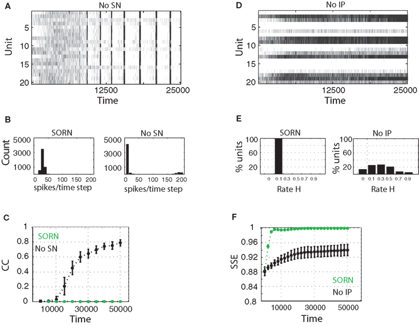
Figure 5. Activity of SORN networks compared to networks missing synaptic normalization (A–C) or intrinsic plasticity (D–F). (A,D) Snapshot of activity for 50 randomly selected reservoir units. (B) Distribution of population activity after 50,000 time steps of simulation. (C) Average correlation coefficient between neurons is dramatically increasing without SN. (E) Distribution of firing rates becomes very wide when IP is missing. (F) Spike source entropy increases to the maximum value for SORN networks, indicating a uniform division of labor across neurons.
When IP is missing a number of neurons remain permanently silent, while others develop an unnaturally high activity (Figure 5
D). We calculated the distribution of average firing rates for 10 such networks. In networks with IP, all excitatory units develop average firing rates close to the desired target rate, which was 0.1 in these experiments. Without IP, the distribution is more spread out with some units staying completely silent and others being active in almost every time step (Figure 5
E). We quantified this effect by following the time evolution of the spike source entropy, which measures how much uncertainty there is about the origin of a spike in the network. It is defined as:
where pi is the probability that a spike is generated by the unit i. SSE achieves its maximum value of 1 if all units fire at the same rate (pi ∝ Hi, where Hi is the firing rate of neuron i). SORNs show an abrupt increase in SSE to a value close to 1, which indicates identical rates across the neuronal population, compared to a smaller value of 0.94 for networks missing IP (Figure 5
F). Due to IP, SORNs make efficient use of all the network’s resources.
Self-organizing recurrent networks are the substrate for neural information processing in the brain. Such networks are shaped by a wealth of plasticity mechanisms which affect synaptic as well as neuronal properties and operate over various time scales (from seconds to days and beyond). Somehow these mechanisms must work together to allow the brain to learn efficient representations for the various tasks it is facing. They shape the neural code and form the foundation on which our higher cognitive abilities are built.
While great progress has been made in characterizing these mechanisms individually, we only have a poor understanding of how they work together at the network level. In a non-linear system like the brain, any local change to, say, a synaptic efficacy potentially alters the pattern of activity at the level of the entire network and may induce further plastic changes to it. To investigate these processes, recent methods for observing the activities of large populations of neurons simultaneously need to be combined with careful measurements of the evolution of their synaptic and intrinsic properties – a formidable task for experimental neuroscience.
Computational modeling and theoretical analysis can contribute to this quest by providing simplified model systems that hopefully capture the essence of some of the brain’s mechanisms and that can reveal underlying principles. In this article, we have introduced the SORN (self-organizing RNN). It combines three different kinds of plasticity and learns to represent and in a way “understand” the structure in its inputs. Maybe its most striking features is the ability to map identical inputs onto different internal representations based on temporal context. For example, it learns to distinguish the 5th repetition of an input from the 6th repetition by finding distinct encodings (internal representations) for the two situations (compare Figure 3
). All this is happening in a completely unsupervised way without any guidance from the outside. The “causal” nature of the STDP rule is at the heart of this mechanism. It allows the network to incorporate predictable input structure into its own dynamics. At the same time, we have shown that STDP needs to be complemented by two homeostatic plasticity mechanisms. Without them the network will lose its favorable learning properties and may even develop seizure-like activity bursts (compare Figure 5
).
Our network can be contrasted to recurrent networks without plasticity. Such static networks have received significant attention in the recent past, giving rise to the field of reservoir computing (Jaeger, 2001
; Maass et al., 2002
). The performance of a reservoir network relies on two requirements: (a) that different inputs to the network result in separable outputs based on the reservoir’s response (the separation property) and that (b) the network activity states maintain information about recent inputs (the fading memory property). Given the high dimensionality of the reservoir, the separation property is easy to meet. Dockendorf et al. (2009)
have confirmed this property for in vitro networks of cortical neurons. The memory property has been addressed in a series of experimental studies, across different brain areas, that compare the neuronal response to a stimulus B vs. the response to B when it was preceded by stimulus A (Brosch and Schreiner, 2000
; Bartlett and Wang, 2005
; Broome et al., 2006
; Nikolic et al., 2006
). For example in (Nikolic et al., 2006
), the authors analyzed neuronal responses in cat primary visual cortex, area 17, to a sequence of two letter images and were able to recover the identity of the first and second letter reliably using a simple linear classifier.
The most important force shaping the representations in the SORN is STDP. Although the STDP model we used is much simplified, it captures what is arguably the essence of STDP: a “causal” modification of synaptic strengths. In recent years much evidence has accumulated suggesting that the brain’s encoding of stimuli is subject to modifications due to STDP-like mechanisms. Several studies showed that repetitive stimulation with temporally patterned inputs causes a rapid STDP-based synaptic reorganization (Yao and Dan, 2001
; Fu et al., 2002
; Yao et al., 2007
). Specifically, in Yao et al. (2007)
a short repeated exposure to natural movies induced a rapid improvement in response reliability in cat visual cortex. Interestingly, the movie stimulation also left a “memory trace” which could be picked up in subsequent spontaneous activity.
It is interesting to note that in all the example tasks we considered the SORNs outperformed optimized versions of recurrent networks without plasticity. We find it unsurprising but rather reassuring that networks that try to discover and incorporate the temporal structure of their inputs into their dynamics outperform static reservoirs. Under repetitive stimulation with temporally structured inputs, SORNs selforganize in efficient ways that boost the network memory and separation properties. In our results, the SORNs could incorporate much longer input sequences as compared to the static reservoirs of similar size (Figure 2
). SORNs developed internal representations where each input condition, reflecting both spatial and temporal aspects of the input, produced a tight cluster of network states that was well separated from those of other input conditions. This results in orderly and stereotyped trajectories through the network state space, that can be easily separated by a linear readout.
Reservoir computing architectures are thought to function best when their dynamics are critical (which we also found true for random reservoirs). It has been proposed that self-organization based on neuronal plasticity is able to achieve critical dynamics (Lazar et al., 2007
; Gómez et al., 2009
). Interestingly, the SORNs develop dynamics that are subcritical (compare Figure 4
). This raises two questions. First, what is the exact mechanism that gives rise to the subcritical dynamics? Second, why are the subcritical dynamics of SORNs superior to the critical dynamics of static networks? Regarding the latter, we speculate that SORNs’ ability to incorporate the predictable sequence of inputs into their internal dynamics makes it unnecessary to maintain criticality, which should give the best fading memory for arbitrary input sequences. But if there is predictable structure in the input, the recurrent network should try to exploit and use it’s resources to model this specific structure rather than striving to have a general purpose fading memory.
The current model is particularly suited for efficient hardware implementation due to the simplicity of the chosen model neurons. In the current design individual neurons do not have any intrinsic memory properties, which makes a strong point that all memory information is maintained by the recurrent dynamics. An open problem is to investigate the generality of these ideas in the context of more elaborate network models based on integrate and fire neurons or conductance based neurons, which also include direct connections between inhibitory units. Future work needs to address if the performance advantage of SORNs over static networks transfers from the simple problems studied here to more difficult engineering problems in time series prediction, speech recognition, etc.
We have shown how the synergistic combination of different local plasticity mechanisms can shape the global structure and dynamics of RNNs in meaningful and adaptive ways. This emergent property could not have been easily predicted on the basis of the individual mechanisms – the whole is more than the sum of its parts. This implies that as we try to understand neural plasticity and how it shapes the brain’s representation and processing, it is insufficient to study individual mechanisms in isolation. Only by studying their interaction at the network level, we have a chance to unravel this mystery.
Performance and Network Settings
For static reservoirs the choice of threshold values for excitatory ( ) and inhibitory units (
 ) plays an important role in determining the network rate H0, defined as the mean fraction of firing neurons per unit of time. Furthermore, the setting of
  and
and  has an impact on the reservoir’s dynamics in terms of criticality and performance for prediction. A detailed analysis of the dependence between initial threshold settings and network dynamics for static reservoirs and SORNs is given in the supplementary online material.
) and inhibitory units () plays an important role in determining the network rate H0, defined as the mean fraction of firing neurons per unit of time. Furthermore, the setting of and has an impact on the reservoir’s dynamics in terms of criticality and performance for prediction. A detailed analysis of the dependence between initial threshold settings and network dynamics for static reservoirs and SORNs is given in the supplementary online material.In Figure 6
A example networks with NE = 200, NU = 10, λW = 10,  and various values of
  present significant improvements in prediction scores for SORNs (green) over static reservoirs (blue). The fraction of input spikes at the beginning of training is approximately NU/NE. A higher HIP (HIP = 3 × NU/NE) leads to a higher fraction of reservoir spikes compared to input spikes and results in a smaller increase in performance for SORNs (Figure 6
A green triangles). These results suggest that a purposeful self-organization with significant improvements in performance relies on a balanced representation of input drive and internally generated drive (Figure 6
A green circles).
present significant improvements in prediction scores for SORNs (green) over static reservoirs (blue). The fraction of input spikes at the beginning of training is approximately NU/NE. A higher HIP (HIP = 3 × NU/NE) leads to a higher fraction of reservoir spikes compared to input spikes and results in a smaller increase in performance for SORNs (Figure 6
A green triangles). These results suggest that a purposeful self-organization with significant improvements in performance relies on a balanced representation of input drive and internally generated drive (Figure 6
A green circles).
and various values of present significant improvements in prediction scores for SORNs (green) over static reservoirs (blue). The fraction of input spikes at the beginning of training is approximately NU/NE. A higher HIP (HIP = 3 × NU/NE) leads to a higher fraction of reservoir spikes compared to input spikes and results in a smaller increase in performance for SORNs (Figure 6
A green triangles). These results suggest that a purposeful self-organization with significant improvements in performance relies on a balanced representation of input drive and internally generated drive (Figure 6
A green circles).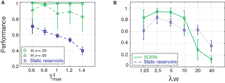
Figure 6. Influence of initial parameters on network performance. (A) Static reservoirs with different threshold settings are compared to SORNs with different network rates during learning (counting task, n = 10). (B) Role of connectivity on network performance (counting task, n = 14). Error bars indicate standard deviation.
In addition, we varied the number of synaptic connections per neuron (λW = 1.25, 2.5, 5, 10, 20, 40). Figure 6
B compares the prediction performance of networks with NE = 200, NU = 10,  ,
,  performing a counting task with n = 14. We find that a sparse connectivity is preferable both for static networks (blue) as well as SORNs (green). A high network connectivity induced seizure-like bursts of activity at the expense of computation (not shown). For a sparse connectivity SORNs perform better then the corresponding static reservoirs.
, performing a counting task with n = 14. We find that a sparse connectivity is preferable both for static networks (blue) as well as SORNs (green). A high network connectivity induced seizure-like bursts of activity at the expense of computation (not shown). For a sparse connectivity SORNs perform better then the corresponding static reservoirs.To summarize, SORN’s prediction performance: (a) is independent of the rate, criticality and performance of the initial static reservoir, (b) requires sparse network connectivity and (c) relies on a balanced representation of input spikes vs. reservoir spikes during learning.
The authors declare that the research was conducted in the absence of any commercial or financial relationships that could be construed as a potential conflict of interest.
This work was supported by the Hertie Foundation, grant PLICON (EC MEXT-CT-2006-042484) and GABA Project (EU-04330).
The Supplementary Material for this article can be found at: www.fias.uni-frankfurt.de/neuro/SupplementaryMaterial/lazarFrontiers2009.zip
- ^ Dynamics suitable for computation.