1
Institute for Clinical Neurosciences, Ludwig-Maximilians-Universität München, Munich, Germany
2
Graduate School of Systemic Neurosciences, Ludwig-Maximilians-Universität München, Munich, Germany
3
Laboratoire de Neurobiologie des Réseaux Sensorimoteurs, Centre National de la Recherche Scientifique, UMR 7060, Université Paris Descartes, Paris, France
4
Bernstein Center for Computational Neuroscience Munich, Munich, Germany
Intrinsic cellular properties of neurons in culture or slices are usually studied by the whole cell clamp method using low-resistant patch pipettes. These electrodes allow detailed analyses with standard electrophysiological methods such as current- or voltage-clamp. However, in these preparations large parts of the network and dendritic structures may be removed, thus preventing an adequate study of synaptic signal processing. Therefore, intact in vivo preparations or isolated in vitro whole brains have been used in which intracellular recordings are usually made with sharp, high-resistant electrodes to optimize the impalement of neurons. The general non-linear resistance properties of these electrodes, however, severely limit accurate quantitative studies of membrane dynamics especially needed for precise modelling. Therefore, we have developed a frequency-domain analysis of membrane properties that uses a Piece-wise Non-linear Electrode Compensation (PNEC) method. The technique was tested in second-order vestibular neurons and abducens motoneurons of isolated frog whole brain preparations using sharp potassium chloride- or potassium acetate-filled electrodes. All recordings were performed without online electrode compensation. The properties of each electrode were determined separately after the neuronal recordings and were used in the frequency-domain analysis of the combined measurement of electrode and cell. This allowed detailed analysis of membrane properties in the frequency-domain with high-resistant electrodes and provided quantitative data that can be further used to model channel kinetics. Thus, sharp electrodes can be used for the characterization of intrinsic properties and synaptic inputs of neurons in intact brains.
The standard method for characterizing properties of single neurons is the intracellular recording with glass micropipettes. Quantitative data on intrinsic and synaptic properties have been mainly obtained from recordings of neurons in culture or in slice preparations with low-resistant patch pipettes. The use of these low-resistant electrodes is required for the voltage clamp control of the membrane potential, which has been used for detailed analyses of ion channel kinetics (Neher and Sakmann, 1976
). However, a major drawback of these reduced preparations is that the surrounding neuronal network and the dendritic structures of individual neurons are partially removed, thus making this experimental approach less appropriate for an investigation of synaptic signal processing in complex circuits with feed-forward and feed-back loops, in particular where multiple and longer-range circuits contribute to this processing. Therefore, spatial and temporal aspects of synaptic signal processing in single neurons have been frequently studied in vivo or in isolated in vitro vertebrate whole brain preparations (e.g. Llinás and Yarom, 1981
; Hounsgaard et al., 1988
; Babalian et al., 1997
). In these preparations, intracellular recordings of neurons are most efficiently made with high-resistant (∼50–120 MΩ) sharp glass electrodes to maximize the success rate of impaling neurons.
The disadvantage of these high-resistant sharp electrodes, however, is that it is necessary to compensate the non-linear voltage drop across the electrode during intracellular current injections. The electrode compensation circuits that are implemented in most intracellular amplifiers usually treat the electrode as a simple linear RC circuit (resistor and capacitor). This procedure, however, is generally inadequate since sharp electrodes are often not simple RC elements and show current-dependent non-linear resistance changes (Brette et al., 2008
) that are difficult to describe quantitatively and thus impair a reliable use of bridge compensation (BC) or discontinuous current clamp (DCC) compensation (Moore et al., 1993
).
The present study describes a novel frequency-domain analysis of single neurons using offline electrode compensation that employs a Piece-wise Non-linear Electrode Compensation (PNEC) procedure to remove the separately measured electrode from the combination of both electrode and cell impedance. With this method it is possible to compensate for arbitrarily complex electrodes in frequency-domain data, which is an improvement to BC and DCC. Moreover it is also an improvement to the novel Active Electrode Compensation (AEC) method (Brette et al., 2008
) since the PNEC does not rely on the resistance linearity of the electrode and is independent of the ratio of electrode and membrane time constants, which do not need to be estimated mathematically from combined measurements of electrode and neuron.
The frequency-domain data provide current-dependent transfer functions, which can be used for the characterization of intrinsic membrane properties or to directly fit compartmental models with a comparable precision and reliability as those obtained from patch-clamp measurements (Booth et al., 1997
; Tennigkeit et al., 1998
; Roth and Häusser, 2001
; Erchova et al., 2004
; Taylor and Enoka, 2004
; Idoux et al., 2008
). Preliminary results have been published in abstract form (Rössert et al., 2008
).
Whole Brain Preparation
In vitro experiments were performed on isolated brains of six adult grass frogs (Rana temporaria) and complied with the “Principles of animal care”, publication No. 86–23, revised 1985 by the National Institute of Health. As described in previous studies (Straka and Dieringer, 1993
), animals were deeply anesthetized with 0.1% 3-aminobenzoic acid ethyl ester (MS-222), and perfused transcardially with iced Ringer solution (75 mM NaCl; 25 mM NaHCO3; 2 mM CaCl2; 2 mM KCl; 0.5 mM MgCl2; 11 mM glucose; pH 7.4). Thereafter, the skull and bony labyrinth were opened ventrally. After dissecting the three semicircular canals on each side, the brain was removed with all labyrinthine end organs attached to the VIIIth nerve. Subsequently, the brain was submerged in iced Ringer and the dura, the labyrinthine end organs and the choroid plexus covering the IVth ventricle were removed. In all experiments the forebrain was disconnected. Brains were used as long as 4 days after their isolation and were stored overnight at 6°C in continuously oxygenated Ringer solution (Carbogen: 95% O2, 5% CO2) with a pH of 7.4 ± 0.1. The brains were directly fixed with insect pins to the sylgard floor of a chamber (volume 2.4 ml) or glued with cyanoacrylate to a plastic mesh that was fixed to the floor of the recording chamber. The chamber was continuously perfused with oxygenated Ringer solution at a rate of 1.3–2.1 ml/min. The temperature was electronically controlled and maintained at 14 ± 0.1°C.
Classification of Neuronal Cell Types
External landmarks of the isolated frog whole brain served to identify the target sites for the intracellular recordings in the vestibular (Pfanzelt et al., 2008
) and the abducens nuclei (Straka and Dieringer, 1993
). Intracellularly recorded second-order vestibular neurons (2°VN) were identified by the activation of monosynaptic EPSPs following electrical stimulation of individual ipsilateral semicircular canal nerves (Straka et al., 1997
) with single constant current pulses (duration: 0.2 ms; threshold: ∼1–3 μA). These pulses were produced by a stimulus isolation unit (WPI A 360) and applied across suction electrodes whose opening diameters (120–150 μm) were individually adjusted. All 2°VN were classified as phasic or tonic neurons based on their responses to the injection of long, positive current steps (Straka et al., 2004
; Beraneck et al., 2007
; Pfanzelt et al., 2008
). Abducens motoneurons (AbMot) were identified by short-latency antidromic action potentials following electrical stimulation of the ipsilateral VIth cranial nerve with suction electrodes (diameter 100–150 μm). These neurons typically received a disynaptic crossed EPSP and an uncrossed IPSP following electrical stimulation of the bilateral horizontal canal nerve, compatible with previous results obtained after electrical stimulation of the entire VIIIth nerve (Straka and Dieringer, 1993
). Only 2°VN and AbMot with resting membrane potentials that were more negative than −55 mV were included in this study.
Complex Admittance Measurements with Sharp Microelectrodes
Sharp high-resistant glass microelectrodes for intracellular recordings were made with a horizontal puller (P-87 Brown/Flaming) using filament-containing borosilicate glass with pre-fire-polished ends (GB150F-8P, Science Products GmbH, Hofheim, Germany). Electrodes were filled with a 3-M solution of KCl or a mixture of 3 M KCl and 2 M KAc (1:10), which gave final resistances of 70–90 MΩ and 80–120 MΩ, respectively. Bath application of the potassium channel blocker 4-aminopyridine (4-AP; 20 μM) confirmed in one experiment the putative contribution of voltage-dependent potassium conductances (Wu et al., 2001
; Beraneck et al., 2007
) to the non-linear response properties of phasic 2°VN.
Voltage recordings and current injections were performed with a single-electrode clamp amplifier (SEC-05L, NPI Electronic GmbH, Tamm, Germany) in the “bridge balance” operation mode with no resistance or capacitance compensation. For A/D and D/A conversion a National Instruments acquisition card (PCI-6052E) was used with a PC (Intel Pentium 4, 1.9 GHz, Windows XP); the signals were sampled at 5 kHz. Recordings were done with a custom Matlab (Mathworks Corp.) program.
Responses of 2°VN and AbMot to a multi-sine current-clamp were measured at different membrane potentials. The multi-sine stimulus IMS was composed of 52–55 discrete frequencies of interest with a uniform stimulus amplitude and randomized phase spectra over a range of either 0.2–988.8 Hz or 0.2–1935.7 Hz (Idoux et al., 2008
). The constant magnitude was designed to drive the voltage responses uniformly at all frequencies of interest and the random phase spectrum was chosen to minimize the peak-to-peak dynamic amplitude of the stimulus waveform. The maximal half-amplitude of the multi-sine stimulus (hAmp = half of peak-to-peak amplitude) ranged from 0.4 to 1.2 nA with a duration of 6 or 12 s. In order to measure neurons at membrane potentials of interest (just below spike threshold), the multi-sine stimulus IMS was superimposed on a constant holding current Ihold, which preceded the multi-sine stimulus by 1.5 s. This holding current + multi-sine signal was the current clamp command or input current, Iref(t), (Figure 1
B) that led to an output voltage response V(t) (Figure 1
C). Each measurement consisted of two stimuli, where the second multi-sine stimulus, IMS, was multiplied by −1. A fast Fourier transform (FFT) was done on the difference of the two runs providing Iref(f) and V(f), respectively. The FFT, without windowing, has been computed on all N data points of Iref(f) and V(f), but only the frequencies present in the stimulus were used for the frequency-domain analysis.
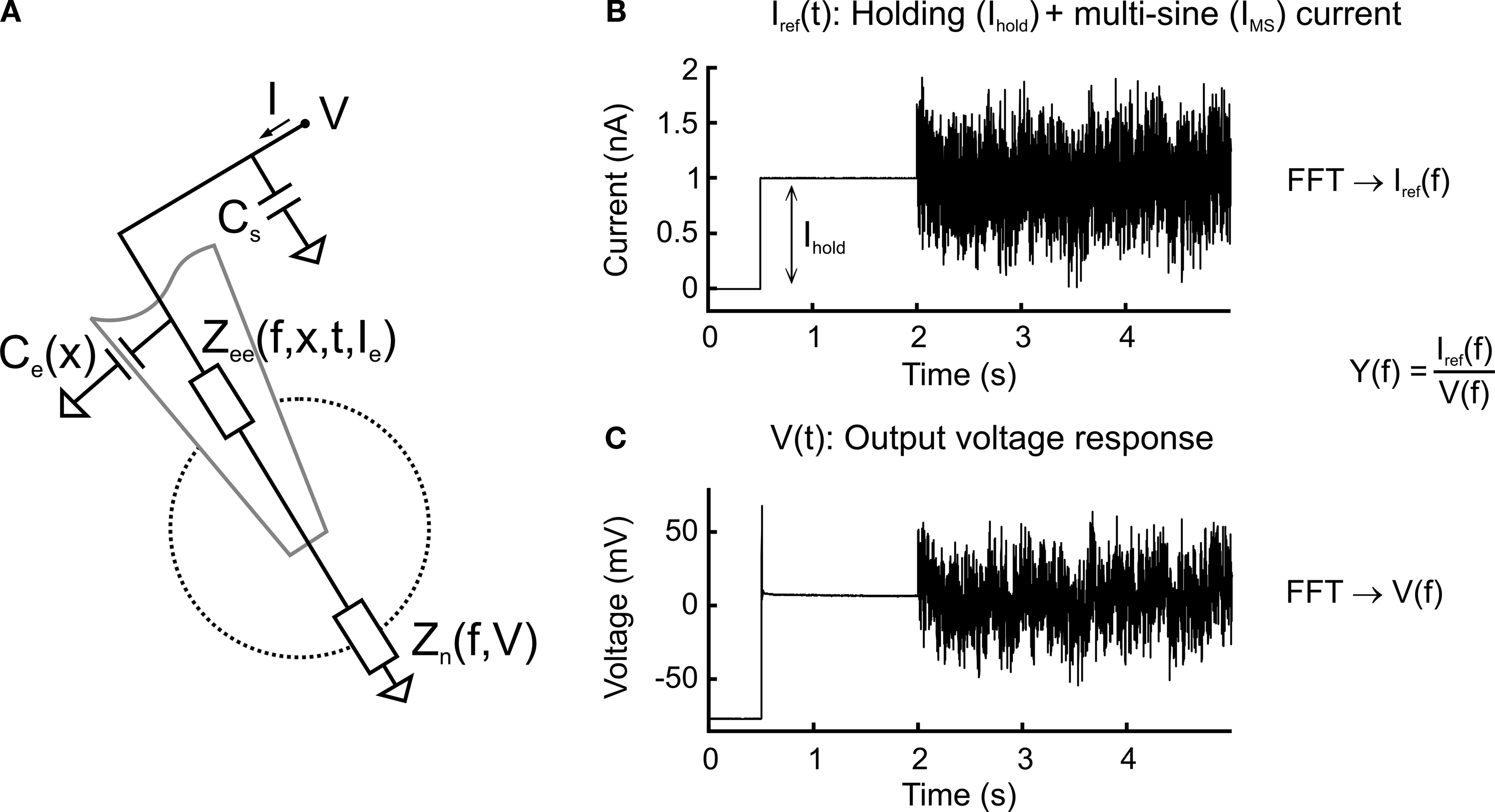
Figure 1. Circuit diagram and multi-sine measurement procedure. (A) Equivalent circuit diagram of a sharp electrode inside a neuron. The neuron is described as a frequency- and voltage-dependent impedance, Zn(f, V); the electrode is described as a frequency-, depth-, time- and current-dependent impedance Zee(f, x, t, Ie) serial to and a depth-dependent capacitance Ce(x) parallel to the neuron; additional constant parallel stray capacitance Cs of amplifier circuit. (B,C) Multi-sine current stimulus with discrete frequencies superimposed on a constant holding current, Ihold (B), injected through the electrode leading to a voltage response (C). Transformation into the frequency-domain by a fast Fourier transform (FFT) and division of the stimulus current by the voltage response leads to the admittance transfer function, Y(f).
The sum of the voltage responses V(t), VAveM, revealed the mean membrane potential and non-linear membrane effects, such as subthreshold responses or action potentials, as well as recurrent synaptic potentials evoked by the current injection during the two runs. Since the polarity of the stimulus alternated, the sum removed all coherent linear responses and thus VAveM is an excellent control for the quality of the measurement. The corresponding admittance transfer functions were computed as Y(f) = Iref(f)/V(f). Admittance extends the concept of conductance, taking into account dynamic effects by describing not only the relative amplitudes of the voltage and current, but also the relative phases. Admittance is expressed as a complex number Y(f) = G + jB with j being the imaginary unit and G the real part. It is the inverse of the impedance Z(f) = 1/Y(f), which is also a complex number, Z = R + jC with resistance R being the real part.
All transfer functions are shown as complex admittance or impedance Bode plots. In the complex admittance plots, the real part is shown on the x-axis, whereas the imaginary part is plotted on the y-axis. Each data point in this plot thus expresses a different frequency, starting with 0 Hz at the point (x,0). The length of a line that can be drawn between each point and (0,0) corresponds to the magnitude of the admittance at a given frequency, whereas the angle between this line and the horizontal x-axis is the phase shift between the response and the stimulation. Therefore the units of both axes of complex admittance plots are nano-Siemens (nS). All transfer functions after electrode subtraction are shown as the more common impedance Bode plots.
Since no electrode resistance or capacitance compensation was used, the resulting voltage response (Figure 1
C), and therefore the admittance transfer function, Y(f), refers to both the electrode and the neuron. In the following all admittance transfer functions are written as Yi with i being e, e + n or e + m indicating that the electrode was measured alone, within a neuron or with a neuronal model, respectively.
During intracellular measurements, the properties of the electrode are best described as a frequency-, depth- (electrode tip with respect to the surface of the Ringer solution in the recording chamber), time- and current-dependent serial impedance, Zee(f, x, t, Ie), and a depth-dependent capacitance, Ce(x), parallel to the neuron. In addition to this parallel electrode capacitance, a constant parallel stray capacitance, Cs, (Figure 1
A) is always present, i.e. the capacitance to ground at the input of the buffer operational amplifier (Molecular Devices, 2008
). In order to obtain reliable data on frequency responses of single neurons recorded with sharp electrodes, a procedure called Piece-wise Non-linear Electrode Compensation (PNEC) was developed to remove the electrode properties from the total response in the frequency-domain. To test the PNEC method a passive neuronal circuit model composed of a thin film resistance with Rm = 10 MΩ (Tolerance: ±0.02%) (Vishay Sfernice, Pennsylvania, USA) parallel to a polystyrene capacitor with Cm = 1 nF (Tolerance: ±1%) was used. For neuronal or model measurements the root-mean-square (RMS) error was computed separately for impedance magnitude and phase. The degree of electrode nonlinearity (λ) was calculated as the slope of the linear regression between injected current and the steady state electrode resistance (Brette et al., 2008
). Matlab (Mathworks Corp.) was used for computations. For time-domain simulations Simulink was used in combination with the SimPowerSystems Blockset to model the electrode and the passive neuron as electrical circuits. For AEC compensation the kernel computation and electrode kernel extraction was done using the latest Python implementation from http://audition.ens.fr/brette/HRCORTEX/AEC/AECcode.html
. For linear regression calculations the Matlab function “regress” was used. A model for the electrode has been created by fitting two distributed capacitances and resistances (RC’s) and a serial resistance and inductance (R–L) to the measured frequency response of an electrode using the Matlab function “lsqcurvefit”. Graphical presentations were made with Corel Draw (Corel Corporation Ltd.). Statistica 6.1 was used for the Wilcoxon matched pairs test.
Electrode Properties
Electrode properties were revealed by using a multi-sine analysis of the electrodes in the recording chamber and/or the tissue to determine the electrode transfer function, Ye. In contrast to a simple electrode model (constant parallel capacitance and resistance), which approximates a theoretically expected straight line on an admittance plot (red line in Figure 2
A1), the glass microelectrodes used for the present intracellular recordings show a complex frequency-dependent behavior of the real part (green and blue lines in Figure 2
A1) but an essentially linear behavior of the imaginary part, similar to a simple RC electrode model (Figure 2
A2). This behavior depended on the depth (x) of the electrode tip in the tissue and/or bath with respect to the level of the Ringer solution; in particular, the capacitance of the electrode increased with the depth (Figure 2
A2). Even though the resistance of sharp electrodes, filled with KCl or KAc, could fluctuate randomly within the range of minutes (Figure 2
B1), the shape of the admittance measurements and its imaginary component (Figure 2
B2) did not change over time. This spontaneous impedance change was considerably reduced, yet not absent when the electrode tip was inside a neuron. Injections of holding currents Ihold through the electrode radically changed the real part of the admittance measurements, but had little effect on its imaginary part (Figures 2
C1,C2). This behavior can be best seen in the corresponding impedance magnitude plot (Figure 2
C1 inset). Also, note that some sharp electrodes showed a resonance (* in Figure 2
C1 inset) at ∼50 Hz that occurred mostly for positive Ihold injections. Considering these results and taking into account the additional stray capacitance of the amplifier, the electrode transfer function can be described as
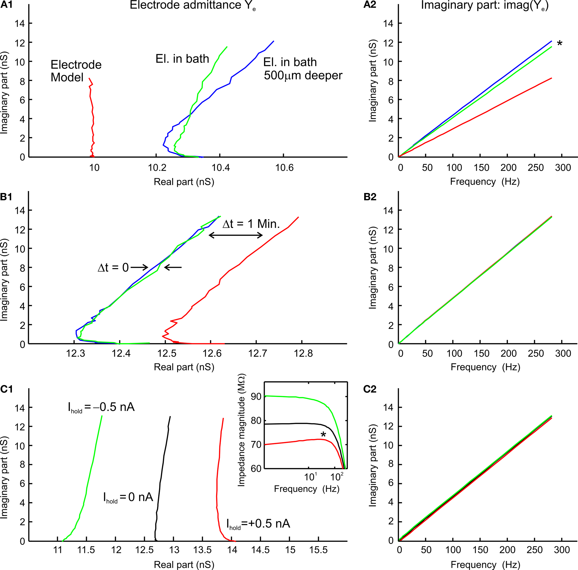
Figure 2. Multi-sine analysis of electrode properties with discrete frequencies plotted for the range from 0.2–300 Hz. (A1,A2) Admittance plots (A1) of the electrode model circuit with constant parallel capacitance and resistance (red line); admittance plots (A1) of KCl (3 M) filled electrode with the tip at 1.5 mm (green line) and 2 mm below the surface of the Ringer solution (blue line) show frequency-dependent changes of electrode properties influenced by the depth in the Ringer solution; plots of the imaginary part (A2) show that the electrode capacitance increases with increasing depth of the electrode tip in the bath (*); Ihold = 0 nA. (B1,B2) Admittance plots (B1) of three measurements of electrode properties in the recording chamber; measurements 1 and 2 were consecutive (green and blue lines), whereas the measurement 3 (red line) was taken 1 min later; note that the admittance fluctuates over time while the capacitance (B2) remains stable; Ihold = 0 nA. (C1,C2) Admittance plots (C1) of three electrode measurements with different holding currents Ihold = 0 nA (black line), −0.5 nA (green line), +0.5 nA (red line); injection of a constant current changes the real part of the electrode admittance response while the capacitance (C2) remains unchanged.

where Zee is the complex impedance of the electrode without an assumed passive capacitance. Thus, real(Ye) = real[1/Zee(f, x, t, Ie)] with an essentially frequency-, depth-, time- and current-dependency and imaginary(Ye) = j2πf[Ce(x) + Cs] + imagina-ry[1/Zee(f, x, t, Ie)], with the latter being dominated by a depth (x)-dependent electrode capacitance, Ce(x), plus Cs, the amplifier stray capacitance. Figures 2
A2,B2,C2 shows that the imaginary part of Ye depends linearly on the frequency and is thus almost completely described by j2πf[Ce(x) + Cs]. Therefore, the parallel capacitance, C = Ce + Cs can be estimated by fitting the function 2πfC to imaginary(Ye) using a linear regression. For all electrodes in the present study, the regression was highly significant (all R2 > 0.990).
Piece-Wise Non-Linear Electrode Compensation (PNEC) Procedure
Because of the particular complex electrode behavior, no electrode compensation (neither resistance nor capacitance compensation) was used, but a procedure called Piece-wise Non-linear Electrode Compensation (PNEC) was developed to subtract the electrode from the frequency-domain response offline after the measurements. The subtraction procedure involved measuring the electrode alone just after removing it from the neuron, but leaving it in the immediate vicinity (5–8 μm) of the cell and applying the same holding currents, Ihold, as used during the intracellular recording. The latter procedure was necessary because of the current-dependent non-linearities of the electrode. As indicated above, changes in the electrode impedance observed either spontaneously or after impalement (Brette et al., 2008
) are most likely due to partial blocking or unblocking of the micropipette tip as suggested by the finding that this behavior can be described by translating the real part of Ye along the real axis, which is equivalent to adding a conductance GT to the admittance Ye.
The impedance Zn of a passive neuron (resistance Rn and capacitance Cn) can be expressed by:
Thus at high frequencies, the neuron is shunted by its capacitance such that the electrode + neuron admittance measurement Ye+n should overlap with the electrode measurement Ye. Therefore, in order to compensate for the change in electrode impedance after leaving the neuron, Ye was translated along the real axis until it superimposed on Ye + n at high frequencies above ffit. For ffit, the frequency was chosen where the resistance of the neuron reaches 1% of its baseline resistance. Knowledge of the membrane time constant (τn) of a typical recorded neuron, ffit can thus be calculated by:
A τn = 2 ms, as measured in e.g. tonic and phasic 2°VN (Straka et al., 2004
) gives a ffit of 792 Hz, which was used in our experiments. With a typical neuronal resistance of 10 MΩ and typical electrode resistances of ∼100 MΩ the theoretical error calculated for the electrode resistance estimation is thus only ∼0.1% in our experiments.
After translating and determining the conductance GT, the electrode admittance measurements can be used to remove the electrode. Thus, this electrode compensation procedure, referred to as PNEC, is as follows:
(1) To estimate the conductance GT the error [real(GT + Ye) − real(Ye + n)]2 has to be minimized in the frequency range between ffit and the maximal frequency (fmax) measured. Since GT is real, the estimation of GT simplifies to:

(2) Fit 2πfC to imaginary(Ye), using linear regression, in order to remove the parallel electrode capacitance Ce(x), and amplifier stray capacitance Cs:

(3) Remove the serial impedance Zee(f, x, t, Ie) = (GT + Ye − j2πfC)−1 of the electrode:

The PNEC procedure has been performed with 19 neurons: the 19 electrodes showed a mean resistance of 85.5 ± 24.5 MΩ (mean ± SD) and a mean capacitance of 8.16 ± 2.01 pF; for GT an average of 0.76 ± 1.2 nS (mean ± SD) was estimated, which resulted in an RMS of 0.0375 ± 0.018 nS (mean ± SD; from ffit to fmax). The mean degree of nonlinearity (λ) could be evaluated in 12 electrodes and resulted in −2.56 ± 3.9 MΩ/nA (mean ± SD) which is comparable to nonlinearities found previously (Brette et al., 2008
).
Model Test of the Subtraction Procedure
Measuring a passive neuronal circuit model
The PNEC procedure was tested by measuring a passive neuronal circuit model (Rm = 10 MΩ, Cm = 1 nF), attached to the electrical path-to-ground, through a real electrode in the bath (Figure 3
A). Although this reproduces the serial resistive connection of an electrode to a real neuron, the electrode capacitance Ce is also serial to the neuron. Since the capacitance Ce is only parallel to the electrode it shunts only the electrode impedance, comparable to the parallel RC of neurons. Accordingly, at high frequencies the two measurements of Ye and Ye + m do not overlap and the translation conductance GT cannot be estimated. Thus GT was chosen for this model test in such a way that the resistance of the model neuron (10 MΩ) was correct at the lowest frequency after electrode subtraction. Figure 3
B shows the admittance plots with Ihold = 1 nA of electrode + model neuron (Ye + m) and the measured, but translated electrode (GT + Ye). Figures 3
C1,C2 illustrates that the impedance magnitude obtained after the PNEC procedure (orange lines) is in good agreement with the analytical values of the neuronal circuit model (green lines) (RMS: 0.22 MΩ), but shows an error for the phase at high frequencies (RMS: 21.5°) that will be corrected below by taking into account the complete serial connection of the electrode to the test model system. Thus, both the lack of overlapping Ye and Ye + m at high frequencies and the phase error are due to the serial connection of the electrode capacitance to the model. Since only the amplifier stray capacitance Cs is in parallel to the neuron model, its subtraction must be adapted to the test setup. This involves two individual subtractions of Cs = 4.4 pF that was estimated before by measuring a precision resistance, as follows:
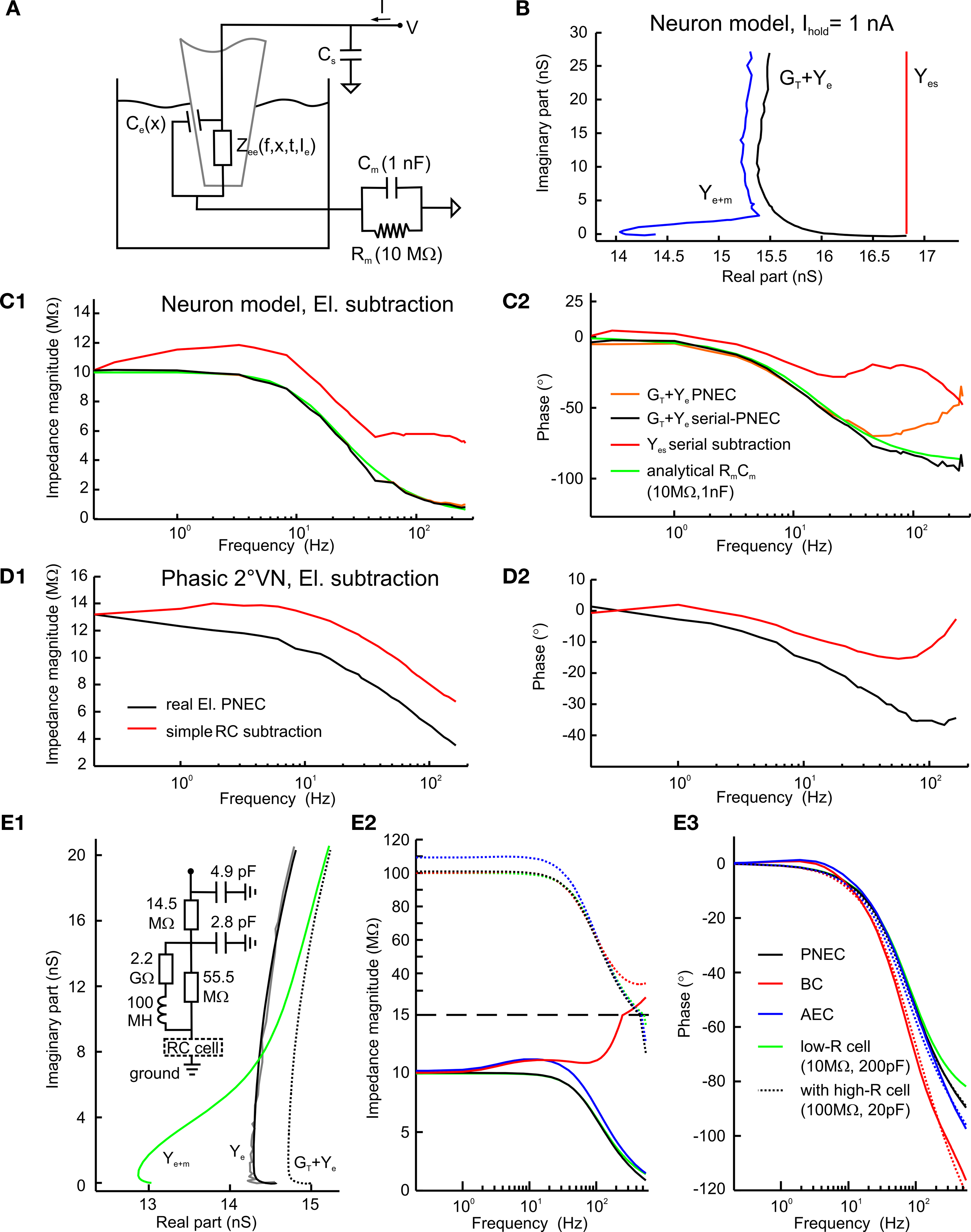
Figure 3. Model test of the Piece-wise Non-linear Electrode Compensation (PNEC) method. (A) Equivalent circuit diagram of the test setup with the electrode in the Ringer-filled recording chamber representing a parallel impedance Zee(f, x, t, Ie) and a capacitance, Ce(x), serial to a passive neuronal circuit model (Rm = 10 MΩ, Cm = 1 nF) attached to the electrical path-to-ground and a constant amplifier stray capacitance, Cs, parallel to the model. (B) Admittance plots of the corrected electrode alone GT + Ye (black line) of the electrode with an attached neuronal circuit model Ye + m (blue line) and the analytical response of a simple RC-type electrode model Yes (red line); Ihold = +1 nA, plotted frequency spectrum 0.2–485 Hz. (C1,C2) Bode plots of a passive neuronal circuit model using different electrode compensation methods on the combined measurement Ye + m: (a) electrode GT + Ye (orange lines) with PNEC, (b) electrode GT + Ye using serial-PNEC (black lines), (c) simple theoretical RC electrode, Yes, using serial subtraction (red lines) and (d) the analytical passive neuronal circuit model (green lines). Note that using the simple RC electrode compensation for the passive neuronal model shows a resonance that is solely an electrode compensation artifact; trace labels in (C2) also apply to (C1). (D1,D2) Results from the subtraction of a simple RC-type electrode (red lines) and using PNEC with the actual electrode (black lines) on the intracellular records of a phasic 2°VN; note that subtraction of a simple RC-type electrode also shows an incorrect resonance for the actual neuron that is caused by the above electrode artifact; trace labels in (D1) apply also to (D2). (E1) Time-domain simulation of PNEC, AEC and BC; admittance plots of an electrode with distributed capacities and parallel resistance and inductance (inset) Ye (black line) with parameters adjusted to mimic the behavior as measured in real electrodes (gray line), with an attached passive RC neuronal circuit model (10 MΩ, 200 pF) and reduced overall resistance Ye + m (green line) and shifted electrode GT + Ye + m (dotted line) prior to PNEC subtraction; plotted frequency spectrum 0–556.2 Hz. (E2,E3) Results after electrode compensation with a low resistance RC cell (low-R: 10 MΩ, 200 pF) (solid lines) or a high resistance RC cell (high-R: 100 MΩ, 20 pF) (dotted lines): simple BC (red) or AEC compensation (blue) causes electrode resonance artifacts in the impedance (E2) and phase (E3), while PNEC (black) complies well with the expected results (green); change of y-coordinate scale at 15 MΩ (dashed line) in (E2); trace labels in (E3) also apply to (E2).

With this serial-PNEC the phase errors can be eliminated and the obtained impedance magnitude and phase plots (Figures 3
C1,C2; black lines) match well with the analytical values for the neuronal circuit model (green lines) (RMS: 0.20 MΩ, 3.7°). This successful subtraction of electrode properties in the model test setup confirms that non-linear electrode properties can be appropriately taken into account during piece-wise linear measurements.
The critical need for correcting microelectrode measurements with measured electrode properties are illustrated by comparing the errors that result from assuming a simple RC electrode (Yes in Figure 3
B) although it has a resistance identical to the low-frequency (0.2 Hz) impedance of the real electrode and an identical capacitance. Figure 3
C shows that the serial subtraction, using adapted Cs subtraction as above, of a simple RC electrode (red lines) results in a considerable error and even suggests an incorrect resonance behavior because the real electrode has not been correctly taken into account (RMS: 3.40 MΩ, 41°). To further quantify the quality of fit, the correlations between the residuals (estimated magnitude and phase minus theoretical values) and the frequency have been analyzed for all three electrode subtractions. The residual error after BC or PNEC still showed a correlation with frequency for both magnitude and phase, but there was no significant correlation using serial-PNEC.
Similar errors using simple RC electrode compensation can also be seen in the data from recorded neurons. Using the PNEC procedure for a frog phasic 2°VN (Ihold = 0 nA; Figures 3
D1,D2) the magnitude and phase plots (black lines) suggest rather passive membrane properties. However, an incorrect subtraction using a simple RC electrode, with a resistance identical to the low-frequency impedance and capacitance identical to the real electrode, yields a considerable resonance (red lines) that however is an artifact due to the incorrect electrode compensation.
Comparison of PNEC, BC and AEC using an electrode model
Using a time-domain simulation in Matlab Simulink the performance of PNEC was compared to Bridge- (BC) and Active Electrode Compensation (AEC, Brette et al., 2008
). The frequency-domain behavior of a typical electrode (Figure 3
E1 gray plot) was modeled by using distributed capacitances and resistances (RC’s) reflecting the rightward bend in the electrode admittance plots at high frequencies and a serial resistance and inductance (R–L) in parallel to the last distributed RC to account for the resonant behavior at low frequencies. Thus the prominent electrode behaviors could be fitted (Ye in Figure 3
E1 black line) using two distributed RC’s of 14.5 or 55.5 MΩ and 4.9 or 2.8 pF, respectively and a R–L with 2.2 GΩ and 100 MH (Figure 3
E1 inset). To mimic the electrode resistance shift for the electrode inside the neuron, the resistance of the last RC was reduced from 55.5 MΩ to 53.5 MΩ when a purely passive RC-type neuron was added which, together with the electrode, produced the admittance response Ye + m as shown exemplarily for a low resistance neuron model (low-R: Rn = 10 MΩ, Cn = 200 pF) in Figure 3
E1 (green line).
For the simulation of BC, capacitance and resistance compensation have been directly implemented by simulating standard compensatory circuits (Molecular Devices, 2008
) in Simulink: resistance compensation has been set to the low-frequency resistance of the electrode and capacitance compensation has been used maximally just before ringing occurred. For AEC, only capacitance compensation has been simulated in Simulink and the resistance has been subtracted offline using the provided AEC procedure (Brette et al., 2008
). Prior to this simulation, the correct implementation of AEC could be confirmed using an electrode and neuron model as used in the simulations of Brette et al. (2008
; not shown).
The simulation has been realized for two types of neurons having a time constant of 2 ms: a low resistance neuron (low-R: Rn = 10 MΩ, Cn = 200 pF, solid lines) and a high resistance neuron (high-R: Rn = 100 MΩ, Cn = 20 pF, dotted lines), mimicking a large and small cell, respectively. Application of the PNEC procedure (with ffit = 792 Hz), i.e. shifting GT + Ye (Figure 3
1 dotted line) and subtracting the electrode admittance, results in only small errors (RMS: low-R: 0.2 MΩ, 3.4°; high-R: 1.6 MΩ, 3.5°) for the impedance magnitude and phase plots (black solid or dotted lines) when compared to the expected analytical results of the passive neuron (green solid or dotted lines) (Figures 3
E2,E3). In contrast, using BC (Figures 3
E2,E3 red solid or dotted lines) magnitude and phase errors (RMS: low-R: 10.5 MΩ, 20.1°; high-R: 7.6 MΩ, 21.0°) occur due to incorrect electrode compensation. For AEC (blue solid or dotted lines) (RMS: low-R: 0.8 MΩ, 6.7°; high-R: 5.5 MΩ, 7.2°), errors already occur at the low-frequency end due to the underestimation of the electrode resistance especially with the high resistance neuron, which results from the low ratio of electrode and membrane time constants. In addition, the inductive component of the electrode further complicates the correct electrode kernel estimation and results in a resonance that is an artifact due to the incorrect electrode compensation, which particularly can be seen in the low-R simulation. The simulations further show that the electrode compensation error in AEC is not solely dependent on the time constant ratio, as stated by Brette et al. (2008)
but also increases with the resistance of the cell. This is also the case for PNEC, but here the error can be further reduced by increasing ffit.
This comparison shows that the PNEC method is well suited to compensate for the complicated electrode behavior and yields better results compared to BC and even AEC. However, PNEC is also not perfect, since minor errors occur for the phase at very high frequencies, likely due to an insufficient compensation of distributed electrode capacitances. This suggests that PNEC is reliable at least up to ∼300 Hz for the estimation of neuronal frequency-domain transfer functions.
Measurement Results
Examples of electrode compensation for three different neuronal subtypes recorded with different holding currents (Ihold) in an isolated adult frog whole brain were used to illustrate the applicability of PNEC for typical neuronal recordings. Figure 4
A illustrates the electrode adjustment procedure for an AbMot at Ihold = +1 nA, which required a shift in the electrode admittance response, Ye, due to a difference in the electrode properties when it was removed from the neuron. As described above, the abscissa values were shifted prior to the subtraction in order for the curves to overlap at high frequencies above ffit indicated as GT + Ye. Electrode corrected magnitude and phase plots for this AbMot at other holding currents illustrate the marked potential dependence of the neuronal impedance including a pronounced resonance (Figures 4
B1,B2). Bode plot examples for previously described tonic (Figures 4
C1,C2) and phasic (Figures 4
D1,D2,E1,E2) 2°VN (Beraneck et al., 2007
) indicate that the membrane resonance properties reported for phasic 2°VN (* in Figures 4
D1,E1) are not an electrode artifact.
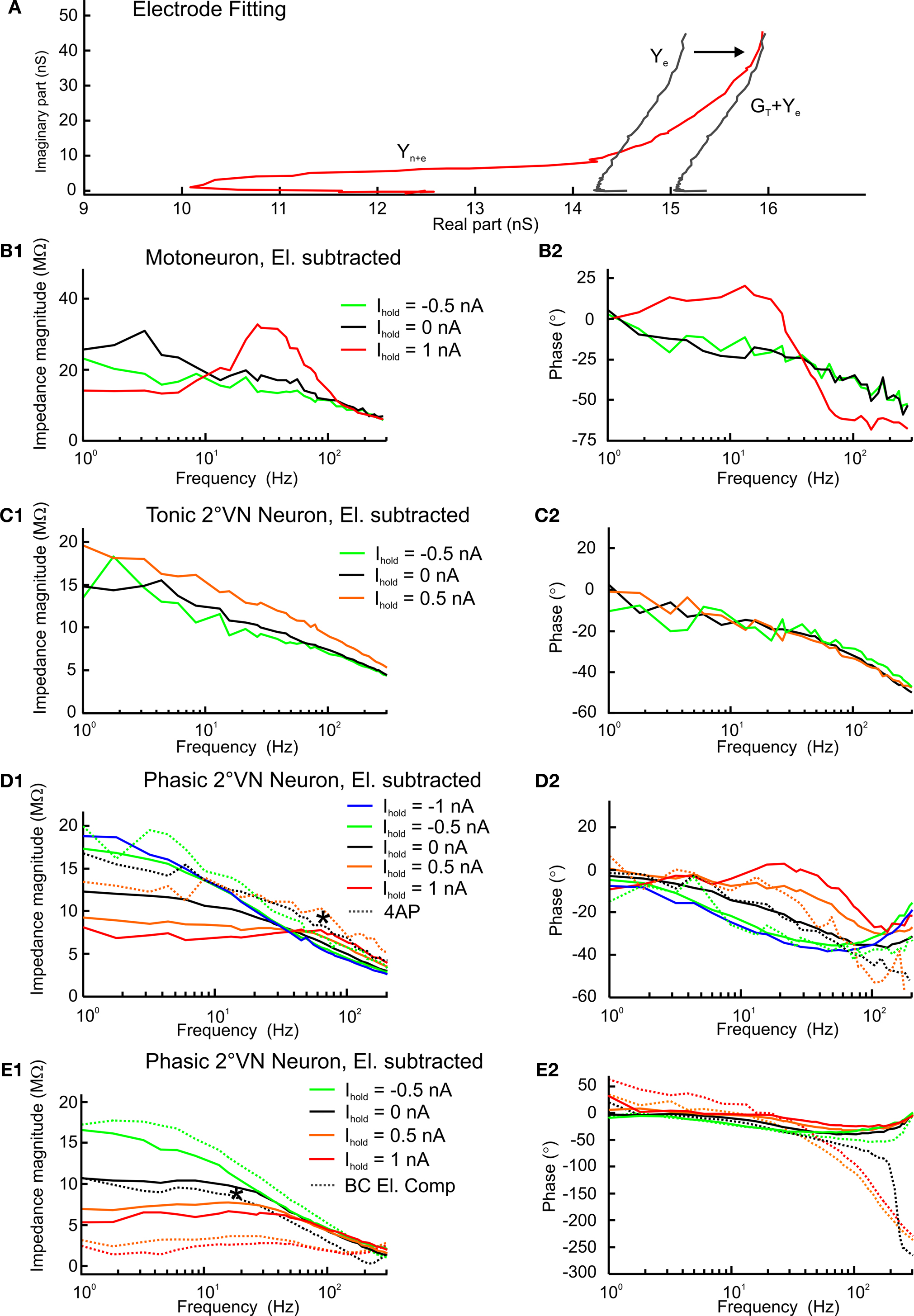
Figure 4. Electrode fitting and response dynamics of second-order vestibular neurons (2°VN) and abducens motoneuron (AbMot) using Piece-wise Non-linear Electrode Compensation (PNEC). (A) Electrode fitting procedure of the responses in an AbMot at Ihold = +1 nA; the electrode admittance Ye (solid line) changed after the electrode was removed from the neuron and was shifted (GT + Ye) in order to overlap at high frequencies with the properties of the electrode + neuron admittance Yn + e; plotted frequency spectrum 0.2–980 Hz. (B1,B2–D1,D2) Impedance profiles and corresponding phase relations of the responses at several holding currents (Ihold) of an AbMot (B1,B2), a tonic (C1,C2) and two different phasic 2°VN (D1,D2,E1,E2) after PNEC; responses of the phasic 2°VN shown in (D1,D2) were measured before and after bath application of 4-aminopyridine (4AP; 20 μM) [dotted lines in (D1,D2)] with PNEC; responses of the phasic 2°VN shown in (E1,E2) were measured after PNEC as well as during standard bridge compensation (BC) of the amplifier [dotted lines in (E1,E2)]; legends in (B1–E1) also apply to (B2–E2).
Multi-sine analysis allows direct visualization of the dynamic responses of functionally different neuronal phenotypes. For instance, the AbMot, which is plotted in Figures 4
B1,B2 revealed a high degree of resonance during depolarizing currents, most likely caused by an interaction of delayed rectifier potassium and sodium channels (Hutcheon and Yarom, 2000
). Frog tonic 2°VN have no membrane resonance behavior but exhibited an increasing impedance with membrane depolarization (Figures 4
C1,C2). This latter effect is likely caused by non-inactivating calcium or sodium inward currents as suggested previously (Beraneck et al., 2007
). In contrast, frog phasic 2°VN showed decreasing impedance and increasing resonance (* in Figures 4
D1,E2) with membrane depolarization due to the activation of low-threshold voltage-dependent ID-type potassium channels as reported earlier (Beraneck et al., 2007
). Furthermore, since ID-type potassium channels are specifically blocked by low concentrations of 4-AP (Wu et al., 2001
), bath application of 20 μM 4-AP during multi-sine measurements of a phasic 2°VN (dotted lines in Figures 4
D1,D2) leads to an increase in impedance magnitude for Ihold = 0 and Ihold = 0.5 nA.
To demonstrate the errors induced by insufficient bridge compensation (BC), another phasic 2°VN (Figures 4
E1,E2) has been additionally measured during standard BC from the amplifier (dotted lines). While both compensation types match fairly well at the lowest frequencies for Ihold = 0 and −0.5 nA, the measurements at depolarized membrane potentials show an overcompensation due to electrode rectification. Furthermore incorrect compensation of the distributed electrode RCs in BC leads to bends in the magnitude and large jumps in the phase at higher frequencies (∼200 Hz).
To compare the PNEC method with standard bridge compensation (BC), both techniques have been applied in a total of 11 neurons at Ihold = 0 nA. Since the measurements were made at resting membrane potential, these neurons presumably behave like passive RC circuits with an impedance of Yn = Gn + j2πfCn. Thus Cn can be estimated by fitting j2πfCn to imaginary(Y) using a linear regression and Gn = mean[real(Y)], where Y is the measured neuronal admittance after either PNEC or BC compensation. The root-mean-square error of this fit is calculated as  This test resulted in a better RMS for PNEC, median of RMS: 0.0458 μS, compared to BC, median of RMS: 0.1818 μS (difference highly significant with p = 0.0076, Wilcoxon matched pairs test).
This test resulted in a better RMS for PNEC, median of RMS: 0.0458 μS, compared to BC, median of RMS: 0.1818 μS (difference highly significant with p = 0.0076, Wilcoxon matched pairs test).Test of Piece-Wise Linearity
Control experiments were performed to evaluate the validity of the assumption of piece-wise linearity for PNEC. Measurements of the electrode alone with different multi-sine half-amplitudes (hAmp = half of peak-to-peak amplitude of multi-sine stimulus; hAmp = 1 nA and hAmp = 0.5 nA) showed that, apart from the time-dependent translational shift of the electrode, the frequency response itself (e.g. Ihold = +0.5 nA in Figure 5
A) does not change with increasing amplitude. Nevertheless, as shown before, frequency responses are significantly affected by the holding Ihold current level (compare with Brette et al., 2008
). A further indication of the linearity over the range of multi-sine amplitudes is the successful test subtraction procedure (Figures 3
A–C2). Thus, this is a piece-wise linear analysis of two non-linear elements, the neuron and the electrode, both of which show marked non-linearities at different holding current levels. The non-linear effects of the neuron itself are due to its voltage-dependent ion channels. Measuring AbMot with an Ihold = 0 nA and multi-sine currents with three different half-amplitudes of hAmp = 0.4 nA, 0.6 nA and 0.8 nA showed that, apart from some fluctuations in the phase using the largest multi-sine current (hAmp = 0.8 nA), all measurements yield identical results (Figures 5
B1,B2). The source of these phase fluctuations using hAmp = 0.8 nA could be pinpointed by the observation of VAveM, which indicated that the multi-sine current triggered a few spikes (not shown). This result illustrates an important restriction required for most linearization methods, namely that the multi-sine amplitude should be chosen such that it is small enough not to trigger action potentials, but large enough to have a reasonable signal-to-noise ratio.
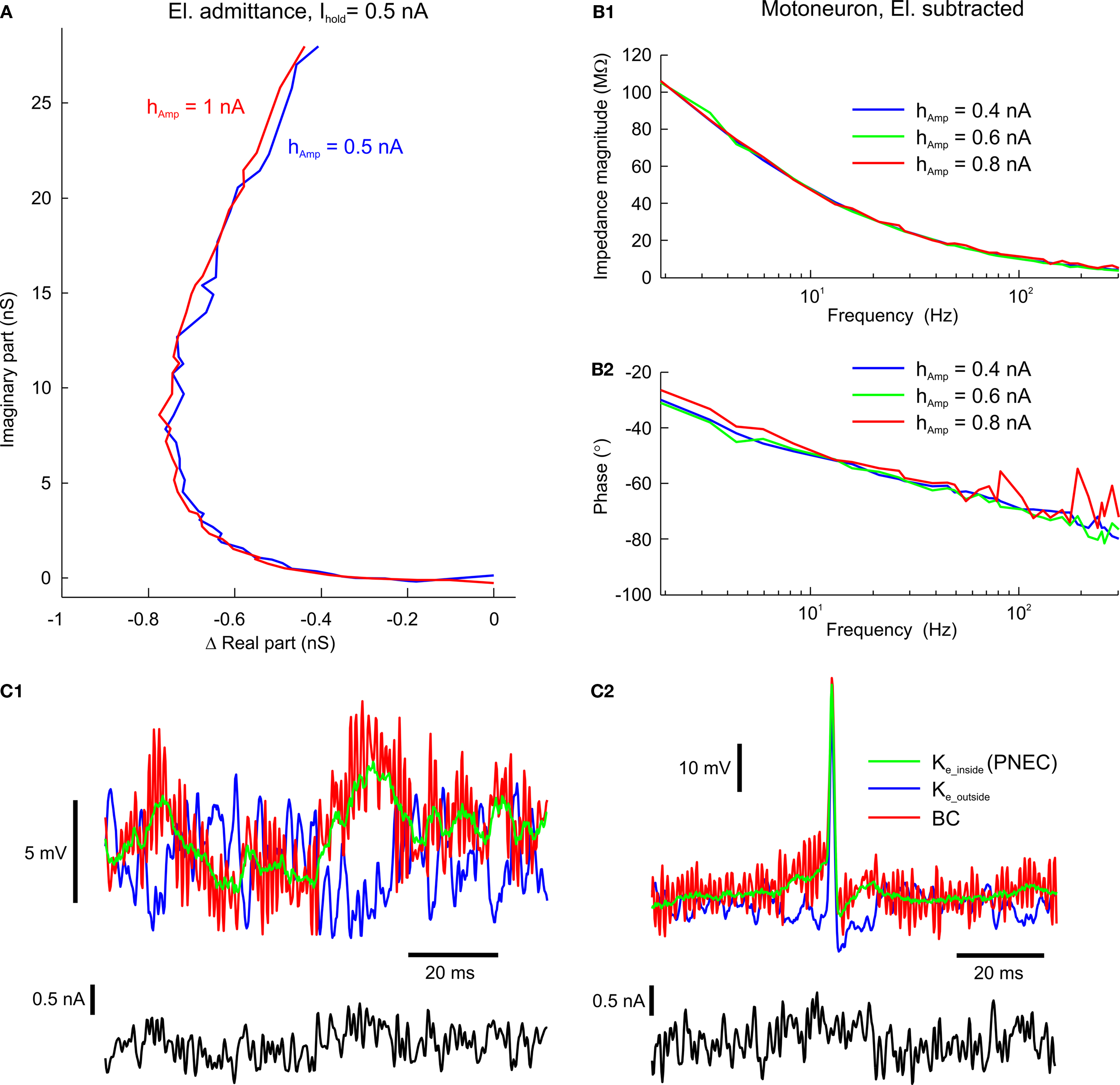
Figure 5. Test of piece-wise linearity and offline compensation in time-domain measurements. (A) Admittance plot of the electrode properties at half peak-to-peak multi-sine current amplitudes of hAmp = 0.5 nA (blue line) and hAmp = 1 nA (red line); real part is shown as relative conductance to correct for the temporal fluctuation; plotted frequency spectrum 0.2–625 Hz. (B1,B2) Bode plots of the impedance profiles of an AbMot at Ihold = 0 nA and peak-to-peak multi-sine current half amplitudes of 0.4 nA (blue lines), 0.6 nA (green lines) and 0.8 nA (red lines) after using Piece-wise Non-linear Electrode Compensation (PNEC). (C1,C2) Time-domain off-line subtraction of electrode voltage responses in a phasic (C1) and a tonic 2°VN (C2) during multi-sine stimulation (black traces) using the PNEC procedure for kernel determination (green traces), simple constant resistance/bridge compensation (red traces) and uncorrected electrode kernels Ke_outside, measured outside the cell (blue traces).
Outlook: Compensation in Time-Domain Measurements
Since we are considering piece-wise linear systems, the frequency-domain data can be translated into the time-domain, and therefore it is also possible to use the present PNEC framework to dissociate electrode from neuronal responses for arbitrary stimuli, as long as the current amplitude of the latter remain in the linear range. In the following, a method is presented that allows the determination of the electrode kernel for electrode compensation in the time-domain using the described PNEC framework. For this purpose, multi-sine measurements of the electrode alone, outside the cell, were used to calculate the electrode kernel Ke_outside via cross-correlation between input current and output voltage (similar to Brette et al., 2008
). These electrode kernels however differ from the real electrode kernel inside the cell and were thus corrected using the conductance GT, estimated via the second measurement inside the cell, as described before. For this correction, the kernel Ke_outside was transformed into the frequency domain via FFT, shifted by GT, which was estimated using the first step of PNEC, and transformed back into the time-domain using an inverse FFT:

This corrected electrode kernel Ke_inside can be further used to compute the electrode voltage by convolving it with the injected current Ie:

However, since no electrode capacitance compensation was used in our experiments, the measured electrode + neuronal voltage Ve + n and the computed electrode voltage Ve were low-pass filtered by the electrode, but could be corrected using voltage deconvolution (Richardson and Silberberg, 2008
) with:

Here by τ = RC, with R being the impedance at the lowest frequency and C estimated from imaginary(Ye) during the PNEC procedure.
After application of this voltage deconvolution to Ve + n and Ve, the neuronal voltage response could be computed as Vn = Ve + n − Ve. The results of this procedure were applied offline to the responses of a phasic (Figure 5
C1, green traces) and a tonic 2°VN (Figure 5
C2, green traces), measured during multi-sine stimulation (Figures 5
C1,C2 black traces) with current amplitudes in the linear range, showed that the high-frequency electrode voltage had been removed leaving a low-frequency neuronal voltage, since the injected current was filtered by the neuronal time constant. Compensation of electrode voltage under noisy current stimulation is a demanding task for each electrode compensation mechanism: using a simple constant resistance R for the estimation of the electrode voltage and thus subtracting Ve = RIe, equivalent to standard bridge compensation, leads to insufficient electrode compensation (Figures 5
C1,C2 red traces) since small errors in the estimation of the electrode voltage result in high-frequency electrode artifacts (compare with Brette et al., 2008
, supplemental data). In addition, using the uncorrected electrode kernels Ke_outside for offline compensation (Figures 5
C1,C2 blue traces) causes an incorrect estimation of Vn since the overall electrode resistance is overestimated in this case.
In essence, this indicates that the PNEC procedure can be used for a direct estimation of the electrode kernel and offline subtraction of the electrode voltage in the time-domain. For some applications, such as voltage-, or dynamic-clamp experiments, an offline compensation, however, is not sufficient. Nevertheless it is clear that the PNEC procedure to determine the electrode kernel can also be used in combination with online AEC (Brette et al., 2008
), as long as the electrode is measured twice: before entering a neuron and inside a neuron. It should also be noted, that for online AEC using the PNEC electrode kernel estimation it is more convenient to use capacitance compensation from the amplifier, as also suggested for normal AEC (Brette et al., 2008
), which supersedes the voltage deconvolution step.
The new Piece-wise Non-linear Electrode Compensation (PNEC) method provides a way to take into account the non-linear effects of arbitrarily complex electrode properties in the frequency-domain, without online control or compensatory manipulations during the recording. This not only avoids the uncertainties involved in separating the effects of the electrode compared to those of the neuron, but also the frequent errors caused by improper online compensation, which is difficult if not almost impossible to correct afterwards.
In contrast to the Active Electrode Compensation (AEC) method described recently (Brette et al., 2008
) the electrode properties in our PNEC method are not estimated from an electrode + neuron measurement, but are measured separately for each injected current step and corrected afterwards from the frequency-domain data, thus allowing the compensation of slow non-linearities caused by each current step. This compensation procedure is thus not only independent of electrode- and membrane-time constant ratios but also insensitive to resistance non-linearities of the electrode, which is not the case with AEC. Furthermore, using a simulation, it appears that the AEC electrode kernel estimation procedure is inaccurate especially when the electrodes show an inductive/resonating behavior, which however is not a problem for our PNEC procedure.
Frequency responses of neurons have been determined with low-resistant patch pipettes as well as with high-resistant sharp electrodes, but always using standard electrode compensation techniques. While this is not a problem for low-resistant patch pipettes, caution is advised when using high-resistant sharp electrodes and control experiments with the electrodes should be conducted prior to each experiment (see Moore et al., 1993
). A previous work using high-resistant sharp electrodes (Gutfreund et al., 1995
) states that their electrode impedance was frequency independent in the range of 0–50 Hz, which suggests the following: first, the maximum frequency was sufficiently low in order not to cause errors due to distributed electrode RCs and second, since slices were used, the electrode tips were not immersed as deeply into the bath or brain tissue compared to whole brain recordings which reduces the low frequency inductive/resonating behavior (compare Figure 2
A1, blue and green lines).
It is important to emphasize that the piece-wise linear electrode properties shown here, such as the resonant electrode behavior, should not be understood as a general description of all glass micro-pipettes but should rather be considered as an example showing that PNEC is capable of compensating any arbitrarily complex electrodes in the frequency-domain response.
It should also be noted that the offline PNEC method presented here was specifically developed for a frequency-domain analysis. Nevertheless, we could show that the PNEC framework can be used for determination of the electrode kernel and offline subtraction of the electrode voltage in the time-domain. Furthermore this kernel estimation procedure can be used with online AEC (Brette et al., 2008
) as long the electrode is measured before entering a cell. The advantage of the combination of the two methods helps avoiding errors that result from the standard AEC electrode kernel estimation.
PNEC is a piece-wise linear method that requires an amplitude of the injected multi-sine current that does not trigger action potentials. Thus, the holding currents Ihold have to be selected to drive the neuron either to a sub-threshold membrane potential or to a membrane potential where spiking does not occur due to sodium channel inactivation. As in other compensation methods, the present technique relies on combining distributed capacities of the electrodes. Based on the simulations, a frequency of ∼300 Hz is the upper limit for reliable neuronal impedance measurements with sharp, high-resistant electrodes using PNEC, which covers the important frequency range for most neuronal transfer functions. PNEC is capable of estimating neuronal transfer functions with high-resistant sharp electrodes and is thus a reasonable tool to correlate intrinsic membrane properties with synaptic signal processing in functionally intact whole brain preparations. The resulting neuronal representation in the frequency-domain can be used to analyze membrane properties and the different contributions of ion channels (Hutcheon and Yarom, 2000
). It even is feasible to use these neuronal frequency responses to obtain Hodgkin–Huxley type models (Moore et al., 1995
; Murphey et al., 1995
; Booth et al., 1997
; Tennigkeit et al., 1998
; Saint Mleux and Moore, 2000
; Roth and Häusser, 2001
; Erchova et al., 2004
; Taylor and Enoka, 2004
; Idoux et al., 2008
). In combination with synaptic activation (e.g. Pfanzelt et al., 2008
) it is now possible to estimate the synaptic signal processing properties and transfer functions of individual neurons within an entire network.
The authors declare that the research was conducted in the absence of any commercial or financial relationships that could be construed as a potential conflict of interest.
The authors acknowledge the help of Tobias Kohl in part of the neuronal recordings. This research was supported by the CNRS, CNES and BMBF (01GQ0440). Christian Rössert received a PhD-grant from the Bayerische Forschungsstiftung.
Molecular Devices (2008). The Axon Guide, A Guide to Electrophysiology & Biophysics Laboratory Techniques (Online). Available at: http://www.moleculardevices.com/pdfs/Axon_Guide.pdf
, Version 2500-0102 Rev. C.