Much of our behavior is shaped by feedback from the environment. We repeat behaviors that previously led to rewards and avoid those with negative outcomes. At the same time, we can learn in many situations without such feedback. Our ability to perceive sensory stimuli, for example, improves with training even in the absence of external feedback.

Guggenmos et al. hypothesized that this form of perceptual learning may be guided by self-generated feedback that is based on the confidence in our performance. The general idea is that the brain reinforces behaviors associated with states of high confidence, and weakens behaviors that lead to low confidence.

To test this idea, Guggenmos et al. used a technique called functional magnetic resonance imaging to record the brain activity of healthy volunteers as they performed a visual learning task. In this task, the participants had to judge the orientation of barely visible line gratings and then state how confident they were in their decisions.

Feedback signals derived from the participants’ confidence reports activated the same brain areas typically engaged for external feedback or reward. Moreover, just as these regions were previously found to signal the difference between actual and expected rewards, so did they signal the difference between actual confidence levels and those expected on the basis of previous confidence levels. This parallel suggests that confidence may take over the role of external feedback in cases where no such feedback is available. Finally, the extent to which an individual exhibited these signals predicted overall learning success.

Future studies could investigate whether these confidence signals are automatically generated, or whether they only emerge when participants are required to report their confidence levels. Another open question is whether such self-generated feedback applies in non-perceptual forms of learning, where learning without feedback has likewise been a long-standing puzzle.

Learning is an integral part of our everyday life and necessary for survival in a dynamic environment. The behavioral changes arising from learning have quite successfully been described by the reinforcement learning principle (Sutton and Barto, 1998), according to which biological agents continuously adapt their behavior based on the consequences of their actions. Thus, reinforcement learning models and most other learning models depend on feedback from the environment. Yet, there are important instances of learning where no such external feedback is provided, challenging the generality of these learning models in shaping our behavior.

A well-studied case of learning is the improvement of performance in perceptually demanding tasks through training or repeated exposure (Gibson, 1963). Such perceptual learning has repeatedly been demonstrated to occur without feedback (Herzog and Fahle, 1997; Gibson and Gibson, 1955; McKee and Westheimer, 1978; Karni and Sagi, 1991) and is therefore ideally suited as a test case to study learning in the absence of external feedback. Previous work has emphasized the role of reinforcement learning in perceptual learning (Kahnt et al., 2011; Law and Gold, 2009). However, these accounts were based on perceptual learning with external feedback and therefore cannot account for instances in which learning occurs without external feedback. Here, we pursued the idea that, in the absence of external feedback, learning is guided by internal feedback processes that evaluate current perceptual information in relation to prior knowledge about the sensory world. We reasoned that introspective reports of perceptual confidence could serve as a window into such internal feedback processes. In this scenario, low or high confidence would correspond to a negative or positive self-evaluation of one’s own perceptual performance, respectively. Accordingly, confidence could act as a teaching signal in the same way as external feedback in normative theories of reinforcement learning (Daniel and Pollmann, 2012; Hebart et al., 2014). Applied to the case of perceptual learning, a confidence-based reinforcement signal could serve to strengthen neural circuitry that gave rise to high-confidence percepts and weaken circuitry that led to low-confidence percepts, thereby enhancing the quality of future percepts.

We tested this idea in a challenging perceptual learning task, in which participants continuously reported their confidence in perceptual choices while undergoing functional magnetic resonance imaging (fMRI). No external feedback was provided; instead, confidence ratings were used as a proxy of internal monitoring processes. To account for perceptual learning in the absence of feedback, we devised a confidence-based associative reinforcement learning model. In the model, confidence prediction errors (Daniel and Pollmann, 2012) serve as teaching signals that indicate the mismatch between the current level of confidence and a running average of previous confidence experiences (expected confidence). Based on recent evidence of confidence signals in the mesolimbic dopamine system (Daniel and Pollmann, 2012; Hebart et al., 2014; Schwarze et al., 2013), we hypothesized to find neural correlates of confidence prediction errors in mesolimbic brain areas such as the ventral striatum and the ventral tegmental area. Since confidence prediction errors act as a teaching signal in our model, we hypothesized that the strength of these mesolimbic confidence signals should be linked to individual perceptual learning success.

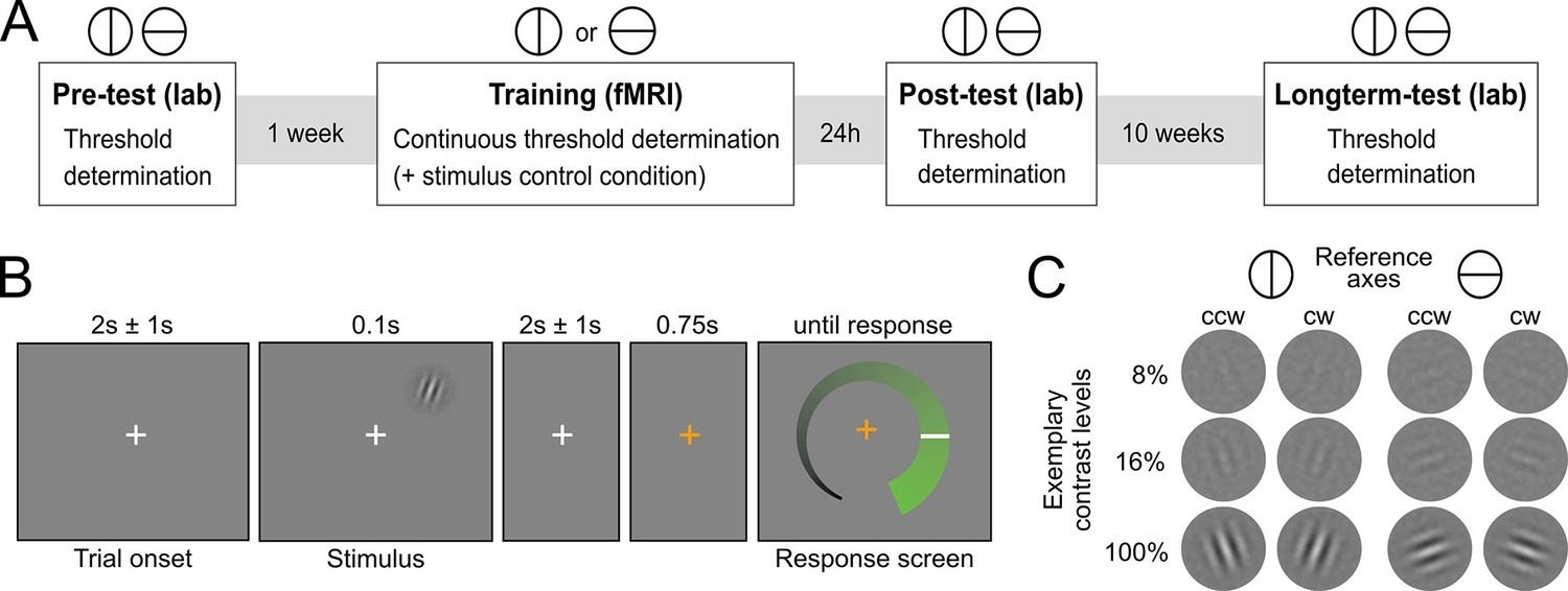
Human participants (N=29) learned to detect the orientation of peripheral noise-embedded Gabor patches relative to a horizontal or vertical reference axis while undergoing functional magnetic resonance imaging (fMRI). Overall, the experiment comprised four sessions: (i) an initial behavioral test session to establish participants’ baseline contrast thresholds for a performance level of 80.35% correct responses, (ii) an intensive perceptual learning session (training) in the MRI scanner with a continuous threshold determination, and two behavioral post-training test sessions to examine (iii) short-term and (iv) long-term stimulus-specific training effects (Figure 1A). While the training session was based on one reference axis, all test sessions comprised a contrast threshold determination for both reference axes. The training session additionally included a control condition in interleaved presentation, for which the contrast was kept constant to enable an exploratory multivariate analysis of changes in neural stimulus representation. The Gabor stimuli were flashed briefly in the upper right quadrant and participants had to judge their orientation with respect to the current reference axis (Figures 1B,C). Eyetracking ensured that participants maintained fixation throughout the training session (Figure 2—figure supplement 1). Importantly, participants did not receive external cognitive or rewarding feedback during the entire experiment. Rather, in addition to their choice, they reported their confidence about the stimulus orientation on a visual analogue scale (for a verification of accurate usage, see Figure 2—figure supplement 2). The confidence reports were used to compute the internal feedback in our model on a trial-by-trial basis.

Figure 1

Download asset Open asset

Stimulus-specific perceptual learning

To establish stimulus-specific perceptual learning, we compared perceptual thresholds in pre- and post-experimental sessions between the trained and untrained reference axis (Figure 2A). The contrast thresholds improved for the trained (t₂₈ = 6.73, p < 0.001, two-tailed), but not for the untrained reference axis (t₂₈ = 0.41, p = 0.68; interaction of training × time: F_1,28 = 14.2, p < 0.001), demonstrating clear and specific effects of perceptual learning. These stimulus-specific training effects could still be detected 10 weeks later (F_1,28 = 4.3, p = 0.047), indicating long-term stability and thus demonstrating a key characteristic of perceptual learning (Karni and Sagi, 1993). To test whether the effects of learning could already be detected during the training session, we linearly fitted the contrast thresholds across trials in the critical constant performance condition. The analysis showed that contrast threshold consistently decreased across runs (linear slope: −0.006 ± 0.002, t₂₈ = −2.38, p = 0.024), from 8.64% ± 0.47 (mean ± SEM) in the first training run to 7.68% ± 0.52 in the last training run.

Figure 2 with 2 supplements see all

Download asset Open asset

To assess whether participants adequately used the continuous confidence rating scale during training, the relationship between reported confidence and performance (proportion correct) was analyzed by means of a sliding window across sorted confidence values. The performance increased monotonically with confidence (main effect of percentile: F_22,2442 = 5.76, p < 0.001, one-way ANOVA with repeated measures), approaching chance at low levels of confidence, without showing ceiling effects at high levels of confidence (Figure 2B). This pattern indicates a close link between the decisional certainty of the choice and the reported confidence and shows that confidence represents valuable self-generated feedback.

A confidence-based model of perceptual learning

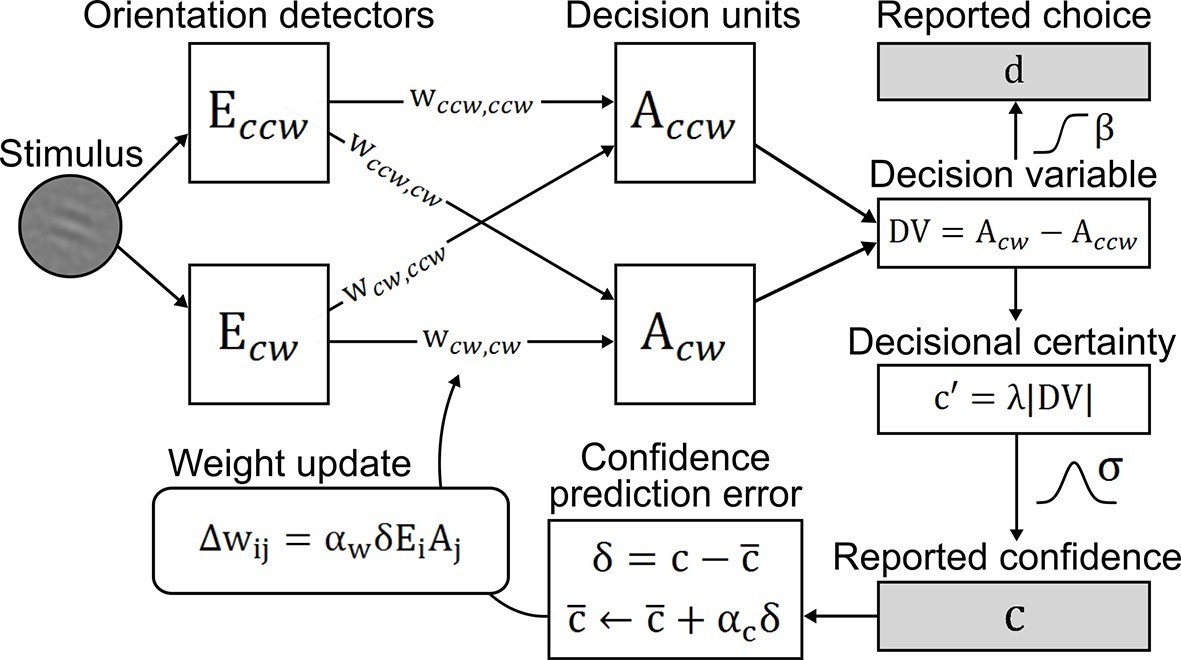
To account for perceptual learning without external feedback, we devised an associative reinforcement learning model with confidence as internal feedback (Figure 3). Learning in this model was guided by the combination of a confidence-based reinforcement signal and Hebbian plasticity, inspired by the previously proposed three-factor learning rule (dopaminergic reinforcement signal, pre-synaptic activity, post-synaptic activity) for neural plasticity in the mesolimbic system (Reynolds et al., 2001; Schultz, 2002). Our model assumes that observers improve perceptual performance by optimizing a filter on incoming sensory evidence. The filter is represented by two components: signal weights for clockwise (cw) and counterclockwise (ccw) stimulus orientation (w_ccw,ccw; w_cw,cw), connecting orientation energy detectors E_ccw/cw to decision units A_ccw/cw with same orientations; and noise weights (w_ccw,cw; w_cw,ccw), connecting detectors E_ccw/cw to decision units A_cw/ccw with opposing orientations. The clockwise and counterclockwise orientation energy contained in the stimuli is computed by a simple model of primary visual cortex (Petrov et al., 2005). The weighted sums of E_ccw/cw determine the activities of decision units A_cw/ccw which, in a next step, are integrated in a decision value DV = A_cw − A_ccw. DV translates into probabilities for clockwise or counterclockwise choices via a softmax action selection rule, and to the model’s equivalent of confidence—decisional certainty—through its absolute value. Finally, perceptual learning is based on an associative reinforcement learning rule with two separate components: a reinforcement component utilizes a confidence prediction error (CPE; denoted as δ) as internal feedback, representing the mismatch between current confidence and a long-term estimate of expected confidence (via a learning rate α_c); and a Hebbian component ensures that the weights are updated in proportion to how strongly orientation detectors and decision units co-activate. In addition, a learning rate α_w accounts for inter-individual differences in learning speed. Figure 3—figure supplement 1 provides an exemplary time slice of one participant's behavioral reports and accompanying model variables.

Figure 3 with 1 supplement see all

Download asset Open asset

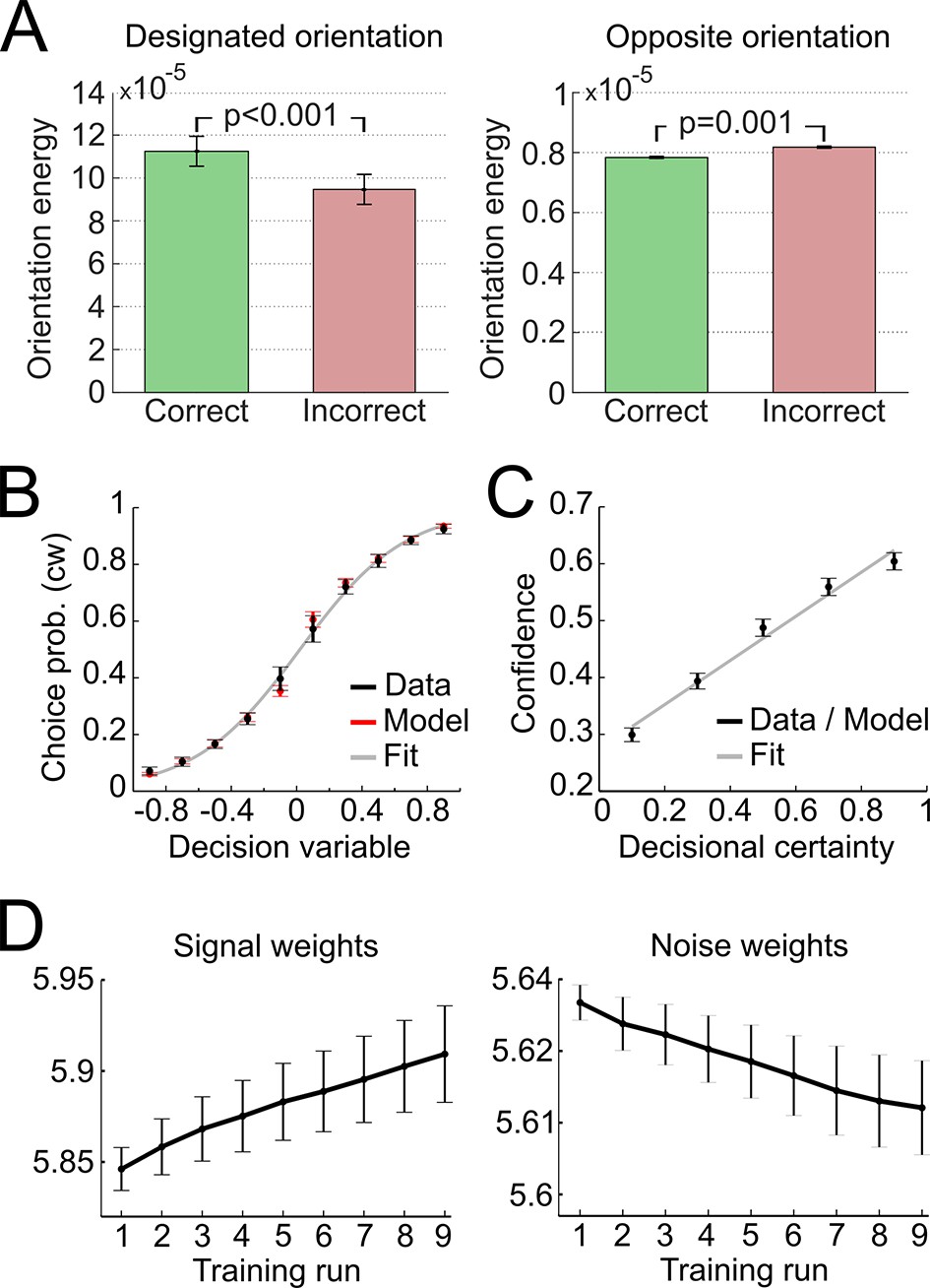
In a first step, we validated the representational subsystem by computing the average energy content for a range of spatial frequencies (one octave above and below the actual frequency of 1.25 cycles/degree) and for a range of orientations (−40° to +40° relative to the reference axes). As expected, the energy content was higher for the spatial frequency and orientations used to generate the Gabor patches relative to other frequencies and orientations (Figure 4—figure supplement 1). Further, when orientation energy was computed separately for correct and incorrect responses, the energy for designated orientations (i.e., the orientations used to generate the Gabor patches) was higher for correct than for incorrect responses (t₂₈ = 8.1, p < 0.001), whereas the energy for opposite orientations (i.e., ∓20° if ±20° was presented) was lower for correct than for incorrect responses (t₂₈ = −3.6, p = 0.001) (Figure 4A). This pattern demonstrated that the varying orientation energy was directly associated with behavior and adds to the validation of the model. This pattern did also hold when the analysis was restricted to trials of the constant contrast condition (designated orientation: t₂₈ = 6.64, p < 0.001; opposite orientation: t₂₈ = −2.38, p = 0.024), thereby showing that the representational subsystem accounted for additional variance due to the random noise field over and above the variance due to changes in stimulus contrast.

Figure 4 with 3 supplements see all

Download asset Open asset

We then went on to fit the model parameters to participants’ orientation and confidence reports in the training session using maximum likelihood approximation (median ± SE of the median: α_w = 0.0018 ± 0.0007, α_c = 0.533 ± 0.077; see Supplementary file 1 for other parameters). To assess the model fit, we correlated model-based choice probabilities with participants’ actual choices, separately for each participant. This analysis showed that the model accounted well for participants’ choices (mean ± SE of individual z-transformed correlation coefficients: r_Pearson = 0.64 ± 0.03; one-sample t-test against Fisher z’ = 0: t₂₈ = 26.2, p < 0.001). This correspondence is reflected in the fact that participants’ and model-based choice probabilities show a nearly identical (sigmoidal) dependency on DV (Figure 4A; see Figure 4—figure supplement 2 for single-subject fits). We next assessed whether the model could predict participants’ trial-wise confidence reports. A correlation between the model-based decisional certainty and participants’ confidence reports confirmed that confidence, too, was captured by the model (mean ± SE of r_Pearson = 0.32 ± 0.02, t₂₈ = 15.4, p < 0.001; Figure 4B; see Figure 4—figure supplement 3 for single-subject data).

Finally, we evaluated how perceptual learning was reflected in the update of the model’s sensory filter by computing the change of signal and noise weights across runs. We expected that an increase of signal weights and a decrease of noise weights over the course of the training session was responsible for perceptual improvements. As depicted in Figure 4C, we found a linear increase for signal weights across runs (mean ± SEM of slope = 0.0147 ± 0.0036, t₂₈ = 4.1, p < 0.001), and a linear decrease for noise weights (slope = −0.0036 ± 0.0010, t₂₈ = −3.5, p = 0.001). Furthermore, the individual contrast threshold learning slopes correlated negatively with the slopes of signal weights (r_Pearson = −0.45, p = 0.013) and positively with the slopes of noise weights (r_Pearson = 0.46, p = 0.011). Thus, individual learning was well captured by the signal and noise weights of the model.

Model-free analysis of brain activation

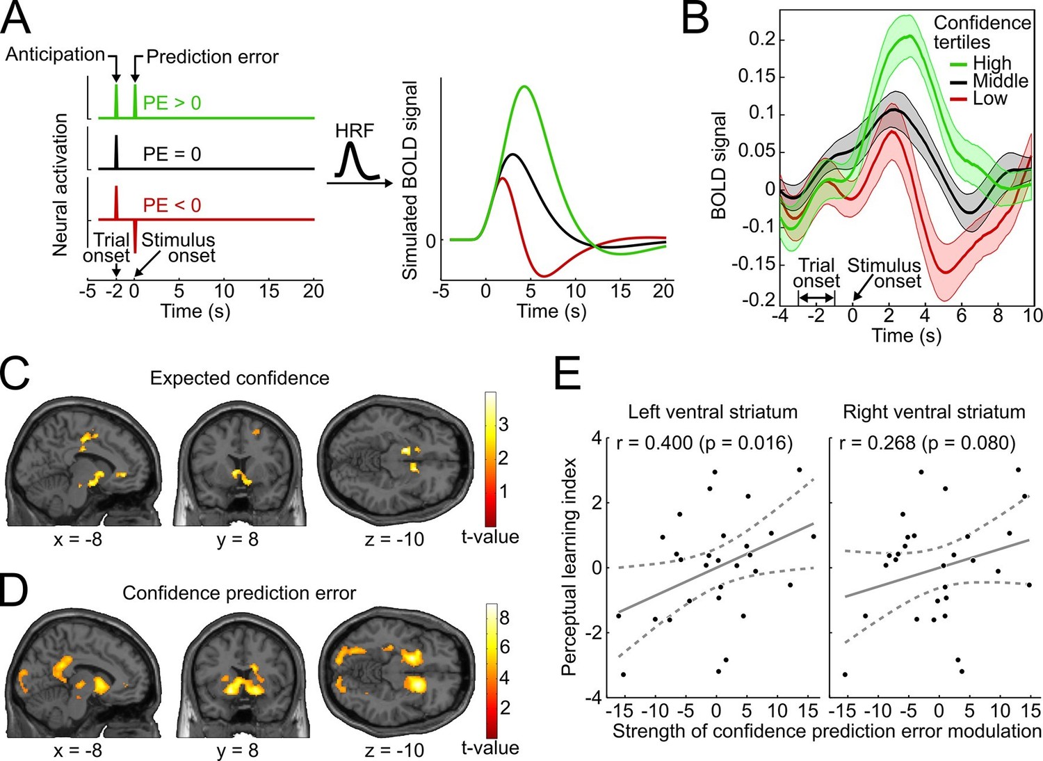
We reasoned that if confidence-based internal feedback and reward-based external feedback share a common neural basis, neural responses in the ventral striatum to high-, average- and low-confidence events should exhibit a qualitatively similar pattern as reported for rewarding, neutral and punishing outcomes in reward-based learning (Delgado et al., 2000; Knutson et al., 2001). The results of these previous studies suggest that striatal activation reflects a positive anticipatory response at the beginning of a trial as well as a subsequent prediction error response related to the outcome. To simulate the BOLD response that arises from such a scheme, we convolved vectors coding the neural activation for an initial anticipatory response and three different outcome scenarios (positive, absent and negative prediction error) with a canonical double-gamma hemodynamic response function (Figure 5A). In accordance with the fMRI results of these previous studies, the simulation shows (i) an increase of striatal BOLD responses related to trial onset reflecting the anticipatory signal, and (ii) a subsequent positive, absent, or negative deflection of the BOLD response reflecting prediction errors.

Figure 5 with 1 supplement see all

Download asset Open asset

To relate the neural signature of confidence in the present study to the simulation and to the results of previous reward-based studies, we binned the data into tertiles of the behavioral confidence rating (low, middle, and high confidence) and extracted the average BOLD time course in an anatomical mask of the ventral striatum using the SPM toolbox rfxplot (Gläscher, 2009). As shown in Figure 5B, the obtained event-related BOLD time courses are in remarkable agreement with the predictions of the simulation of Figure 5A and previous empirical findings of reward studies (Delgado et al., 2000). Specifically, 4–6 s after trial onset (reflecting the hemodynamic delay), the BOLD time courses exhibited a first peak, consistent with an anticipatory confidence signal at the start of a trial; 4–6 s after stimulus onset, the BOLD time courses displayed a positive deflection for high-confidence trials and a negative deflection for low-confidence trials. A statistical analysis confirmed above-baseline striatal activation at trial onset, indicative of an anticipatory signal (left peak at [−10 14 −6], t₂₈ = 6.42, p_rFWE < 0.001; right peak at [12 14 −8], t₂₈ = 7.78, p_rFWE < 0.001), as well as a main effect of confidence at stimulus onset in the bilateral ventral striatum (left peak at [−10 14 −4], t₂₈ = 10.56, p_rFWE < 0.001; right peak at [16 12 −8], t₂₈ = 11.46, p_rFWE < 0.001). This model-free assessment provides initial support for the idea that reinforcement based on reward and based on confidence share a common neural substrate both in the anticipation and the outcome period. In addition, the results lend plausibility to a model utilizing confidence as a reinforcement signal.

Model-based analysis of brain activation

Expected confidence

To link the confidence-based reinforcement learning model to brain activity, we estimated a new general linear model (GLM) using two time-varying parametric variables generated from the model: expected confidence at trial onset and CPE at stimulus onset. As conjectured, we found a significant parametric modulation of striatal activation by expected confidence at trial onset (right peak at [8 14 −4], t₂₈ = 4.12, p_rFWE = 0.018; left peak at [−12 20 −2], t₂₈ = 3.97, p_rFWE = 0.026; Figure 5C). This model-based result corroborates the notion that striatal activation at trial onset reflects anticipated confidence for the upcoming stimulus presentation, analogous to previous findings of an anticipatory reward signal in the ventral striatum (Delgado et al., 2000; Preuschoff et al., 2006; Knutson et al., 2001).

Confidence prediction error

Using the parametric CPE regressor, we next tested for a positive linear relationship between BOLD and the CPE at the time of stimulus presentation (Figure 5D). As hypothesized, the bilateral ventral striatum showed a strong positive relationship with the CPE (left peak at [−16 8 −10], t₂₈ = 7.64, p_rFWE < 0.001; right peak at [16 14 −8], t₂₈ = 7.81, p_rFWE < 0.001). This modulation was also present in our second region of interest, the ventral tegmental area (peak at [−6 −22 −16], t₂₈ = 3.02, p_rFWE=0.027; see Supplementary file 2 for a whole-brain list of active brain regions). A complementary analysis ruled out that this modulation was due to stimulus salience (Figure 5—figure supplement 1). In sum, the CPE was represented by the same key brain structures that have been implicated in signaling reward prediction errors (Schultz et al., 1997; O’Doherty et al., 2004; Berns et al., 2001).

Orientation energy and decision value

To assess whether the model variables associated with the sensory and decisional subsystem would be reflected in brain activity, we performed a multivariate whole-brain searchlight (Kriegeskorte et al., 2006) analysis using cross-validated MANOVA (Allefeld and Haynes, 2014). As a variable describing the sensory evidence, we used orientation energy (OE), defined as the sign of the stimulus orientation (ccw = −1, cw = 1) in conjunction with the corresponding orientation energy tertile (low = 0.5, middle = 1.5, high = 2.5). We then searched for brain areas showing a multivariate linear relationship with OE. We found that OE was encoded in left occipital cortex (peak at [−44 70 0], t₂₈ = 4.77, p_cFWE = 0.033), an area overlapping with voxels activated by the stimulus localizer (Figure 6A). An additional ROI analysis to track the distinctness of stimulus-coding patterns across training runs within the control condition (constant contrast) was not feasible due to a lack of statistical power, i.e., decoding of orientation energy within a localizer-based visual cortex ROI was not possible when the data were restricted to the constant contrast condition (mean pattern distinctness ± SEM, D = 0.0029 ± 0.0033, t₂₈ = 0.86, p = 0.198, one-tailed t-test against the null hypothesis of a pattern distinctness equal to zero).

Figure 6

Download asset Open asset

For the analysis of the decision value (DV), trials were sorted in an analogous manner, such that negative and positive DVs (reflecting the model’s tendency for counterclockwise and clockwise choices) were separately sorted into DV tertiles. Interestingly, decoding of DV showed only a trend in sensory occipital cortices (peak at [−40 −72 26], t₂₈ = 3.35, p = 0.001, uncorrected). Instead, we found significant encoding of the DV in right middle frontal gyrus (peak at [32 14 44], t₂₈ = 5.87, p_FWE = 0.026; Figure 6B), in line with a recent report (Hebart et al., 2014). Thus, perceptual and decision variables of our model can be mapped to visual and frontal cortex, respectively.

In this study, we used perceptual learning to address the question of how humans can improve performance in the absence of external feedback. Previous reinforcement learning accounts of perceptual learning were based on external cognitive and rewarding feedback (Law and Gold, 2009; Kahnt et al., 2011) and could not explain the established phenomenon of perceptual learning without such feedback (Herzog and Fahle, 1997; Gibson and Gibson, 1955; McKee and Westheimer, 1978; Karni and Sagi, 1991). Here, we suggest that observers are capable of generating internal feedback by utilizing confidence signals that provide a graded evaluation of the correctness of a perceptual decision. In this way, confidence may serve as a reinforcement signal similar to reward and guide perceptual learning in cases where no external feedback is provided.

In support of this view, our model-free fMRI analyses revealed that mesolimbic confidence signals mirror those typically found for reward, both in the anticipation period (Preuschoff et al., 2006; Delgado et al., 2000; Knutson et al., 2001) and for prediction errors (Schultz et al., 1997; O’Doherty et al., 2004; Berns et al., 2001). To establish a mechanistic ground for this suggested parallel, we devised an associate reinforcement learning model, which links behavior to computational variables that each account for a different aspect of the learning process. CPEs served as feedback in the model, defined as the difference between the current level of confidence and a long-term estimate of expected confidence. The model successfully described the learning process as a continuous adjustment of a perceptual filter linking sensory and decision units. Our model-based fMRI analyses confirmed and extended the results of the model-free analyses by demonstrating a parametric modulation in mesolimbic brain areas both by expected confidence and confidence prediction. Importantly, the strength of the striatal modulation by CPEs predicted participants’ perceptual improvements, further corroborating the behavioral relevance of these internally-generated feedback signals.

The observed pattern of confidence-related activity in the mesolimbic system, including the co-modulation of the ventral tegmental area, fit well with the prediction error hypothesis of dopamine, which posits that dopaminergic midbrain neurons and their targets respond at two time points during a learning trial (Schultz et al., 1997). In this framework, the first response is triggered by an outcome-predictive cue and reflects an anticipatory signal. In the case of classical reinforcement learning, such a cue may be probabilistically coupled with rewards of possibly varying magnitudes. The anticipated value of the cue is then assumed to be computed as the average reward magnitude—contingent on the cue—in previous trials (Schultz, 2006). Here, we argue that the same principle could hold for confidence: participants learn to anticipate a certain level of confidence for the upcoming trial based on past confidence experiences, and this anticipatory state is activated when the beginning of a new trial is indicated (equivalent to a cue). In congruence with this postulation, we indeed found a modulation of striatal activity by expected confidence at trial onsets—as previously reported for expected reward (Preuschoff et al., 2006; Delgado et al., 2000; Knutson et al., 2001). The second response is triggered by the actual outcome and corresponds to a prediction error signal. In classical reinforcement learning, the reward prediction error represents the difference between expected value and actual outcome. In the confidence domain, the outcome would correspond to the level of confidence calculated from the stimulus and the prediction error would be computed as the difference between expected confidence and actual confidence. Overall, our results may therefore indicate that self-generated confidence assumes the role of external reward in dopaminergic prediction-error-based reinforcement learning when no external feedback is available.

A number of previous studies have used reinforcement learning models to capture the neural underpinnings of perceptual learning (Law and Gold, 2009; Kahnt et al., 2011) and category learning (Daniel and Pollmann, 2012). In particular, an fMRI study by Kahnt and colleagues (Kahnt et al., 2011) investigated perceptual learning with external reward and found that behavioral improvements were well explained by a reinforcement learning model. Their results exhibit a notable parallel to the present findings: the authors reported stimulus information encoded in visual cortex and model-derived decision value in frontal cortices, in agreement with the findings of the present study. In addition, this previous study identified a perceptual learning-related reward prediction error in the ventral striatum, dovetailing with our finding of a perceptual learning-related confidence prediction error in the same brain region. Importantly, our combined Hebbian and reinforcement learning model extends and improves previous models in several ways. First and foremost, by implementing confidence prediction errors in replacement of reward prediction errors, it extends previous reward reinforcement learning models of perceptual learning (Law and Gold, 2009; Kahnt et al., 2011) to cases without feedback. Second, these previous models were based on the assumption that perceptual performance is determined by a single 'readout weight', representing the amplification of stimulus information in sensory areas. While the simplicity of these models is appealing, they are limited in the sense that negative prediction errors have an unreasonable influence on behavior: according to these models, worse-than-expected feedback reduces the readout weight, which leads to an additional reduction in performance. This property runs counter to the idea that reinforcement learning agents improve their behavior through both positive and negative prediction errors. By contrast, the associative reinforcement learning rule of the present model entails a behaviorally advantageous and plausible function of negative prediction errors: inhibition of sensory noise. Third, a conceptually related reinforcement learning model for perceptual categorization (Daniel and Pollmann, 2012) implies that stimuli exclusively activate the correct stimulus category, an assumption that disregards the fact that the ambiguity of incoming stimulus information is an essential property of perceptually demanding tasks. In contrast, the present model utilizes a dedicated representational subsystem (Petrov et al., 2005) to estimate the activation of all implemented input units, and it is their differential activity that determines perceptual choices.

The present model and results are biologically plausible and fit well with theoretical accounts of the neural basis of learning. The associative reinforcement learning rule in the model was inspired by the three-factor learning rule (Schultz, 2002; Reynolds et al., 2001), which has been proposed to underlie the potentiation of synapses in the striatum. It proposes that changes in neural transmission in cortico-striatal synapses not only depend on coincident presynaptic and postsynaptic activity (Hebbian learning), but also on the presence of dopamine error signals. Indeed, Ashby and colleagues (Ashby et al., 2007; Hélie et al., 2015) have previously suggested that the basal ganglia, which represent the predominant site of dopaminergic synaptic plasticity, are themselves a key region for learning in perceptual tasks. They proposed that (i) the basal ganglia serve to activate the appropriate target regions in executive frontal cortices shortly after sensory cortex activation; and (ii) such basal ganglia learning is superseded by cortico-cortical Hebbian learning, once the correct cortico-cortical synapses are built. This account fits well with the present model, in which perceptual learning corresponds to the process of reweighting connections between sensory and decisional units. These considerations in combination with the present results thus lend support to the hypothesis that the optimization of perceptual read-out (as implicated by our model) could be mediated via reinforcement learning in the basal ganglia.

While our study represents a first but important step towards understanding the role of confidence signals in perceptual learning, future studies are needed to investigate in more detail the characteristics of these signals which were not addressed in the current study. First, are these signals triggered independent of whether participants have to report their level of confidence after the percept or independent of whether they receive external feedback? Investigating these questions could clarify whether the observed activity in the reward network is an automatic response or depends on the task of the observer. Second, are these learning signals independent of making a perceptual decision? In other words, are they triggered only when participants have to engage in a subsequent perceptual choice? Similarly, can these confidence signals be disentangled from choice accuracy, for instance by manipulating stimulus luminance (Busey et al., 2000)? An answer to this latter question would shed light on the nature of the confidence signals, i.e. whether they can also be affected by metacognitive biases.

In summary, our study devised and tested a novel model of perceptual learning in the absence of external feedback, utilizing confidence prediction errors to guide the learning process. Our analyses revealed a compelling analogy between confidence-based and reward-based feedback, suggesting a similar neural mechanism for learning with and without external feedback. Future work could investigate whether a learning mechanism based on such self-generated feedback is also applicable outside the realm of perception, where learning without feedback has likewise been a long-standing puzzle (Köhler, 1925).

1. 1. Allefeld C
   2. Haynes JD

   (2014) Searchlight-based multi-voxel pattern analysis of fMRI by cross-validated MANOVA

   NeuroImage 89:345–357.

   https://doi.org/10.1016/j.neuroimage.2013.11.043

   • Google Scholar
2. 1. Ashby FG
   2. Ennis JM
   3. Spiering BJ

   (2007) A neurobiological theory of automaticity in perceptual categorization

   Psychological Review 114:632–656.

   https://doi.org/10.1037/0033-295X.114.3.632

   • Google Scholar
3. 1. Barto AG
   2. Sutton RS
   3. Brouwer PS

   (1981) Associative search network: A reinforcement learning associative memory

   Biological Cybernetics 40:201–211.

   https://doi.org/10.1007/BF00453370

   • Google Scholar
4. 1. Berns GS
   2. McClure SM
   3. Pagnoni G
   4. Montague PR

   (2001)

   Predictability modulates human brain response to reward

   Journal of Neuroscience 21:2793–2798.

   • Google Scholar
5. 1. Busey TA
   2. Tunnicliff J
   3. Loftus GR
   4. Loftus EF

   (2000) Accounts of the confidence-accuracy relation in recognition memory

   Psychonomic Bulletin & Review 7:26–48.

   https://doi.org/10.3758/BF03210724

   • Google Scholar
6. 1. Cousineau D

   (2005)

   Confidence intervals in within-subject designs: A simpler solution to Loftus and Masson’s method

   Tutorial in Quantitative Methods for Psychology 1:42–45.

   • Google Scholar
7. 1. Daniel R
   2. Pollmann S

   (2012) Striatal activations signal prediction errors on confidence in the absence of external feedback

   NeuroImage 59:3457–3467.

   https://doi.org/10.1016/j.neuroimage.2011.11.058

   • Google Scholar
8. 1. Delgado MR
   2. Nystrom LE
   3. Fissell C
   4. Noll DC
   5. Fiez JA

   (2000)

   Tracking the hemodynamic responses to reward and punishment in the striatum

   Journal of Neurophysiology 84:3072–3077.

   • Google Scholar
9. 1. Duijvenvoorde AC
   2. Op de Macks ZA
   3. Overgaauw S
   4. Gunther Moor B
   5. Dahl RE
   6. Crone EA

   (2014) A cross-sectional and longitudinal analysis of reward-related brain activation: effects of age, pubertal stage, and reward sensitivity

   Brain and Cognition 89:3–14.

   https://doi.org/10.1016/j.bandc.2013.10.005

   • Google Scholar
10. 1. Garcı́a-Pérez MA

    (1998) Forced-choice staircases with fixed step sizes: asymptotic and small-sample properties

    Vision Research 38:1861–1881.

    https://doi.org/10.1016/S0042-6989(97)00340-4

    • Google Scholar
11. 1. Gibson EJ

    (1963) Perceptual learning

    Annual Review of Psychology 14:29–56.

    https://doi.org/10.1146/annurev.ps.14.020163.000333

    • Google Scholar
12. 1. Gibson JJ
    2. Gibson EJ

    (1955) Perceptual learning; differentiation or enrichment?

    Psychological Review 62:32–41.

    https://doi.org/10.1037/h0048826

    • Google Scholar
13. 1. Gläscher J

    (2009) Visualization of group inference data in functional neuroimaging

    Neuroinformatics 7:73–82.

    https://doi.org/10.1007/s12021-008-9042-x

    • Google Scholar
14. 1. Hebart MN
    2. Schriever Y
    3. Donner TH
    4. Haynes JD

    (2016) The Relationship between Perceptual Decision Variables and Confidence in the Human Brain

    Cerebral Cortex 26:.

    https://doi.org/10.1093/cercor/bhu181

    • Google Scholar
15. 1. Herzog MH
    2. Fahle M

    (1997) The role of feedback in learning a vernier discrimination task

    Vision Research 37:2133–2141.

    https://doi.org/10.1016/S0042-6989(97)00043-6

    • Google Scholar
16. Book

    1. Hulley S
    2. Cummings S
    3. Browner W
    4. Grady D
    5. Newman T

    (2013)

    Designing clinical research: an epidemiologic approach (4th eds)

    Philadelphia, PA: Lippincott Williams & Wilkins.

    • Google Scholar
17. 1. Hélie S
    2. Ell SW
    3. Ashby FG

    (2015) Learning robust cortico-cortical associations with the basal ganglia: An integrative review

    Cortex 64:123–135.

    https://doi.org/10.1016/j.cortex.2014.10.011

    • Google Scholar
18. 1. Jaušovec N
    2. Jaušovec K

    (2010) Resting brain activity: differences between genders

    Neuropsychologia 48:3918–3925.

    https://doi.org/10.1016/j.neuropsychologia.2010.09.020

    • Google Scholar
19. 1. Kaernbach C

    (1991) Simple adaptive testing with the weighted up-down method

    Perception & Psychophysics 49:227–229.

    https://doi.org/10.3758/BF03214307

    • Google Scholar
20. 1. Kahnt T
    2. Grueschow M
    3. Speck O
    4. Haynes JD

    (2011) Perceptual learning and decision-making in human medial frontal cortex

    Neuron 70:549–559.

    https://doi.org/10.1016/j.neuron.2011.02.054

    • Google Scholar
21. 1. Karni A
    2. Sagi D

    (1991) Where practice makes perfect in texture discrimination: evidence for primary visual cortex plasticity

    Proceedings of the National Academy of Sciences of the United States of America 88:4966–4970.

    https://doi.org/10.1073/pnas.88.11.4966

    • Google Scholar
22. 1. Karni A
    2. Sagi D

    (1993) The time course of learning a visual skill

    Nature 365:250–252.

    https://doi.org/10.1038/365250a0

    • Google Scholar
23. 1. Knutson B
    2. Adams CM
    3. Fong GW
    4. Hommer D

    (2001)

    Anticipation of increasing monetary reward selectively recruits nucleus accumbens

    Journal of Neuroscience 21:RC159.

    • Google Scholar
24. 1. Kriegeskorte N
    2. Goebel R
    3. Bandettini P

    (2006) Information-based functional brain mapping

    Proceedings of the National Academy of Sciences of the United States of America 103:3863–3868.

    https://doi.org/10.1073/pnas.0600244103

    • Google Scholar
25. 1. Kvam PD
    2. Pleskac TJ
    3. Yu S
    4. Busemeyer JR

    (2015) Interference effects of choice on confidence: Quantum characteristics of evidence accumulation

    Proceedings of the National Academy of Sciences 112:10645–10650.

    https://doi.org/10.1073/pnas.1500688112

    • Google Scholar
26. Book

    1. Köhler W

    (1925)

    The Mentality of Apes

    New York, NY: Liveright.

    • Google Scholar
27. 1. Law CT
    2. Gold JI

    (2009) Reinforcement learning can account for associative and perceptual learning on a visual-decision task

    Nature Neuroscience 12:655–663.

    https://doi.org/10.1038/nn.2304

    • Google Scholar
28. 1. Mckee SP
    2. Westhe G

    (1978) Improvement in vernier acuity with practice

    Perception & Psychophysics 24:258–262.

    https://doi.org/10.3758/BF03206097

    • Google Scholar
29. 1. O'Doherty J
    2. Dayan P
    3. Schultz J
    4. Deichmann R
    5. Friston KJ
    6. Dolan RJ

    (2004) Dissociable Roles of Ventral and Dorsal Striatum in Instrumental Conditioning

    Science 304:452–454.

    https://doi.org/10.1126/science.1094285

    • Google Scholar
30. 1. Petrov AA
    2. Dosher BA
    3. Lu ZL

    (2005) The dynamics of perceptual learning: an incremental reweighting model

    Psychological Review 112:715–743.

    https://doi.org/10.1037/0033-295X.112.4.715

    • Google Scholar
31. 1. Petrov AA
    2. Dosher BA
    3. Lu ZL

    (2006) Perceptual learning without feedback in non-stationary contexts: data and model

    Vision Research 46:3177–3197.

    https://doi.org/10.1016/j.visres.2006.03.022

    • Google Scholar
32. 1. Preuschoff K
    2. Bossaerts P
    3. Quartz SR

    (2006) Neural differentiation of expected reward and risk in human subcortical structures

    Neuron 51:381–390.

    https://doi.org/10.1016/j.neuron.2006.06.024

    • Google Scholar
33. 1. Reynolds JN
    2. Hyland BI
    3. Wickens JR

    (2001) A cellular mechanism of reward-related learning

    Nature 413:67–70.

    https://doi.org/10.1038/35092560

    • Google Scholar
34. 1. Ruigrok AN
    2. Salimi-Khorshidi G
    3. Lai MC
    4. Baron-Cohen S
    5. Lombardo MV
    6. Tait RJ
    7. Suckling J

    (2014) A meta-analysis of sex differences in human brain structure

    Neuroscience and Biobehavioral Reviews 39:34–50.

    https://doi.org/10.1016/j.neubiorev.2013.12.004

    • Google Scholar
35. 1. Schlagenhauf F
    2. Rapp MA
    3. Huys QJ
    4. Beck A
    5. Wüstenberg T
    6. Deserno L
    7. Buchholz HG
    8. Kalbitzer J
    9. Buchert R
    10. Bauer M
    11. Kienast T
    12. Cumming P
    13. Plotkin M
    14. Kumakura Y
    15. Grace AA
    16. Dolan RJ
    17. Heinz A

    (2013) Ventral striatal prediction error signaling is associated with dopamine synthesis capacity and fluid intelligence

    Human Brain Mapping 34:1490–1499.

    https://doi.org/10.1002/hbm.22000

    • Google Scholar
36. 1. Schultz W
    2. Dayan P
    3. Montague PR

    (1997) A Neural Substrate of Prediction and Reward

    Science 275:1593–1599.

    https://doi.org/10.1126/science.275.5306.1593

    • Google Scholar
37. 1. Schultz W

    (2002) Getting Formal with Dopamine and Reward

    Neuron 36:241–263.

    https://doi.org/10.1016/S0896-6273(02)00967-4

    • Google Scholar
38. 1. Schultz W

    (2006) Behavioral theories and the neurophysiology of reward

    Annual Review of Psychology 57:87–115.

    https://doi.org/10.1146/annurev.psych.56.091103.070229

    • Google Scholar
39. 1. Schwarze U
    2. Bingel U
    3. Badre D
    4. Sommer T

    (2013) Ventral striatal activity correlates with memory confidence for old- and new-responses in a difficult recognition test

    PloS One 8:e54324.

    https://doi.org/10.1371/journal.pone.0054324

    • Google Scholar
40. 1. Sieck WR

    (2003) Effects of choice and relative frequency elicitation on overconfidence: further tests of an exemplar-retrieval model

    Journal of Behavioral Decision Making 16:127–145.

    https://doi.org/10.1002/bdm.438

    • Google Scholar
41. 1. Sniezek JA
    2. Paese PW
    3. Switzer FS

    (1990) The effect of choosing on confidence in choice

    Organizational Behavior and Human Decision Processes 46:264–282.

    https://doi.org/10.1016/0749-5978(90)90032-5

    • Google Scholar
42. Book

    1. Sutton RS
    2. Barto AG

    (1998) Reinforcement Learning: An Introduction

    Cambridge, MA: Bradford Books.

    https://doi.org/10.1109/TNN.1998.712192

    • Google Scholar
43. 1. Tafarodi RW
    2. Milne AB
    3. Smith AJ

    (1999) The Confidence of Choice: Evidence for an Augmentation Effect on Self-Perceived Performance

    Personality and Social Psychology Bulletin 25:1405–1416.

    https://doi.org/10.1177/0146167299259006

    • Google Scholar
44. 1. Tzourio-Mazoyer N
    2. Landeau B
    3. Papathanassiou D
    4. Crivello F
    5. Etard O
    6. Delcroix N
    7. Mazoyer B
    8. Joliot M

    (2002) Automated anatomical labeling of activations in SPM using a macroscopic anatomical parcellation of the MNI MRI single-subject brain

    NeuroImage 15:273–289.

    https://doi.org/10.1006/nimg.2001.0978

    • Google Scholar

Author details

1. Matthias Guggenmos

   1. Bernstein Center for Computational Neuroscience, Berlin, Germany
   2. Visual Perception Laboratory, Charité Universitätsmedizin, Berlin, Germany

   Contribution

   MG, Conception and design, Acquisition of data, Analysis and interpretation of data, Drafting or revising the article

   For correspondence

   matthias.guggenmos@charite.de

   Competing interests

   The authors declare that no competing interests exist.

   "This ORCID iD identifies the author of this article:" 0000-0002-0139-4123

2. Gregor Wilbertz

   Visual Perception Laboratory, Charité Universitätsmedizin, Berlin, Germany

   Contribution

   GW, Acquisition of data, Analysis and interpretation of data, Drafting or revising the article

   Competing interests

   The authors declare that no competing interests exist.

3. Martin N Hebart

   Department of Systems Neuroscience, Universitätsklinikum Hamburg-Eppendorf, Hamburg, Germany

   Contribution

   MNH, Conception and design, Analysis and interpretation of data, Drafting or revising the article

   Contributed equally with

   Philipp Sterzer

   Competing interests

   The authors declare that no competing interests exist.

4. Philipp Sterzer

   1. Bernstein Center for Computational Neuroscience, Berlin, Germany
   2. Visual Perception Laboratory, Charité Universitätsmedizin, Berlin, Germany

   Contribution

   PS, Conception and design, Analysis and interpretation of data, Drafting or revising the article

   Contributed equally with

   Martin N Hebart

   Competing interests

   The authors declare that no competing interests exist.

• 3,677

  views

• 648

  downloads

• 82

  citations

Views, downloads and citations are aggregated across all versions of this paper published by eLife.