

Abstract
In the central visual pathway of binocular animals, the property of directional selectivity (DS) is first exhibited in striate cortex. In this study, we sought to determine the neural circuitry underlying the transformation from non-DS neurons to DS cortical cells. In a well established model, DS receptive fields (RFs) are derived from the sum of two non-DS inputs with 90° (quadrature) spatiotemporal phase differences. We explored possible input sources for this model, which include non-DS simple cells and lateral geniculate nucleus (LGN) neurons, by examination of spatiotemporal RFs of single cells and of pairs of cells. We find that distributions of non-DS simple RFs do not match the temporal predictions of the quadrature model because of a lack of long-latency responses. The long-latency inputs could potentially arise from lagged LGN afferents. However, analysis of cell pairs indicates that DS cells receive cortical input from non-DS simple cells for both short- and long-latency components, with temporal phase differences typically <90°. Furthermore, the distribution of minimum phase differences needed to generate DS cells overlaps that exhibited by non-DS simple cells. Considered together, these results are consistent with a linear model whereby DS simple cells are formed from simple-cell inputs, with temporal phase differences often less than quadrature.
Introduction
Determination of the direction of stimulus motion is a fundamental encoding requirement of the visual system. This is accomplished by retinal ganglion cells in animals with minimal binocular field overlap (Barlow and Levick, 1965; Borg-Graham, 2001; Taylor and Vaney, 2003). In species with frontally positioned eyes, directional selectivity (DS) is a cortical function (Hubel and Wiesel, 1962). A central question of visual processing concerns the determination of how non-DS input generates DS simple cells in the striate cortex. To address this question, it is useful to consider the energy model (Adelson and Bergen, 1985; Watson and Ahumada, 1985), which provides a basis for the derivation of direction selectivity. According to this theoretical construct, a pair of input filters with quadrature spatial and temporal phase differences can generate a DS receptive field (RF). This model has been used effectively in previous work (DeAngelis et al., 1993; Jagadeesh et al., 1997; De Valois and Cottaris, 1998; De Valois et al., 2000). For the current purpose, it is necessary to consider what inputs are physiologically plausible.
A recent examination of RFs in the monkey visual cortex (De Valois and Cottaris, 1998; De Valois et al., 2000) suggests the existence of two subpopulations of non-DS simple cells with the appropriate phase relationships to serve as inputs for the quadrature model. One population exhibits biphasic temporal response profiles with a short-latency onset (early phase), and the other has monophasic responses with longer latencies (late phase). However, subpopulations of simple cells with this quadrature relationship do not appear to be present in the cat because of a lack of neurons with the appropriate late-phase response profiles (Dean and Tolhurst, 1986; DeAngelis et al., 1999; Nishimoto et al., 2001). Some studies have proposed that DS simple cells in the cat receive late-phase inputs directly from lagged lateral geniculate nucleus (LGN) afferents, either in combination with other LGN cells (Saul and Humphrey, 1990) or with non-DS simple cells (Nishimoto et al., 2001).
Simple cells exhibit a broad distribution of selectivity to direction (Schiller et al., 1976; Hamilton et al., 1989; Gizzi et al., 1990; De Valois et al., 2000). In the quadrature model, different degrees of selectivity are generated by weighted sums of the input components. Strongly and weakly selective units are created by balanced and unbalanced weights, respectively. In an alternative scheme, which we refer to as the “variable phase model,” different degrees of selectivity are obtained by summation with balanced weights and phase differences in the range of 0–90°.
In the study reported here, we assess the roles of non-DS simple cells and LGN input in the generation of DS simple cells in area 17 of the cat. We determined the temporal input requirements of a large sample of DS cells according to the quadrature and variable phase models and compare these requirements with the temporal characteristics of non-DS simple and LGN RFs. More direct evaluations of intracortical connections are made by analysis of RFs of pairs of simultaneously recorded simple cells. Our results are consistent with a variable phase model with simple-cell inputs.
Materials and Methods
Extracellular recordings are made from cells in area 17 and LGN of anesthetized (sodium thiamylal or thiopental administered at a rate determined individually for each animal) and paralyzed (gallamine triethiodide, 10 mg · kg–1 · hr–1, or pancuronium, 0.1–0.2 mg · kg–1 · hr–1) adult cats. All procedures were conducted in conformance with the guidelines regarding the care and use of animals adopted by the Society for Neuroscience and according to local campus regulations. Single-unit recordings are obtained using multiple (two to four) tungsten microelectrodes (Levick, 1972; or commercial models) with impedances between 2 and 10 MΩ. For area 17 recordings, electrode penetrations are made down the medial bank of the postlateral gyrus at P4 L2.5 in Horsley-Clarke (H-C) coordinates (Horsley and Clarke, 1908) angled 10° medial and 20° anterior. Vertical electrode penetrations are made for LGN recordings at H-C coordinates A6 L9. After a unit is identified by its response waveform, RF parameters are measured using drifting sinusoidal gratings and random-noise stimuli. Details of the surgical and experimental procedures have been described previously (Cai et al., 1997; Anzai et al., 1999).
Cell classification. Cortical cells are classified as simple or complex by classical criteria (Hubel and Wiesel, 1962) and by comparing the first harmonic (F1) to the DC (F0) of the peristimulus time histogram (PSTH) to a grating drifting at 2 Hz with optimized spatial frequency and orientation. Cells with an F1/F0 ratio ≥1 are classified as simple (Skottun et al., 1991) (for an alternative view of this classification system, see Mechler and Ringach, 2002). In the LGN, X and Y cells exhibit similar linear RF organization (Cai et al., 1997), and we have not differentiated them in this study. W cells located in the C laminas (Cleland et al., 1976; Wilson et al., 1976) have been avoided. LGN cells are classified as lagged or nonlagged (Mastronarde, 1987; Saul and Humphrey, 1990) on the basis of the absolute value of the ratio of the first to second peak amplitudes of the temporal profile of the RF center. Values <1 are classified as lagged, otherwise nonlagged (Cai et al., 1997; Wolfe and Palmer, 1998). Spatiotemporal RFs are measured using a reverse correlation method (see below). This classification system is simpler than the set of tests delineated by Mastronarde (1987) and is similar to the rebound index used by Alonso et al. (2001).
Grating measurements. Spatial and temporal tuning parameters are measured using drifting sinusoidal gratings. Gratings are presented monocularly at 50% Michelson contrast with a mean luminance of 17 cd/m2. For orientation, direction selectivity, spatial frequency, and size tuning measurements, gratings are drifted at a temporal frequency of 2 Hz with other nonvariable parameters optimized for the cell. For temporal frequency tuning measurements, optimal size, spatial frequency, and orientation parameters are used. For direction selectivity measurements, the F1 amplitude of the PSTH is obtained in response to the preferred (P) and nonpreferred (NP) directions to calculate a direction selectivity index (DSI):  (1) RF measurements. Estimates of linear spatiotemporal RFs are measured using a reverse correlation procedure (Jones and Palmer, 1987; Freeman and Ohzawa, 1990). For most cells, a spatially one-dimensional space–time RF is obtained using long bars oriented along the preferred orientation of the cell. For a subpopulation of cells, a more time consuming two-dimensional RF is measured. For in-depth descriptions of the reverse correlation procedures as used here, see DeAngelis et al. (1993). Briefly, individual bar stimuli of either moderate (32 cd/m2) or low (2 cd/m2) luminance are displayed one at a time on random grid locations for 40 msec durations with a mean background luminance of 17 cd/m2. By cross-correlating the stimulus with the response, a linear approximation to the space–time RF is obtained. Before spatial and temporal parameters are computed, the RF is first interpolated using a cubic spline.
Predicted direction selectivity. The direction selectivity predicted from the linear space–time RF is determined by calculating the spatiotemporal amplitude spectrum by Fourier analysis. The predicted responses to a grating drifting in the preferred and nonpreferred directions at a given spatial frequency and 2 Hz temporal frequency are obtained by finding the values of the amplitude spectrum at that spatial frequency for +2 and –2 Hz temporal frequencies, respectively (DeAngelis et al., 1993). A DSI value is computed from the predicted responses using Equation 1.
Receptive field fitting. Spatiotemporal RFs, R(x,t), are fit using a sum of two space–time separable components:  (2) where G(x)H(t) and G′(x)H′(t) are the two components. Here, we model the spatial profile, G(x), as a Gabor function (Gabor, 1946):
  (3) which provides a good fit for simple-cell RFs (Field and Tolhurst, 1986; Jones and Palmer, 1987; DeAngelis et al., 1993). In general, the temporal profile, H(t), is not as well described by a pure Gabor function. The typical temporal response of a simple cell exhibits a rapid onset and a gradual offset and is better fit by a sigmoidally skewed Gabor function (DeAngelis et al., 1999):
  (4)
(4)  (5)
(5)  (6) where T(t) is the temporal skewing function.
The second separable component, G′(x)H′(t), is modeled with the same parameters as the first but with phase offsets in both space,  (7) and time,
  (8)
(8)  (9) For a quadrature fit to a DS (i.e., space–time inseparable) RF, the special and temporal offsets (Δφx and Δφt) are both fixed at 90°. Different levels of direction selectivity are obtained by summing the two components with different relative amplitudes:
  (10) where the resulting RFs vary from non-DS to maximally DS as α varies from 0 to 1. The k parameter scales the overall amplitude.
For a variable phase fit, different degrees of direction selectivity are obtained by summing the two components with equal amplitudes (i.e., α = 1) and allowing Δφx and Δφt to vary:  (11) The actual resulting temporal phase difference between the two components is a function of, but not always equal to, Δφt. The inequality is a result of the Gaussian envelope and temporal skew. For this reason, reported phase differences are determined by Fourier analysis, in which the characteristic phase of each component is defined at the peak temporal frequency for the inseparable RF.
Cell pair analysis. We record simultaneously a pair of RFs from potentially connected simple cells, in which one is DS and the other non-DS. We define “potentially connected” as having overlapping spatial RFs (>50% overlap) with similar orientation and spatial frequency preferences. Such pairs of cells have a high probability of being functionally connected (Ghose et al., 1994). More direct estimates of the underlying neural connections are obtained by cross-correlation (see below). However, because of the difficulties in interpreting cross-correlation histograms (CCHs) (Brody, 1998, 1999), especially with relatively low neural response rates, the classification of potentially connected is not dependent on this analysis. Here we assume that the non-DS cell of each potentially connected pair forms one of the input components to the DS cell. This allows us to infer properties of the missing input component. To estimate the shape of the RF of the missing component, we first fit the measured DS and non-DS RFs with inseparable (variable α) and separable (α = 0) versions of the quadrature fitting function (Eq. 10), respectively. Then the “missing component” is obtained by fitting the difference of the pair of RF fits with a separable function (α = 0; Eq. 10). To be included in the pairs analysis, the sum of the missing component and the non-DS RF must account for at least 66% of the variance of the DS RF.
An estimate of the synaptic connectivity between two simultaneously recorded cells is obtained via averaged cross-correlation of spiking responses across multiple visual stimulus presentations. Artifacts in the resulting CCH attributable to stimulus correlations are corrected by a shuffled subtraction technique (Perkel et al., 1967). The type of functional connectivity between the two cells is inferred from the shape of the corrected CCH (Gerstein and Perkel, 1969; Toyama et al., 1981; Ghose et al., 1994; Menz and Freeman, 2004). Here we define a sharp peak in the CCH (width <1 msec) displaced from zero by <3 msec as evidence of a monosynaptic excitatory connection. Broad peaks centered at zero are classified as common input.
Results
Distribution of degrees of direction selectivity
We measured space–time RFs for 310 simple cells from area 17 of the cat. We divided this sample into DS and non-DS units on the basis of the DSI of the cell determined both with drifting gratings and from RF analysis. The distribution of DSI values measured with drifting gratings is shown in Figure 1 (open circles). A value of 0.5 provides a good division between cells with RFs that appear separable and those that seem inseparable by visual inspection. However, a small number of cells with DSIs >0.5 exhibited space–time RFs that appeared separable. Because of this, the DSI predicted from the space–time RF was also taken into account when classifying a cell as DS. Figure 1 also shows the distribution of DSI values predicted from the linear RF (open triangles). This distribution is similar to that obtained from membrane potential recordings (Jagadeesh et al., 1997). The difference in the shape of the distribution arises because of nonlinearities in the transformation of membrane potentials to spiking activity, which is well modeled as a static power function with a mean exponent of 2.5 (DeAngelis et al., 1993). This expansive output nonlinearity enhances the direction selectivity measured from spiking responses, which shifts the DSI distribution to higher values. When an exponent of 2.5 is applied to the responses predicted from the linear RFs, the resulting DSI distribution (Fig. 1, filled triangles) is remarkably similar to the measured one (Fig. 1, open circles). Here we define cells as DS only when both measured and predicted (exponent, 2.5) DSI values are >0.5. Otherwise, cells are defined as non-DS. We should note that, in our sample, all cells with predicted DSIs >0.5 also had measured DSIs >0.5. Most cells in our sample (74%) are classified as DS using these criteria.

Different measurements of the distribution of DSI for a sample of simple cells (n = 310). Open circles, The distribution of DSI measured using drifting gratings. Open triangles, The distribution of DSI predicted from the linear RF. Filled triangles, The distribution of DSI predicted from the RF taking into account an expansive output nonlinearity modeled as an exponent of 2.5. In addition to having a measured DSI >0.5, cells must also have a predicted DSI >0.5 (as indicated by the vertical dashed line) to be classified as a DS cell.
Temporal requirements of the quadrature model
To estimate the temporal requirements of the quadrature model, we fit DS RFs with a quadrature-pair function (Eq. 10). We note that DS RFs tend to exhibit similar fitting components. For each cell, one of the components can be characterized by a fast biphasic temporal response and the other by a lagged monophasic temporal response. This is similar to the principal components found for DS RFs in the monkey (De Valois et al., 2000) and the cat (Nishimoto et al., 2001). The peak in the distribution of latencies for monophasic components (Fig. 2, open circles, solid line) falls approximately halfway between the latencies of the first and second peaks of biphasic components (short and long dashed lines), indicating a quadrature relationship. The second peak of the biphasic components exhibits a broader latency distribution (SD, 38) than the first (SD, 17), consistent with previous findings (De Valois et al., 2000) and partially reflecting the range of temporal frequency preferences for DS cells.

Distribution of latency-to-peak for quadrature fitting components of DS cells. The solid line shows time-to-peak latencies for monophasic fitting components (mean, 106.6 ± 25.5 msec). The short and long dashed lines show the latencies for the first (upward triangles; mean, 69.1 ± 17.3 msec) and second (downward triangles; mean, 150.0 ± 37.8 msec) peaks of the biphasic fitting components, respectively.
Temporal characteristics of non-DS simple cells
The latency distributions shown in Figure 2 represent estimates of the temporal requirements for inputs to DS cells based on the quadrature model. There are several input sources that could plausibly meet these requirements. Here, we considered direct input from LGN and from non-DS simple cells. In the monkey, there is evidence for two subpopulations of non-DS simple cells exhibiting monophasic and biphasic temporal responses, with phase differences in agreement with the quadrature model (De Valois et al., 2000). Some studies have suggested that similar subpopulations may not be present in the cat (DeAngelis et al., 1999; Nishimoto et al., 2001). To explore this, we divided non-DS cells into monophasic and biphasic subpopulations by use of an index consisting of the ratio of first to second peak amplitudes along the optimal time slice (i.e., biphasic index). Values near 1 indicate temporally biphasic responses with similar peak amplitudes, whereas those near 0 represent monophasic profiles. The distribution of biphasic indices shown in Figure 3 is similar to that found for the monkey (De Valois et al., 2000). Using the same conventions as De Valois et al. (2000), we classify cells with indices >0.5 as biphasic and those <0.3 as monophasic. The eight cells with indices between these values are unclassified and have been removed from the analysis.

Distribution of biphasic indices for non-DS simple cells. Cells with biphasic indices <0.3 are classified as monophasic. Cells with biphasic indices >0.5 are classified as biphasic.
Biphasic cells (Fig. 4, short and long dashed lines) exhibit temporal characteristics similar to the biphasic fitting components (Fig. 2, short and long dashed lines). The first and second peaks of the biphasic cells exhibit mean latencies of 65 ± 16 and 152 ± 36 msec, respectively. These latencies may be compared with 69 ± 17 and 150 ± 37 msec for the first and second peaks of the biphasic fitting components. These are consistent with other findings that suggest that biphasic simple cells exhibit the latencies expected from the early component of the quadrature model (Nishimoto et al., 2001).

Distribution of latency-to-peak for non-DS simple cells. The solid line shows time-to-peak latencies for monophasic cells (mean, 76.3 ± 14.4 msec). The short and long dashed lines show the latencies for the first (mean, 65.3 ± 15.5 msec) and second (mean, 152.8 ± 36.4 msec) peaks of biphasic cells, respectively. The latencies of monophasic cells and those of the first peak of biphasic cells primarily overlap and show only weakly significant differences (p < 0.05; t test).
As a population, monophasic simple cells exhibit only slightly longer latencies (76 ± 14 msec) (Fig. 4, solid line) than the first peak of biphasic cells (65 ± 16 msec) (Fig. 4, short dashed line) and not as much as expected by the quadrature model (107 ± 26 msec) (Fig. 2, solid line). The latency distribution of monophasic cells does not change significantly even if we narrow our definition to biphasic indices <0.2 (data not shown). This indicates that the temporal characteristics of non-DS simple cells in the cat only agree with the early component of the quadrature model, implying a possible role for direct input from lagged LGN cells (Nishimoto et al., 2001). This also suggests a possible species difference with the monkey in which population latency distributions for monophasic and biphasic simple cells form an approximately quadrature relationship (De Valois et al., 2000; Conway and Livingstone, 2003).
Temporal characteristics of LGN cells
One possibility is that the longer-latency components that feed into DS simple cells of the cat come directly from lagged LGN afferents (Saul and Humphrey, 1990; Nishimoto et al., 2001). To explore this potential mechanism, we analyzed the spatiotemporal RFs of 406 LGN cells. We recorded from 345 nonlagged and 61 lagged cells. In other words, we classified 15% of LGN cells as lagged. Other estimates of the percentage of lagged cells in the cat LGN range from <20% (Kwon et al., 1992; Alonso et al., 2001) to ∼40% (Mastronarde, 1987; Humphrey and Weller, 1988). The broad range of estimates has been attributed to differences in classification criteria and the impedance properties of recording electrodes (Saul and Humphrey, 1992). Despite a likely under sampling, the lagged cells we find appear to have the desired latency requirements for late components of the quadrature model (Fig. 5, solid line). The mean latency of lagged cells (98 ± 22 msec) is just slightly less than that of the monophasic fitting components (107 ± 25 msec), as is expected given thalamocortical conduction delays of a few milliseconds (Hawken et al., 1996). Assuming a 3 msec delay, the latencies of lagged cells are not statistically different from those of the monophasic fitting components (p > 0.05; t test). However, the latencies of the first peak of nonlagged LGN cells (49 ± 12 msec) are substantially faster than those of the biphasic fitting components (69 ± 17 msec), even after accounting for a thalamocortical time delay (p < 0.01; t test). Also note that the relationship between lagged and nonlagged latency distributions resembles more of a 180° phase difference than a quadrature relationship. In other words, the latencies of the lagged peaks fall within the latency distribution of nonlagged second peaks. A similar observation has been made previously (Alonso et al., 2001).

The distribution of peak latencies for different classes of LGN cells. The solid line shows the latency-to-peak for lagged cells (n = 61; mean, 97.5 ± 22.2 msec). Short and long dashed lines show, respectively, first (mean, 49.4 ± 12.0 msec) and second (mean, 119.8 ± 40.2 msec) peak latencies for nonlagged cells (n = 345).
On the basis of temporal requirements of the quadrature model, which we estimate from a quadrature fit to DS simple cells, a combination of biphasic simple cells and lagged LGN cells appears to provide the required circuit. However, this nonhierarchical model implies an elaborate combination whereby LGN cells serve as inputs at two sequential processing stages. We further evaluated this model by analysis of pairs of simple cells.
Cell pair analysis
To investigate the possibility that DS simple cells are derived from a combination of biphasic simple cells and lagged LGN cells, we recorded simultaneously from pairs of potentially connected simple cells, one of which was DS and the other non-DS. These cell pairs had spatially overlapping RFs with similar orientation and spatial frequency tuning properties (see Materials and Methods). An example of such a pair is shown in Figure 6. A and B show the spatiotemporal RFs of the simultaneously recorded DS and non-DS cells, respectively. Assuming that the non-DS cell represents one of the input components to the DS cell, the missing input component (in a two-component linear model) can be obtained by taking the difference of the DS and non-DS RFs. The difference RF (i.e., missing component), shown in Figure 6C, resembles a separable RF plausibly of either LGN or simple-cell origin. In this case, the missing component is slightly lagged relative to the recorded non-DS cell. Because all of our pairs are simple cells, if we find that missing components consistently have relatively long latencies, this implies that late input is derived from lagged LGN cells. However, if we find that non-DS members of cell pairs function as both early and late inputs, this would indicate that direct lagged LGN input is not necessary.

The difference between space–time RFs for a pair of potentially connected simple cells. A, The RF for the DS member of the cell pair. Solid and dashed contours represent “on” and “off” responses, respectively. B, The RF for the non-DS member of the cell pair. C, The space–time RF obtained by taking the difference of the DS and non-DS RFs. Here the difference resembles a separable (non-DS) cell, which could potentially be a simple cell, or a group of LGN cells.
We recorded from 22 pairs of potentially connected cells. Five of the pairs were removed from the analysis because of poor fits (see Materials and Methods). Of the 17 remaining pairs, three have CCHs that indicate monosynaptic input from the non-DS cell to the DS cell. Five pairs show CCHs indicative of common input. For this study, the remainder of the pairs are considered potentially connected in that there may be a connection that is not apparent from the CCH or that the non-DS cell is representative of the temporal response properties available as input to the DS cell.
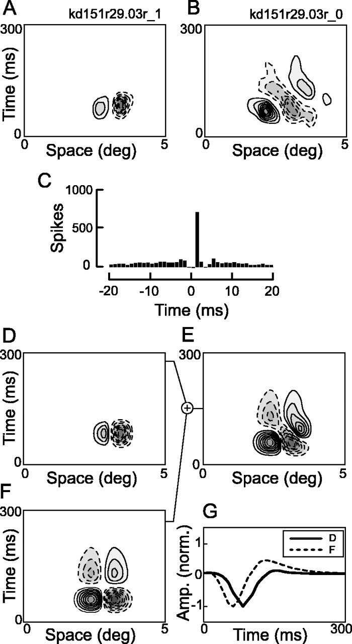
For each pair, we fit the non-DS RF with a purely separable version of the quadrature fit (α = 0; Eq. 10). We then found the best-fitting missing RF, which we also forced to be space–time separable (see Materials and Methods). A depiction of this analysis is shown in Figure 7. The recorded RFs are displayed at the top (Fig. 7A,B). The fit to the non-DS cell is shown in Figure 7D, and the best-fitting missing component in shown in Figure 7F. The sum of the non-DS RF and missing RF (Fig. 7E) produces a good fit (R2 = 0.88) to the DS RF (Fig. 7B). To compare the latencies, the temporal profiles of the non-DS and missing RFs are plotted on the same axes (Fig. 7G) as solid and dashed lines, respectively. Note that the two components are not in temporal quadrature. The missing component is only slightly phase lagged (11°) compared with the recorded non-DS cell. Nevertheless, the small temporal phase difference is enough to produce a good fit to the DS RF. Note that the CCH for this pair does not exhibit a clear functional connection (Fig. 7C).

Example pair analysis for the cells shown in Figure 6. A, B, The non-DS and DS RFs. C, The CCH of the DS and non-DS cells. This CCH does not show a clear functional connection. The horizontal axis of the CCH has been expanded to show the slow (not functionally significant) correlations. For this analysis, we assume the non-DS cell is one of two inputs to the DS cell. The analysis shown here is designed to determine the RF of the best-fitting second input. D–F, The fit to the second, i.e., missing, component (F), which when added to the fit of the non-DS RF (D), provides the best fit (E; R2 = 0.88) to the DS member of the pair (B). G, The temporal profiles of the two input RFs. Solid and dashed lines represent the temporal profiles obtained from the components in D and F, respectively. Here the temporal phase difference between the two components is only 11°.
Another example of our cell pair analysis is shown in Figure 8. In this case, the CCH indicates a monosynaptic connection from the non-DS to the DS cell (Fig. 8C). Here the missing component is in an approximate quadrature relationship with the non-DS member of the pair (Fig. 8G, temporal phase difference of –85.2°). Note that the recorded non-DS cell forms the late input. If lagged LGN afferents always supply the late input, then one would not expect to find pairs of connected simple cells such as this. This is evidence against the need for direct lagged LGN input in the derivation of direction selectivity. This argument is strengthened by the fact that the CCH of this pair indicates a monosynaptic functional connection. A second example, also with evidence of a monosynaptic connection, is shown in Figure 9. In this case, the temporal phase difference between the two input components is –46°. As in the last example, the recorded non-DS simple cell forms the late component.

Another cell pair analysis as in Figure 7. For this pair, the CCH contains a narrow peak offset from zero, which is indicative of a monosynaptic connection from the non-DS to the DS cell. Here the best-fitting missing component (R2 = 0.85) produces a temporal phase difference of –85.2°, which is approximately quadrature. The negative phase value indicates that the non-DS member of the pair functions as the late component. This is an example in which the late component is a simple cell. In other words, direct lagged input is not necessary to produce direction selectivity.

A third example of the cell pair analysis. The layout is the same as in Figure 7. As in Figure 8, this pair exhibits a CCH indicative of a monosynaptic connection from the DS to the non-DS cell. Here the best-fitting missing component (R2 = 0.74) has a temporal phase difference of –46°, indicating that the measured RF forms the late component with a relationship that is less than quadrature.
We find cell pairs with both early and late non-DS input, as indicated by the positive and negative phase differences between the recorded and missing components (Fig. 10A). This suggests that simple cells are forming both the early and the late inputs to DS cells, implying that direct input from lagged LGN cells is not necessary. Also note that the range of phase differences is more or less evenly spread between –90° and +90°. This suggests that temporal quadrature is not required to produce DS cells. These results are consistent with the variable phase model.

The distribution of temporal phase differences between the two input components. A, Phase differences determined by a fitting analysis of cell pairs (n = 17). We find both positive and negative phase differences, indicating that non-DS simple cells can form both the early and late input components of DS cells. The phase differences cover the whole range of phases from –90° to +90°, suggesting that DS cells are formed from a pair of inputs with phase differences often less than quadrature. B, A distribution of minimum temporal phase differences needed to fit DS simple cells with the same goodness of fit as for the quadrature model. The distribution is broad, suggesting that temporal quadrature is not necessary for direction selectivity.
Minimum phase fit
The distributions of latencies shown in Figure 2 are predictions based on quadrature fits to the DS RFs in our sample. For each DS RF, we determined the smallest temporal phase difference producing the same goodness of fit as the quadrature model (sequential F test; p > 0.05). The result (Fig. 10B) is a broad, and relatively flat (p > 0.5; χ2), distribution with only a small proportion (∼7%) requiring phase differences >80°. Most DS cells only require temporal phase differences <55°, suggesting that, although the non-DS latency distributions do not meet the requirements for quadrature inputs, they might be sufficient to supply the minimum phase differences needed to produce DS simple cells.
When the temporal phase difference of two input cells is <90°, there is not a clear separation between monophasic and biphasic profiles. However, if we define the component with the higher biphasic index as the biphasic component and the other as the monophasic component, we can compare the latency distributions obtained through the quadrature and variable phase models. Figure 11 shows the minimum phase latency distributions for monophasic-like (solid line) and biphasic-like (short and long dashed lines) components. Because the minimum required temporal phase differences are typically much less than 90°, the latency distribution of the more monophasic of the two components greatly overlaps the latency distribution of the first peak of the more biphasic of the components. Both are within the range of first peak latencies for non-DS simple cells (Fig. 4). This indicates that the temporal characteristics of non-DS simple cells are sufficiently diverse to generate the linear stage of DS simple cells found in the primary visual cortex of the cat.

Analysis of the minimum temporal phase necessary to fit DS cells shows a broad distribution with very few cells requiring quadrature. This figure shows the distribution of minimum phase differences in terms of latency-to-peak. Solid and dashed lines represent the distribution of peak latencies for the more monophasic (solid line; mean, 85.9 ± 34.6 msec) and more biphasic (short and long dashed lines; means, 76.6 ± 33.9 and 183.0 ± 61.1 msec, respectively) of the two components of the variable phase fit, respectively. The more monophasic component is defined as the one with the smaller biphasic index.
Considered together, these results suggest that the directionally selective responses of simple cells are derived by linear mechanisms and enhanced by static nonlinearities. The linear stage receives input from two or more non-DS simple cells with spatial and temporal phase offsets. Unlike the quadrature model, these phase offsets are not constrained to be a quarter of a cycle, and a wide range of temporal phase offsets are observed.
Discussion
We sought to determine the neural circuitry underlying the generation of DS simple cells in the primary visual cortex. We considered plausible circuits whereby the linear DS RFs are formed from the sum of non-DS inputs with spatial and temporal phase differences. The first neural circuit we considered is based on the first stage of the energy model and specifies spatial and temporal phase differences in quadrature (Adelson and Bergen, 1985; Watson and Ahumada, 1985). In this circuit, different degrees of directional selectivity are obtained by summing the inputs with different relative weights. This circuit does not adequately account for our data. Our sample of non-DS simple cells comprises mostly short to moderate latencies and lacks many RFs with a quarter-cycle temporal phase offset. This implies a possible role for direct input from lagged LGN cells; however, our analysis of pairs of simple cells reveals that non-DS simple cells can provide input for both the early- and late-phase components. This suggests that direct input from lagged LGN cells is not necessary.
The second circuit we considered combines inputs with equal weights and produces different degrees of directional selectivity by allowing the phase differences to vary. Our results are consistent with this circuit. We find that the minimum temporal phase required to form DS simple cells is typically much less than quadrature. Furthermore, the distribution of minimum phases agrees with the latency distributions of non-DS simple cells. Considered together, our results suggest that the linear RFs of DS simple cells are derived from the sum of two non-DS simple cells with temporal phase differences that are often less than quadrature. Relatively small temporal phase differences, when combined with static nonlinearities, can result in highly direction-selective response properties.
Distribution of direction selectivity
In this study, we classified 74% of simple cells in area 17 as directionally selective. This value is on the high end of the range of percentages reported for the cat. Using the same criteria (DSI >0.5), most studies report somewhere between 60 and 70% DS cells (Hamilton et al., 1989; Gizzi et al., 1990; McLean et al., 1994; Carandini and Ferster, 2000). A couple of studies suggest that fewer than 50% of simple cells are DS (Orban et al., 1981; Berman et al., 1987), and some find up to 80% (Humphrey and Saul, 1998). The relatively wide range of reported percentages can be accounted for, in part, by variations in stimulus parameters (Hammond and Pomfrett, 1990; Casanova et al., 1992) and possibly different electrode penetrations (Berman et al., 1987). The percentages reported in the cat are typically higher than in the monkey, which range from 20 to 60% (Schiller et al., 1976; De Valois et al., 1982, 2000; Albright, 1984; Hamilton et al., 1989; O'Keefe et al., 1998). Some studies in the cat find a trimodal distribution of DSI values with peaks near 0, 0.5, and 1 (Berman et al., 1987). This is similar to what is observed in the monkey (De Valois et al., 2000). However, we find a more continuous distribution of DSI values (Fig. 1). This difference in distributions, together with the relatively high percentage of DS cells, indicates that our sample might under represent non-DS cells. One possibility is that our sample lacks many long-latency non-DS simple cells just as we find relatively few lagged LGN cells. However, we have no direct evidence regarding this possibility.
Multiple derivations of directional selectivity
The results presented here suggest that direct input from lagged LGN cells is not necessary to produce the range of DS simple cells observed in area 17. We find evidence for non-DS simple cell input for both early- and late-phase components. However, this does not imply that lagged cells are not involved. Late-phase non-DS simple cells might receive mainly lagged input, and some DS cells may be generated by direct lagged input whereas others receive mainly non-DS simple cell input. Evidence that lagged cells feed into simple cells (Alonso et al., 2001) and that cooling the visual cortex does not diminish directional selectivity for at least some cells (Ferster et al., 1996) suggests that lagged cells are involved at some level. However, area 18 appears to have a higher percentage of DS cells (Orban et al., 1981; McLean et al., 1994), and it receives mainly Y LGN input (Humphrey et al., 1985), yet it is reported that Y cells are almost entirely nonlagged (Saul and Humphrey, 1990; Mastronarde et al., 1991). This raises the possibility that some DS simple cells are generated mainly by the spatial and temporal phase offsets of direct LGN afferents and that others, such as the cell pairs with monosynaptic connections reported here, and possibly area 18 cells, are generated mainly from non-DS simple cells.
The model proposed here, in which non-DS simple cells sum together to form DS simple cells, is similar to that proposed for the monkey (De Valois et al., 2000) and accounts for some, but not all, of the properties reported for DS cells. For instance, there is evidence that directional selectivity is dependent on intracortical inhibitory mechanisms (Tsumoto et al., 1979; Sillito, 1984; Livingstone, 1998). Perhaps the blockage of inhibitory mechanisms reduces directional selectivity by affecting the push–pull mechanisms of simple cells (Hubel and Wiesel, 1962; Palmer and Davis, 1981; Ferster, 1988; Hirsch et al., 1998). Another possibility is that some DS cells might be generated from the difference instead of the sum of two non-DS inputs. Theoretically, subtractive mechanisms can be as effective as additive ones in the generation of space–time inseparable RFs. Although we did not find direct evidence for inhibitory connections from non-DS to DS simple cells, these connections are difficult to detect using extracellular techniques (Aertsen and Gerstein, 1985; Melssen and Epping, 1987).
Some DS simple cells exhibit almost completely separable space–time RFs but nevertheless are DS when tested with drifting gratings. We find a small number of such cells in this study but treat them as non-DS cells for the purpose of analyzing their RFs. Other studies suggest that these cells are mostly found in layer 6 and exhibit different properties than DS simple cells found in other layers (Murthy et al., 1998). Therefore, it appears that there may be several circuits that generate DS simple cells in the visual cortex.
Comparison with findings in the primate
In recent studies of simple cells in an anesthetized monkey preparation, populations are reported of monophasic and biphasic non-DS RFs with timing characteristics that agree with a quadrature model of direction selectivity (De Valois and Cottaris, 1998; De Valois et al., 2000; Conway and Livingstone, 2003). This is interpreted as evidence for a hierarchical system in which LGN cells feed into non-DS simple cells, which in turn combine to generate DS simple cells. The data reported here, from a cat preparation, also are consistent with a hierarchical system but not necessarily with quadrature phase differences. In the cat, it appears that smaller temporal phase differences are involved, which may be accentuated by higher output nonlinearities.
Footnotes
This work was supported by National Eye Institute Research and Core Grants EY-01175 and EY-03176. We thank G. DeAngelis for helpful comments on a draft of this manuscript.
Correspondence should be addressed to Ralph D. Freeman, Group in Vision Science, School of Optometry, Helen Wills Neuroscience Institute, University of California, Berkeley, 360 Minor Hall, Berkeley, CA 94720-2020. E-mail: freeman{at}neurovision.berkeley.edu.
DOI:10.1523/JNEUROSCI.5398-03.2004
Copyright © 2004 Society for Neuroscience 0270-6474/04/243583-09$15.00/0


