

Abstract
Avian nucleus magnocellularis (NM) spikes provide a temporal code representing sound arrival times to downstream neurons that compute sound source location. NM cells act as high-pass filters by responding only to discrete synaptic events while ignoring temporally summed EPSPs. This high degree of input selectivity insures that each output spike from NM unambiguously represents inputs that contain precise temporal information. However, we lack a quantitative description of the computation performed by NM cells. A powerful model for predicting output firing rate given an arbitrary current input is given by a linear/nonlinear cascade: the stimulus is compared with a known relevant feature by linear filtering, and based on that comparison, a nonlinear function predicts the firing response. Spike-triggered covariance analysis allows us to determine a generalization of this model in which firing depends on more than one spike-triggering feature or stimulus dimension. We found two current features relevant for NM spike generation; the most important simply smooths the current on short time scales, whereas the second confers sensitivity to rapid changes. A model based on these two features captured more mutual information between current and spikes than a model based on a single feature. We used this analysis to characterize the changes in the computation brought about by pharmacological manipulation of the biophysical properties of the neurons. Blockage of low-threshold voltage-gated potassium channels selectively eliminated the requirement for the second stimulus feature, generalizing our understanding of input selectivity by NM cells. This study demonstrates the power of covariance analysis for investigating single neuron computation.
- sound localization
- covariance analysis
- phase-locking
- potassium channel
- spike
- nucleus magnocellularis
Introduction
In avians, nucleus magnocellularis (NM) is a relay hub for information from the auditory nerve used for sound localization in the azimuthal plane. NM neurons have several specializations that preserve the sub-millisecond time code present in the eighth nerve input, including a calyceal synaptic input (Jhaveri and Morest, 1982), fast receptor kinetics (Zhang and Trussell, 1994), and intrinsic membrane properties such as a large low-threshold voltage-gated potassium conductance (Reyes et al., 1994; Trussell, 1999). Preservation, and even sharpening (Joris et al., 1994), of the eighth nerve time code is essential because NM cells send their efferent signals to both ipsilateral and contralateral nucleus laminaris, which computes sound localization by acting as a coincidence detector of synaptic input arriving via delay lines from ipsilateral and contralateral sides (Jeffress, 1948; Carr and Konishi, 1990). Given the functional role of NM in the sound localization circuit, it is important to ask what computation NM neurons perform. Responses to simple stimuli such as direct current (DC) steps and phase-locked EPSC trains show that NM filters out constant current input but can reliably follow realistic high-frequency input with sub-millisecond precision (Reyes et al., 1994). This ensures the preservation of precise temporal structure while selectively filtering inputs without such structure. Although these studies provide insight into the intrinsic properties of NM cells, they are not general and are difficult to quantify.
In a Hodgkin-Huxley-style conductance-based approach, accurate dynamical models including a variety of channel types and their kinetics are used to reproduce the response of the system to simple stimuli. Here, rather than a detailed, deterministic dynamical model, we seek a functional model that provides a direct insight into the computation that the neuron performs on its inputs. By stimulating the system with a randomly varying input and correlating spiking responses with stimulus fluctuations, one can discover the features of the input that trigger spikes (Marmarelis and Marmarelis, 1978; Hunter and Korenberg, 1986). One can then build a statistical model for the probability to generate a spike in response to an arbitrary stimulus that consists of a set of features (the neural “receptive field”) and a threshold or gain function over those features (Shapley and Victor, 1978, 1979a,b, 1980; de Ruyter van Steveninck and Bialek, 1988; Berry et al., 1997; Brenner et al., 2000a; Chichilnisky, 2001). The form of these features and the gain function are determined by the biophysical properties of the neuron. In the simplest approximation, the feature is simply the spike-triggered average (STA). Covariance methods (de Ruyter van Steveninck and Bialek, 1988; Brenner et al., 2000a) allow one to determine multiple features in the stimulus that are relevant to spike generation, providing more complete descriptions of the neural feature space (Agüera y Arcas et al., 2000, 2003; Brenner et al., 2000a; Schwartz et al., 2001; Touryan et al., 2002; Fairhall et al., 2003; Petersen and Diamond, 2003; Horwitz et al., 2004; Rust et al., 2005). Although in studies of sensory responses to external stimuli it is difficult to determine the origins of neural feature selectivity in terms of biophysics or circuitry, here the system is isolated to a single neuron with current input. Thus, we combine this analysis with pharmacological manipulation of specific ion channels to understand the biophysical determinants of the feature selectivity of NM.
Materials and Methods
Slice preparation. Details of the slicing procedure are outlined in the study by Reyes et al. (1994). Briefly, chicks (embryonic days 20-21) were decapitated, and a 1.5 cm section of the skull containing the brainstem was removed with a razor blade and quickly submerged in ice-cold cutting solution containing the following (in mm): 105 choline-Cl, 5 KCl, 5 MgCl2, 26 NaHCO3, 1.25 NaH2PO4, 20 TEA-Cl, 20 sucrose, 10 dextrose, 1.3 Na-ascorbate, and 2.4 pyruvic acid. An 80 mm transverse section of the brainstem containing NM was dissected and transferred to a Vibratome tissue slicer (TPI, St. Louis, MO). Approximately six 200 μm coronal slices were made and placed in separate compartments in a holding chamber filled with artificial CSF (ACSF), incubated at 34°C for 30 min, and cooled to room temperature. The ACSF composition was as follows (in mm): 130 NaCl, 26 NaH2CO3, 3 KCl, 2 CaCl2, 2 MgCl2, 1.25 NaH2PO4, and 10 dextrose. The cutting solution and ACSF were gassed with 95% O2/5% CO2 to maintain pH at 7.4.
Whole-cell recordings. Individual slices were transferred to a recording chamber (∼0.5 ml volume) mounted on a microscope (Zeiss, Thornwood, NY) with a fixed stage and perfused with warmed ACSF (34-35°C) at a rate of ∼1.5 ml/min. Individual neurons were viewed with a CCD camera with a 40× water immersion lens using differential interference contrast optics and infrared illumination.
The electrodes were drawn from 75 μl borosilicate hematocrit tubing (VWR, San Francisco, CA) and filled with 5 mm EGTA, 27 mm KCl, 103 mm K-gluconate, 2 mm MgCl2, 10 mm HEPES, 4 mm Na2-ATP, 10 mm phosphocreatine, and 0.5-1% biocytin. The pH was adjusted to 7.2 with KOH, and the osmolarity was ∼285 mOsm. The voltage traces and plots shown in all figures were corrected for a calculated liquid junction potential of -3.6 mV (JPCalc; Molecular Devices, Union City, CA).
Current-clamp recordings were performed with an Axoclamp 2A amplifier (Molecular Devices) in continuous bridge mode. Voltage traces were low-pass filtered at 5 kHz and digitized at 10 kHz with an Instrutech (New York, NY) ITC-16 analog-to-digital converter and stored on a Power Macintosh.
Gaussian-distributed current stimulation. The current stimulus was created by passing Gaussian white noise through a digital Chebyshev filter with a corner frequency of 2 kHz. In most experiments, the noise stimulus had a zero mean and fixed SD (0.5 or 1 nA). In a few experiments, a constant, positive DC offset was added to the noise. For the covariance analysis, a continuous noise stimulus was presented to the neuron for 500 s, typically eliciting 10,000-30,000 spikes (20-60 spikes/s). In some experiments, this noise stimulus was interleaved with 100 repeats of a 10 s noise stimulus to calculate the peristimulus time histograms (PSTHs) necessary for information measures (see below, Information calculations). Only cells with stable and healthy resting potentials (below -55 mV) and relatively stable firing rates were accepted for analysis (<20% change in mean rate across the experiment). In the α-dendrotoxin (DTX) experiments, the white noise was filtered with a physiological EPSC waveform with rise and decay time constants of 0.2 and 0.4 ms, respectively (Zhang and Trussell, 1994). This provided the filtered noise with relatively high power at low frequencies compared with the standard stimulus (see Discussion).
Covariance analysis. During the noise stimulus, denoted by s(t), we recorded the occurrence time of every spike, {ti}, and selected the stimulus histories preceding every spike, Si(τ) = S(ti - τ), where τ denotes the time index. We used 100 stimulus values preceding a spike. Thus, for stimuli presented at a digitization rate of 10 kHz, τ extended back to 10 ms before a spike. The mean, s̄i(τ), is the STA. The covariance matrix is formed from the outer product of the stimulus histories averaged across all spikes:  (1)
(1)
where the average  is over all spike occurrences {ti}.
We were interested in learning what features in the stimulus are relevant to spiking. One can find this by searching for features for which the variance is altered from that of the distribution of stimuli uncorrelated with spikes (the “prior”). Because the stimulus is Gaussian white noise, the prior is a 100-dimensional multivariate Gaussian distribution. Thus, we subtracted the covariance matrix of the prior, Cprior, to obtain a matrix representing the covariance differences (Brenner et al., 2000a):  (2)
(2)
To find the relevant features, Č was diagonalized to find its eigenmodes and corresponding eigenvalues. Each eigenmode can be thought of as a current “feature” that may drive NM cell spiking. Its corresponding eigenvalue indicates the change in variance of spike-triggering stimuli with respect to the prior, measured along the stimulus direction defined by that feature. Because the prior stimulus distribution was subtracted from the covariance matrix, an eigenvector with an eigenvalue of zero corresponds to a stimulus feature for which the variance is unaltered from the total stimulus variance and is therefore not relevant to NM cell spiking. The number of significant eigenvalues gives an estimate for the dimensionality of the relevant stimulus space, and the corresponding eigenmodes span that space. To the extent that these features capture all stimulus parameters that are relevant for modulating firing in the cell, the response function of the neuron may be completely determined by sampling in this subspace.
STA-based and covariance models of NM. We constructed predictive one- and two-dimensional models of NM based on the STA and the first two covariance modes. We wanted to determine the nonlinear threshold function P(spike|stimulus) relating probability of spiking to stimulus, based on the similarity of the stimulus to the identified features. The similarity measure is linear projection. From Bayes' law, it follows that:  (3)
(3)
Thus, our task is simply to sample the spike-triggered stimulus distribution, P(stimulus|spike), multiply by P(spike), the average firing rate over the experiment, and divide by the prior stimulus distribution P(stimulus). For the one-dimensional model, we replaced the stimulus with its projection onto the STA, s0. We computed P(s0|spike) from a histogram sampled from the spike-triggered ensemble (STE) projections onto the STA using a bin width of 0.1 SDs of the prior. In the two-dimensional model, the stimulus is replaced by a two-component description, (s1, s2), and we computed P(s1, s2|spike) as a two-dimensional histogram of the projections of STE onto modes 1 and 2, using bin sizes 0.1 SDs of the prior on each side. We found the one- and two-dimensional priors, P(s0) and P(s1, s2), by binning the projections of the full stimulus onto the STA and covariance modes. Finally, from Equation 3, the one-dimensional threshold function is P(spike|s0) = P(s0|spike) P(spike)/P(s0) and the two-dimensional threshold function is P(spike|s1, s2) = P(s1, s2|spike) P(spike)/P(s1, s2). To calculate model responses to simulated EPSC (sEPSC) trains and DC steps, we first upsampled the stimuli and features at 100 kHz. This high sampling rate was necessary to capture the structure in the EPSC waveform. We projected the stimuli onto the features and used the threshold functions to predict the firing rate.
Information calculations. The information in the spike train can be evaluated directly using methods introduced by Strong et al. (1998) and Brenner et al. (2000b). Because we are evaluating how much information the observation of each spike gives about the stimulus ensemble, here we used the method of Brenner et al. (2000b), which measures the information that the time of occurrence of a single spike conveys about the current stimulus (Agüera y Arcas et al., 2000, 2003; Adelman et al., 2003). To do this, we randomly generated a stimulus segment, s(t), of length T from the ensemble of uniform current noise, S. We repeated the same pseudo-random sequence many times to find r(t), the time-varying firing rate of a NM cell responding to s(t). We then computed the following:  (4)
(4)
where rmean is the mean firing rate in response to the stimulus segment s(t), and r̄ is the mean firing rate of the neuron over the entire stimulus ensemble, S. Values were corrected for bias caused by the finite number of stimulus repeats by dividing the data into halves and repeating the calculation (Strong et al., 1998). This procedure also provided an estimate of the error in the information.
This information measure makes no assumptions about the relationship between stimulus and response and is an upper bound for the information captured by any particular low-dimensional model of this response function (Adelman et al., 2003; Agüera y Arcas et al., 2003). Because NM cell spike trains are very precise, each spike carried a great deal of information: 6.7 ± 0.3 bits (SD).
Reverse information. Next, we estimated the information captured by specific models. For a K-dimensional model defined by the filters {f1,..., fk}, we denoted the projection of the stimulus onto a given filter fi as si. The information is related to the difference between the prior distribution of projections, P(s1,...,sk), and the spike-triggered distribution, P(s1,...,sk|spike at t):  (5)
(5)
For one-dimensional models, we computed this information for the STA. For two-dimensional models, we computed the information for the combination of the first two significant eigenmodes. The filters were normalized to a length of unity. We used the experimentally measured Gaussian prior for both P(s1) and P(s1, s2).
To compare the model with the directly computed information content of the spike train, we followed the argument of Agüera y Arcas et al. (2003). Starting with Equation 4, we noted the following:  (6)
(6)
The first step follows from the definition of r(t), and the second step follows from Bayes' rule (Cover and Thomas, 1991). In forming our model, we replaced the stimulus  with its reduced, lower-dimensional description:
  (7)
(7)
The corresponding information in the reduced K-dimensional model is therefore given by  from above. By the data processing inequality (Cover and Thomas, 1991), the information in the reduced description must be bounded from above by that in the full description as follows:
  (8)
(8)
To sample these distributions, we used a range of bin sizes and evaluated the resulting information as a function of bin size δs. For one-dimensional distributions, the value was very stable as a function of δs, but the two-dimensional models depended more strongly on the bin size. We corrected our information calculation for finite sampling bias by considering the information carried by the eigenmode with an eigenvalue closest to zero (A. L. Fairhall, A. Burlingame, R. Narasimhan, R. Harris, J. Puchalla, and M. J. Berry II, unpublished observations); this current feature should be least relevant to the firing of the neuron. By itself, this eigenmode should carry no information. Instead, its information was measured to be between 0.01 and 0.05 bits, depending on the number of spikes recorded for that NM cell. Therefore, this information, as a function of δs, was subtracted from the values for all other information calculations for one-dimensional models.
To determine the bias for two-dimensional models, we performed our calculation for the STA combined with the least significant eigenmode. Similarly, the information in this two-dimensional model should be the same as the information in the STA alone but was larger because of finite sampling. We took the sampling bias to be equal to the difference between the information in this two-dimensional model and the information about the STA alone, as a function of δs. This bias was subtracted from all of our calculated information values in two-dimensional models, giving values that were nearly constant as a function of the bin size δs. For the final value, we averaged over bin sizes in the range of 0.1-0.4 (normalized units); the SD was taken as an estimate of the random error.
In all of our calculations and analyses, we made comparisons at the same time resolution, determined by the digitization rate of the stimulus, 10 kHz.
Results
Here, we stimulated NM neurons with a Gaussian broadband stimulus. From the resulting spike trains, we determined the stimulus features that trigger a spike: the STA alone and the set of features derived from covariance analysis. From these features, we constructed two predictive models for the firing rate given an arbitrary stimulus, one using the STA alone and one using the multiple covariance features. We compared the predicted firing rate generated by the two models in response to a novel Gaussian broadband stimulus. We quantified the performance of the models using information theory. We also examined the performance of the two models in response to more standard neurophysiological stimuli, steps and pulse trains, to compare with known behavior. Finally, we altered the biophysics of the neurons using α-dentrotoxin. We recomputed the model and compared the structure of the new model with the control case.
Determining the STA current
To identify general features of the current waveform that elicit action potentials in NM neurons, we applied a randomly fluctuating, Gaussian-distributed noise current (see Materials and Methods). The spike train recorded while injecting this waveform was used to construct the STE of current waveforms that drove each spike (Fig. 1A).
The STA current (computed from the STE) (Fig. 1B) shows a very brief dependence of action potential occurrence on current history, returning to zero at approximately -5 ms with respect to the spike time. The sharpness of the STA reflects the short membrane time constant of NM neurons (Reyes et al., 1994; Zhang and Trussell, 1994). The STA waveform is characterized by a brief negative fluctuation lasting ∼2 ms, followed by a rapid rise immediately before spike initiation. It has been shown in a model that the negative phase of the STA is, on average, associated with partial removal of Na+ channel inactivation as well as a partial reduction of low-threshold K+ conductance (Svirskis et al., 2004). However, it is difficult to draw a clear correspondence between the shape of the STA and biophysical mechanisms. In motoneurons, such a negative phase has been shown to arise simply from the statistics of spike intervals (Powers et al., 2005). Furthermore, in a filter-and-fire model, threshold crossing adds in a component proportional to the derivative of the filter (deWeese, 1995; Agüera y Arcas and Fairhall, 2003).
Measuring the threshold function for the STA
The projection (vector dot product) of the stimulus waveform preceding each time point onto the STA provides a single time-varying scalar parameter, s0(t), quantifying the presence of the preferred input feature of the cell in the time before t. For every stimulus that drove spiking, we calculated its projection onto the STA. In Figure 1C, we plot the distribution of the values of s0 that precede spikes, P(s0|spike). We also plot the distribution of values generated from projecting random samples of the stimulus onto the STA, termed the prior distribution, P(s0). These are current stimuli that are not conditioned on spiking.

Experimental and computational methods for describing NM neurons as detectors of a single STA feature. A, Left, A schematic diagram of the methods for making whole-cell recordings from NM neurons. NL, Nucleus laminaris. The middle panel shows an example of the Gaussian noise current we injected and the spike response. The right panel shows the STE of current waveforms that elicited spikes. B, The STA current versus time relative to each spike. C, The probability density of the STE elements projected onto the STA, P(s0|spike) (solid line), and of all stimulus elements projected onto the STA, P(s0) (dashed line). D, The nonlinear relationship between the value of a stimulus projection onto the STA feature and the measured firing rate.
We next calculated the nonlinear relationship or threshold function between s0 and the instantaneous firing rate of the NM neuron, P(spike|s0), from P(s0|spike) and P(s0) using Bayes' law: P(spike|s0) = P(s0|spike) P(spike)/P(s0). Figure 1D shows the threshold function in input units normalized to the stimulus SD. The threshold function describes the sensitivity of the neuron to the STA feature, relating the strength of this feature in the stimulus to the spike probability of the neuron.
The derived threshold curve is zero for negative and small, positive projection values, reflecting the positive spike threshold of the cell. As projection values increase, the function gives a very high probability of firing, followed by a decrease. This shape of the threshold function is an inevitable result of the continuity of the stimulus and the firing precision of the neuron. In the case of a filter-and-fire neuron (Keat et al., 2001) that filters the stimulus through a given filter and fires when the filtered stimulus crosses a strict threshold, s0 = T, the derived threshold function should approach a δ function, δ(s0 - T), only taking on a value at s0 = T. The filtered stimulus generally crosses threshold and remains above it for a time determined by the correlation time of the filtered stimulus, which in turn is determined by the smoothing time scale imposed by the filter itself (here, the STA). To obtain a monotonically increasing threshold, the correlation time imposed by the filter would have to be much larger than that of the refractory period of the neuron, so that the neuron recovers the ability to fire during the superthreshold values of s0. This is typically the case for, for example, visual neurons that have filters with time scales on the order of hundreds of milliseconds. However, in our case, the correlation time is <5 ms, on the order of the refractory period, so that every superthreshold event results in on the order of one spike (data not shown). A similarly shaped threshold curve was observed for the Hodgkin-Huxley neuron (Gilboa et al., 2005). The nonmonotonicity of the threshold function helps the model to preserve the spiketiming precision observed in the real system.
Spike-triggered covariance analysis
Spike-triggered covariance analysis provides a more general method to uncover spike-triggering features in a Gaussian stimulus. In spike-triggered covariance analysis, one calculates the covariance matrix of the stimuli preceding a spike (Agüera y Arcas et al., 2000, 2003; Brenner et al., 2000a; Simoncelli et al., 2004). The power of the covariance method is that the significant eigenvectors of the matrix, after subtraction of full stimulus covariance, define the stimulus dimensions along which the stimulus variance is changed with respect to the prior. The corresponding eigenvalues measure the variance difference and are thus an indication of the importance of each relevant dimension.
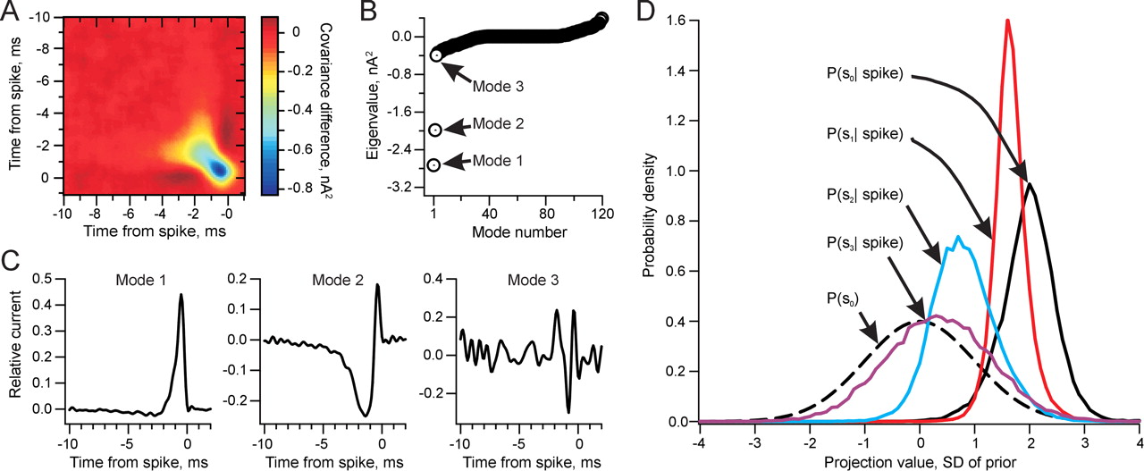
Figure 2B shows the eigenvalues of the covariance matrix (Fig. 2A) measured from the NM responses; there are at least two eigenvalues above the sampling noise. Figure 2C shows the leading three eigenmodes. Mode 1 is similar to the STA but has very little negative fluctuation before the spike time. Considering this feature as a filter of the stimulus, its effect is to locally smooth the input. Thus, one can consider this mode to be a local integrator of current over a short time window. Mode 2 is biphasic, fluctuating from a large, negative component to a small, sharp, positive component. A filter that differentiates the signal is similarly biphasic, but with equal weight in the positive and negative lobes. Although the positive and negative lobes of mode 2 do not precisely sum to zero, it is dominated by a differentiating function. We therefore identify the two eigenvectors as approximately describing an integrating and a differentiating filter on the input. These two modes have a nonzero history of ∼5 ms, consistent with the STA. We note that the width of the positive portion of the STA is less than that of mode 1. The STA is close to a linear combination of the spike-triggering modes and is sharpened with respect to mode 1 by the addition of mode 2 (Agüera y Arcas and Fairhall, 2003). In contrast, mode 3 is noisier, as suggested by its small eigenvalue.
In eight NM neurons analyzed as in Figure 2, the first two modes were highly reproducible, whereas the third mode was variable. Reproducibility among different cells was quantified by projecting the modes from individual neurons onto the average modes of the population. Mode 1 had an average projection (±SEM) of 0.980 ± 0.001 onto the population mean, mode 2 had an average projection of 0.970 ± 0.003, and mode 3 had an average projection of 0.590 ± 0.043 (n = 8).
In two neurons, we added a DC offset (0.25 nA) to the noise stimuli (SD, 1 nA) to produce higher firing rates (98 and 183 Hz). We performed covariance analysis on the data obtained with the DC offset. As in the experiments described above, we found two or three significant spike-triggering modes. The time courses of the modes were not noticeably different from those obtained in other cells at lower rates (range, 20-75 Hz) with no DC offset (data not shown). This suggests that similar features are detected by NM neurons over a wide range of firing rates and mean stimulus levels.

Covariance analysis of spike-triggering currents in an NM neuron. A, Spike-triggered covariance matrix. This matrix represents the average change in covariance of the current stimulus preceding a spike. The covariance difference (color coded) from the prior is plotted versus the times of two stimulus points relative to the spike. B, The eigenvalues of the covariance matrix in A. These values measure the difference in variance along each stimulus dimension between the STE and the entire stimulus ensemble. C, Plots of the first three eigenmodes. Left, Mode 1, the stimulus feature with the largest negative eigenvalue and thus the feature most strongly associated with spiking. Middle and right, Modes 2 and 3, respectively, the second and third most important stimulus features affecting spike probability. D, Probability density of the STE projections onto the STA [P(s0|spike), black] and onto the first three covariance modes [P(s1|spike), red; P(s2|spike), blue; P(s3|spike), purple]. The prior probability density for the STA and all of the modes, P(s0), is plotted with a dashed line. The original stimulus and therefore s0, s1, s2, and s3 are in units of its SD.
The distributions of projections of the STE onto the covariance modes are an indication of their ability to drive spiking. We are looking for differences in the distributions from the Gaussian prior, P(s) = P(s0) = P(s1) = P(s2). The distribution of the STE projections onto modes 1-3, P(s1|spike), P(s2|spike), and P(s3|spike), respectively, as well as that onto the STA, P(s0|spike), are shown along with the prior in Figure 2D. P(s1|spike) has a large, positive mean and reduced SD compared with the prior (mean, 1.92 ± 0.09; SD, 0.27 ± 0.02; n = 8). P(s2|spike) has a smaller mean and larger SD than P(s1|spike), but mode 2 is also clearly significant for spike generation (mean, 0.77 ± 0.08; SD, 0.55 ± 0.02; n = 8). P(s3|spike) has a small mean and slightly reduced SD compared with the prior (mean, 0.30 ± 0.05; SD, 0.92 ± 0.04; n = 8). This shows that mode 3 is only weakly associated with spike generation in NM, so we have limited the covariance-based model to the first two modes.
Construction of one and two feature-based models of NM
We first constructed a model, based on the single STA feature, that takes in an arbitrary stimulus current and outputs instantaneous probability of firing (Fig. 3A) (see Materials and Methods). To implement this model, we first project the stimulus onto the STA. We constructed the threshold function corresponding to this feature by calculating how often a given value of s0 generates a spike (see Materials and Methods). We then took the time-dependent sequence of projection values, s0(t), and at every time t, the instantaneous firing rate was predicted from the corresponding value of the threshold function.
We also constructed a two-dimensional model analogous to the one-dimensional model. In this case, the stimulus is filtered by two features, and so at each time t, the stimulus is described by two projections, s1(t) and s2(t). The nonlinear threshold function is computed from the two-dimensional histograms of the spike-triggered previous and projections, and the firing rate at t is generated by looking up the appropriate value corresponding to [s1(t), s2(t)] (Fig. 3A).
Comparison of the covariance-based, two-dimensional model to the STA-based, one-dimensional model
Figure 3B compares the predicted responses to a Gaussian noise stimulus with the PSTH measured from a neuron by repeated presentation of the stimulus. From a representative 100 ms of experimental data, it is evident that there is very high spike-timing precision. Indeed, the spike-timing jitter was less than could be resolved by the sampling rate of the experiment (10 kHz). Both the one- and two-dimensional models predicted a high firing rate in the vicinity of real spiking in the PSTH, but both models gave broader distributions than the real data (Fig. 3B, right). Neither model totally misses events (“false negatives”), but both models predict some false positives, or firing events not corresponding to the time of real spikes. We quantified the ability of the models to predict spiking by projecting the predicted firing rate onto the true firing rate (PSTH) at different time resolutions. Figure 3C shows these projections versus time resolution. It is evident that both models accurately predict firing, but the two-dimensional model outperformed the one-dimensional model at all time resolutions tested. Neither model was able to predict firing perfectly at very fine time resolution. This limitation may result from the influences of intrinsic noise, nonstationarity, recent spike history, and local adaptation (see Discussion).
Evaluation of the one- and two-dimensional models with information theory
We used information theory to quantify our one- and two-dimensional descriptions of NM neurons. One can use the spikes generated in response to a repeated noise stimulus to compute the mutual information between the stimulus and the occurrence of a single spike. This provides a benchmark with which to compare the performance of the one- and two-dimensional models (Agüera y Arcas et al., 2000). In these experiments, the coefficient of variation of the interspike intervals (0.80 ± 0.02; n = 8) and their approximately exponential distribution (data not shown) are both consistent with nearly independent spiking. Because of the short integration time scales of NM and the relatively moderate firing rates generated under our experimental conditions, we are likely to be very close to the case of truly independent spikes in a real neuron, and the single spike information of Brenner et al. (2000b) is likely to be close to the full information in the spike train computed from finite length “words” (Strong et al., 1998). In this method, we computed the response entropy from the mean rate and the noise entropy from the instantaneous firing rate generated by repeated presentations of the same white noise stimulus (Brenner et al., 2000b). The spike raster plots and the PSTH in Figure 4A indicate that there is very little uncertainty, either in spike-timing jitter or spike number, in NM spike generation at this experimental resolution (0.1 ms). Figure 4B shows an example of the mutual information as a function of time resolution. It indicates that a large percentage of the information is dependent on high time resolution and that the spike train approaches the noiseless limit for information transmission down to 0.1 ms resolution (see Materials and Methods) (Rieke et al., 1997).

Comparison of the one- and two-dimensional model predictions with measured firing rates during Gaussian noise stimulation. A, Top, One-dimensional model of an NM neuron based on the single STA feature. Input current is projected onto the STA. The resulting projection value, s0(t), is mapped into an instantaneous firing rate, r(t), using the measured threshold function. Bottom, Two-dimensional model of an NM neuron based on the first two covariance features. Input current is projected onto modes 1 and 2, and the resulting projection values, s1(t) and s2(t), are mapped into an instantaneous firing rate using the measured 2D threshold function. B, Predictions of the one- and two-dimensional models and the experimentally measured firing rate. The right panels compare these responses on a finer time scale (data from shaded area of the left panels). C, The projection of the one-dimensional model firing rate (gray) and two-dimensional model firing rate (black) onto the measured firing rate from the PSTH versus time resolution. 1D, One-dimensional; 2D, two-dimensional.
We calculated the information captured by the one- and two-dimensional models by comparing the distribution of STE projections onto the features with the prior distribution (i.e., that of the full stimulus played to the neuron) (see Materials and Methods). These information values were nearly constant over a wide range of bin widths used to estimate the distributions (Fig. 4C). We compared the mutual information at the temporal resolution of our experiment, on average 6.7 ± 0.3 bits/spike, with that captured by the one- and two-dimensional models (Fig. 4D) (Agüera y Arcas et al., 2003). The one-dimensional model captured, on average, 62.8 ± 1.2% of the mutual information between the spike train and stimulus, and the two-dimensional model captured 75.4 ± 0.8%, a significant improvement (n = 5; p = 0.0003).
Given the performance of the one- and two-dimensional models in response to Gaussian noise stimuli, stimuli statistically identical to that used to derive the models, we next tested whether the models generalize to stimuli that have been traditionally used to characterize the intrinsic properties of NM neurons: DC steps and sEPSCs. These stimuli are both highly non-Gaussian. We compared these model responses to those obtained in the real neuron from which the models were derived.
DC filtering and temporal precision in NM neurons
NM neurons fire an action potential only to the onset of somatic current steps (Fig. 5A), whereas trains of sEPSCs evoke one-for-one spiking up to 200-300 Hz (Fig. 5B). At 500 Hz, the neuron only fires on 20% of the cycles at steady state (Fig. 5B). Action potentials start to miss cycles in response to higher-frequency sEPSC trains that cause temporal summation of the membrane voltage response (Fig. 5B) (Reyes et al., 1994). This DC or low-frequency filtering is dependent on a large, low-threshold potassium conductance (Reyes et al., 1994; Brew and Forsythe, 1995; Rathouz and Trussell, 1998; Rothman and Manis, 2003). During high-frequency firing, NM neurons show very little spike-timing jitter relative to the onset of each sEPSP (Fig. 5C) (Reyes et al., 1994; Zhang and Trussell, 1994). As the stimulation frequency increases, the average spike latency also increases (Fig. 5C).
Model responses to standard stimuli
We constructed an STA-based, one-dimensional model of the neuron in Figure 5 to predict the instantaneous firing rate of the neuron to the same current stimuli. Figure 6, A and B, display the responses of the model to the same current step and trains of sEPSCs, respectively, used for Figure 5 in the real neuron. The predicted firing rate increases rapidly at the onset of a constant current step but then decreases during the steady-state current. This partly recovers the correct response. However, the model fails to predict the zero firing rate of the real neuron during steady state (DC filtering) (Fig. 6A, right). Furthermore, although the model predicts repetitive firing to phase-locked sEPSC trains, the jitter in spike timing is greater than actually observed (compare Figs. 5C, 6C). For example, when stimulated at 100 Hz, the SD of the experimentally measured response latency curve is <50 μs compared with the one-dimensional model prediction of 190 μs. Unlike in the experiment, the average latency of the model response is relatively constant at all of the frequencies shown (Fig. 6C, dotted lines). The right axis on Figure 6C plots the cumulative probability of spiking for each sEPSP. The model predicts approximately one spike per cycle at 100 Hz but less for higher frequencies. Thus, the first-order description fails to predict some of the correct responses in the real cell.

Evaluation of the one- and two-dimensional models using information. A, Top, Gaussian noise stimulus. Middle, Spike raster from an NM neuron during repeated presentations of the stimulus. Bottom, PSTH formed from the raster. B, The mutual information between the spike train and current stimulus versus time resolution (data points). The solid line represents how the information transmitted varies with resolution for a noiseless neuron (Rieke et al., 1997). C, The mutual information between the spike train and the reduced stimulus, in one dimension (thin) and two dimensions (thick), at the 0.1 ms time resolution. The information is plotted versus the bin width used for the projection values. The dashed lines indicate the stable bin sizes used to calculate the average value. D, The mutual information between the stimulus and the spike train compared with information captured by the one- and two-dimensional descriptions. Error bars show SE. 1D, One-dimensional; 2D, two-dimensional.

Intrinsic firing properties of NM neurons. A, Membrane potential responses (top trace) of an NM neuron to an injected DC step (bottom trace). B, Membrane potential responses (V) to sEPSC trains (I) of increasing frequency (100, 300, and 500 Hz, from top to bottom). The calibration bars in A also apply to B. C, Average response latency to each sEPSC at steady state (50 ms after stimulus onset) for the neuron in B. The firing rate, in 0.1 ms bins, is plotted against the time from sEPSC onset. The dotted lines indicate the mean latencies 0.65, 0.75, and 1.13 ms for the 100, 300, and 500 Hz sEPSC trains, respectively. The SD of the response latencies was <50 μs for the 100 and 300 Hz sEPSC trains and 70 μs for 500 Hz sEPSC train. V, Membrane potential responses; I, sEPSC trains.
We next constructed the two-dimensional, covariance-based model for the same neuron. In Figure 7, A-C, we demonstrate that some of the model predictions are closer to the neural data than those of the one-dimensional description. The two-dimensional model successfully predicts DC filtering, showing a zero firing rate during steady-state current. This phasic response is the outcome of a negative stimulus projection onto mode 2 during steady state, which causes DC filtering even for large current steps (data not shown). Furthermore, the model follows high-frequency sEPSC trains with greater temporal fidelity (Fig. 7B,C). The response of the two-dimensional model to the 100 Hz sEPSC train has a greater maximum firing rate and narrower firing rate distribution relative to the sEPSC onset (SD, 150 μs) (Fig. 7C) compared with the STA model (SD, 190 μs) (Fig. 6C), although not as narrow as the experimental responses (SD, <50 μs) (Fig. 5C). The average response latencies also increase at higher stimulus frequencies (Fig. 5D, dotted lines). However, the firing rates to the 300 and 500 Hz trains are lower than those of the real neuron or the one-dimensional model. This is attributable to the interaction of predictions for closely spaced sEPSCs; the projection values from adjacent sEPSCs overlap and sum linearly. This model treats spikes independently and does not explicitly account for interspike interactions, which are presumably starting to play a role at these stimulus frequencies. We will return to this issue in the Discussion. In addition, the cumulative frequencies in Figure 7C reveal that the two-dimensional model is less responsive than the real neuron, predicting less than one spike per cycle at all frequencies shown.

One-dimensional model responses to DC steps and sEPSCs. A, Model response, r(t), evoked by a DC step, I(t). The right panel shows the response on an expanded time and firing rate axis. The dashed line indicates 0 kHz. B, Model responses, r(t), to sEPSC trains, I(t), of increasing frequency (100, 300, and 500 Hz, from top to bottom). The left scale bars in A also apply to B. C, Average response latency to the sEPSP at steady state (50 ms after stimulus onset) for the model responses in B. The instantaneous firing rate is plotted on the left versus time from the onset of each sEPSC (thick line). The dotted line indicates the mean of the latency distribution (0.81, 0.81, and 0.79 ms for 100, 300, and 500 Hz, respectively). The right axis plots the cumulative frequency (thin line), which measures how many spikes are predicted per stimulus cycle. The sEPSCs have the same amplitude and time course as those in Figure 5. The model was derived from data obtained from the same neuron as that in Figure 5.
The two-dimensional model qualitatively outperformed the one-dimensional model for DC steps, sEPSC trains up to 100 Hz, and Gaussian noise. This two-feature model was more selective for its inputs; it filtered steady-state current and had a narrower temporal distribution of firing rate around sEPSC stimuli.
Pharmacological manipulation of computation in NM
Given the clear qualitative and quantitative picture of the computation of the neuron provided by covariance analysis, we next applied the method to characterize the changes in this computation brought about by pharmacologically induced changes in the intrinsic membrane properties of the neuron. We bath applied DTX, known to block Kv1.1, Kv1.2, and Kv1.6 ion channels (Harvey and Robertson, 2004), to NM neurons. DTX is known to eliminate DC filtering in NM neurons (Brew and Forsythe, 1995; Rathouz and Trussell, 1998). Thus, NM cells treated with DTX have repetitive action potential firing in response to a long constant current stimulus (Fig. 8A, right). The STA in the presence of DTX is decreased in amplitude, slightly longer in duration, and does not have a negative dip preceding the positive going current (Fig. 8B, top and inset). These changes in the STA feature have been interpreted as resulting from an increase in the membrane time constant and a lowering of spike threshold (Svirskis et al., 2004). Furthermore, the nonlinear threshold function obtained during DTX application (Fig. 8C, top) shows a lower threshold than the control. This reflects a decrease in selectivity for the STA feature and an increase in firing rate (9 Hz in control and 75 Hz in DTX).

Two-dimensional model responses to DC steps and sEPSCs. A, Model response, r(t), evoked by a DC step, I(t). The right panel shows the response on an expanded time and firing rate axis. The dashed line indicates 0 kHz. B, Model responses, r(t), to sEPSC trains of increasing frequency (100, 300, and 500 Hz, from top to bottom). The left scale bars in A also apply to B. C, Average response latency to the sEPSC at steady state (50 ms after stimulus onset) for the model responses in B. The instantaneous firing rate is plotted on the left versus time from the onset of each sEPSC (thick line). The dotted line indicates the mean of the latency distribution (0.70, 0.76, and 0.82 ms for the 100, 300, and 500 Hz, respectively). The right axis plots the cumulative frequency (thin line) as in Figure 3. The sEPSCs have the same amplitude and time course as those in Figure 5. The model was derived from data obtained from the neuron in Figure 5.
The two-dimensional description more clearly resolves the change in computation caused by DTX. The first two covariance modes are quite similar before and during DTX application (Fig. 8B, middle and bottom), indicating that the intrinsic temporal filtering properties of the neuron are not significantly altered. What has changed, however, is the threshold function for mode 2 (Fig. 8C, bottom). Recall that because of its monophasic nature, mode 1 operates as a smoothing or integrating filter, whereas mode 2 is biphasic, enacting a differentiating operation. Our results clearly show that the neuron has lost selectivity for the “differentiating” feature that provides the DC filtering property, whereas the selectivity for the integrating feature was only slightly altered (Fig. 8C, middle). This change came about from a shift in the mean of P(s2|spike) in DTX to less than half of that in the control solution (in this cell, 2.03 in control and 0.85 in DTX; 56 ± 5% of control in five cells). The responses of the two-dimensional models (Fig. 8D, top panels) reproduced the change in computation of the real neuron by DC filtering in control (left) and predicting a nonzero firing rate throughout the current step (bottom panels) during DTX application (right). The steady-state response of the two-dimensional, DTX-applied model rose with increasing DC amplitude and began to DC filter at high values of input current (data not shown). This matched qualitatively with the firing responses in the real neuron during DTX application (data not shown). The model responses at onset were also broadened during DTX (Fig. 8, see insets). From covariance analysis, we have resolved the changes in the shape of the STA during DTX application into an unchanged contribution from the integrating mode and a reduced contribution of the differentiating mode.

Pharmacological manipulation of computation in an NM neuron. A, Membrane voltage response of an NM neuron (top traces) before (left) and during (right) bath application of DTX to a DC step (bottom traces). B, The STA (top), mode 1 (middle), and mode 2 (bottom) before (gray) and during (black) DTX application. The inset above the STAs plots them normalized to equal peaks and on a finer time scale to demonstrate the broadening of the STA during DTX application. The dotted line indicates time of spike. C, The nonlinear relationship between the firing rate and the projection of a current stimulus onto the STA (top), mode 1 (middle), and mode 2 (bottom) before (gray) and during (black) DTX application. D, Prediction of the two-dimensional models (top) evoked by a DC step (bottom) from data obtained before (left) and during (right) DTX application. The insets show the model responses on finer time scale and firing rate axes. The dashed line indicates 0 kHz.
Discussion
A goal of single-neuron modeling is to obtain a general quantitative description of the mapping between stimulus and spike output. A complete description should reproduce experimentally measured responses and predict responses to novel stimuli. Even in a single neuron, this is a daunting task; neurons are nonlinear, stochastic, and adapt on many different time scales, making responses both history and context dependent (Shapley and Victor, 1979a; Clague et al., 1997; Sanchez-Vives et al., 2000; Fairhall et al., 2001; Kim and Rieke, 2001; Baccus and Meister, 2002; Truccolo et al., 2005). What makes the problem potentially tractable is that not all possible stimulus fluctuations are relevant for the response of a neuron. Indeed, in the framework we present here, a core component of the computation of a neural system is precisely this reduction of the stimulus to its relevant features. Thus, our task was to find these relevant stimulus features and measure how the neuron computes with them. Ultimately, we aimed to determine how these features and the decision of the neuron to fire depend on the detailed biophysics of the system.
Additional features improve model fidelity
The limitations of a simple single feature (STA) description of spike generation have been demonstrated in the literature in models of single neurons (Agüera y Arcas et al., 2000, 2003; Agüera y Arcas and Fairhall, 2003; Pillow and Simoncelli, 2003) as well as in other systems (Touryan et al., 2002; Fairhall et al., 2003; Petersen and Diamond, 2003; Rust et al., 2005). It has been shown that the assumption of one spike-triggering feature may fail to reproduce measured responses. Covariance analysis was used to systematically determine the significant features of the system, resulting in improved models. For the biophysically realistic Hodgkin-Huxley model, covariance analysis led to a significant improvement over the STA (Agüera y Arcas et al., 2003). In the present study, we have shown this to be the case for a real neuron. NM neurons are selective for at least two features in the input current; a model based on two covariance-derived features captured a significantly higher fraction of the measured mutual information between the noise stimulus and the spike train than the single STA feature. This model more accurately reproduced experimentally measured firing to a noise stimulus. We also tested more traditional stimuli on the model. In contrast to the one-dimensional model, the two-dimensional model correctly DC filtered steps to a steady-state current and responded to a 100 Hz sEPSC train with a higher and more precisely timed firing probability. However, for 300 and 500 Hz sEPSC trains, the STA model predicted the firing rate more accurately than the two-dimensional model. This was a result of a narrower time course of the STA compared with the covariance modes, which reduced interaction between adjacent sEPSCs.
A complete description of the transfer function for a given neuron could be achieved by a quantitative description of the spatial and kinetic properties of the entire membrane. Given such a set of equations, it is possible to determine how the voltage response to a simple input (e.g., a constant current step) depends on the kinetic parameters and the density of ion channels. However, even with such a complete biophysical description, it is very difficult to isolate the role that a given membrane property plays in determining the response of a neuron to a broad set of input statistics. This is a key area in which the covariance method provides not only a simplified description but also insight into neuronal function. Here, we found that pharmacological manipulation of computation in NM had a remarkably simple effect on a two-feature description. Application of DTX decreased the DC filtering property of NM neurons. The two-dimensional model revealed a dramatic change in selectivity for the differentiating feature while the shape of the features stayed similar. The two-dimensional model calculated from data obtained in the presence of DTX reproduced the responses of the manipulated neuron by similarly ceasing to DC filter. More significantly, the two-dimensional description generalizes the DC filtering concept to describe the selectivity of the cell among stimuli other than pure DC steps.
Model limitations
Although covariance analysis provides a significant improvement over the STA-based description, it does not provide a complete solution to input/output properties of neurons. Previous spike history can alter the effect of the stimulus on spike generation (Agüera y Arcas and Fairhall, 2003; Agüera y Arcas et al., 2003; Pillow and Simoncelli, 2003; Paninski et al., 2004; Truccolo et al., 2005). In our example, the NM neuron is unable to fire on every cycle at a 500 Hz stimulation rate (Fig. 5B). Presumably, this is because of refractoriness in spike generation attributable to inactivation of sodium channels. Although the nonmonotonic threshold function enacts some of the effects of refractoriness by enforcing high temporal precision at threshold crossing and suppressing subsequent spikes within a single stimulus fluctuation, we have not dealt explicitly here with spike interactions. In previous work, we have separated stimulus-driven from spike-history-driven effects by analyzing only isolated spikes, those separated by a sufficient interval such that they are statistically independent. Here, our analysis shows that NM neurons compute with current waveforms within a window of ∼5 ms. This limits the effects of spike history in these cells compared with other types of neurons in that most spikes are effectively isolated. However, for high-frequency sEPSC trains, we found that the filter window overlaps with more than one sEPSC, modifying the predicted firing rate without accounting for spike-dependent biophysical changes in membrane potential and conductance. This results in the inability of the two-dimensional model to reproduce the complicated firing pattern of the neuron to a 500 Hz sEPSC train. The present models of neural computation would be improved (but complicated) by explicitly accounting for spike history.
A more subtle issue arises when attempting to predict responses to stimuli that do not occur within the ensemble of stimuli used to derive the model. One would like the model to generate correct responses to arbitrary stimuli, including traditional quasi-static stimuli such as current steps. Although in principle these stimuli are contained within the Gaussian ensemble, in practice they are extreme outliers. In our example, noise with a relatively flat power spectrum out to frequencies of 2 kHz did not efficiently probe the computational changes brought about by DTX. Block of low voltage-activated potassium channels with DTX affects the ability of NM to fire to DC steps, stimuli with relatively high power at low frequencies. Therefore, we used a slower EPSC-filtered noise (see Materials and Methods) to probe the neuron in experiments in which DTX was applied. As a result, the covariance modes were slightly broadened compared with those measured with a faster stimulus. This may have limited our ability to find changes in the time course of the covariance modes brought about by pharmacology. Furthermore, many studies have found that basic neural characterizations in terms of features and static nonlinearity depend on the statistical parameters of the stimulus (Shapley and Victor, 1978, 1979a,b, 1980; Fairhall et al., 2001; Kim and Rieke, 2001; Baccus and Meister, 2002; Serruya et al., 2002; Agüera y Arcas and Fairhall, 2003; Jolivet et al., 2004). Stimuli such as current steps may induce rapid forms of adaptation whereby the filter and threshold function change. Although here we recomputed the model at three other values of mean and SD and found little change, in general such changes can be considered as adaptations and may have information processing benefits for the system. A systematic generalization of covariance methods to arbitrary stimulus ensembles is yet to be determined.
Relevance for auditory processing
Previous work in auditory processing has emphasized the importance of the intrinsic membrane properties of auditory neurons for the preservation and processing of the extremely precise time code present in their input (Reyes et al., 1994; Oertel, 1997; Rathouz and Trussell, 1998; Dodson et al., 2002; Macica et al., 2003; Rothman and Manis, 2003; Svirskis et al., 2004). As noted by several investigators, NM neurons DC filter low-frequency stimuli but have fast channel kinetics to follow high-frequency transient inputs. The combination of these properties allows NM neurons to reliably fire a single action potential to an EPSC, thereby preserving the phase-locked signal in their input while ignoring input patterns that contain little temporal information. Covariance analysis provides quantitative insight into these qualitative aspects of computation. Here, the computation of NM cells is clearly understood as selectivity for an integrating and a differentiating feature in synaptic current. The time course of the features provides a functional measure of the processing time window, whereas the nonlinear threshold function quantifies the selectivity for each feature. The brief duration of these features gives the neuron the ability to compute with high temporal precision. The high selectivity for the differentiating feature gives this cell its DC-filtering property, which only allows firing to transient inputs. This property can be removed by blocking a small subset of ion channels. We expect that future analysis of single neurons using covariance methods will yield fruitful insights about the functional roles of other channel subtypes in neural computation.
Footnotes
This work was supported by a Veterans Affairs Merit Review to W.J.S. and by a Burroughs-Wellcome Careers at the Scientific Interface Award to A.L.F. We thank Fred Rieke and Greg Field for helpful discussions, Ann Simons for help with experimental procedures, and Carol Robbins for technical assistance.
Correspondence should be addressed to Dr. William J. Spain, Department of Neurology (127), 1660 South Columbian Way, Seattle, WA 98108. E-mail: spain{at}u.washington.edu.
Copyright © 2005 Society for Neuroscience 0270-6474/05/259978-11$15.00/0


