

Abstract
The role of irregular cortical firing in neuronal computation is still debated, and it is unclear how signals carried by fluctuating synaptic potentials are decoded by downstream neurons. We examined in vitro frequency versus current (f–I) relationships of layer 5 (L5) pyramidal cells of the rat medial prefrontal cortex (mPFC) using fluctuating stimuli. Studies in the somatosensory cortex show that L5 neurons become insensitive to input fluctuations as input mean increases and that their f–I response becomes linear. In contrast, our results show that mPFC L5 pyramidal neurons retain an increased sensitivity to input fluctuations, whereas their sensitivity to the input mean diminishes to near zero. This implies that the discharge properties of L5 mPFC neurons are well suited to encode input fluctuations rather than input mean in their firing rates, with important consequences for information processing and stability of persistent activity at the network level.
Introduction
Cortical neurons discharge spontaneously in vivo, contributing to irregular background synaptic inputs to other cells (Shadlen and Newsome, 1994). This induces fluctuations in the postsynaptic membrane voltage (Parè et al., 1998) and strongly affects the neuronal frequency versus current (f–I) relationship and input integration (Destexhe et al., 2003). However, it remains unclear whether irregular firing and membrane fluctuations encode relevant information and take active part in signal processing, and whether a neuron can propagate such information to downstream neurons. Associative areas, as the prefrontal cortex (PFC), might be specifically sensitive to input fluctuations to stabilize persistent activity for working memory. In fact, local circuit models of working memory in associative cortices require noisy background environments, weak firing rate accommodation, and saturating synapses [e.g., NMDAR-mediated (Wang, 2001)]. Do prefrontal cortical neurons support specifically the requirements of persistent activity networks, beyond known differences in recurrent connectivity (Elston, 2003)? Is there anything peculiar in the way these neurons respond to input signals?
To address these fundamental issues, we studied in vitro input–output discharge properties of layer 5 (L5) pyramidal cells in the rat medial PFC (mPFC). These cells are the main output stage of the cortical columnar organization. We explicitly recreated an in vivo-like fluctuating current input with independently varying mean and variance. Under similar conditions, it was shown previously that sustained neuronal responses increase monotonically (Ahmed et al., 1998) and become progressively insensitive to the amplitude of input fluctuations in pyramidal cells and fast-spiking interneurons of the somatosensory cortex (SSC) (Rauch et al., 2003; La Camera et al., 2006) as well as in cultured neurons dissociated from the neocortex (Giugliano et al., 2004). This occurs for increasing input offset and results in repetitive and relatively regular firing, mostly independent of the amplitude fluctuations around the offset.
Here, we demonstrate that the predominant discharge response properties of mPFC pyramidal neurons in L5 have an unexpectedly large sensitivity to input fluctuations throughout the range of firing rates sustained by the cell. Moreover, neurons have a sigmoidal f–I response that saturates at relatively low frequencies. To quantify and assess the statistical significance of this single-cell property, we identified the parameters of an extended integrate-and-fire (IF) model, which fit experimental data with high accuracy. In addition, we examined possible candidate subcellular mechanisms underlying this extra sensitivity to input fluctuations by spike-train analysis and additional biophysical modeling. We suggest that a slow component in voltage-dependent inactivation of the Na+ conductance is sufficient to explain the observed sensitivity to fluctuations.
Because persistent firing during delayed-match-to-sample tasks is frequently observed in associative cortical areas rather than in primary sensory areas (Brody et al., 2003), we discuss the impact of the extra sensitivity to the amplitude fluctuations on the stability of persistent activity states in recurrent networks of IF neurons. By using analytical methods, we predict that excitatory networks of mPFC neurons are indeed likely to reproduce more robust persistent states. Finally, we discuss the implication of our results for a novel activity-dependent filtering of information in populations of IF neurons.
Materials and Methods
Slice preparation and electrophysiology.
Tissue preparation was as described by Hempel et al. (2000). Briefly, coronal slices (300 μm) of the prefrontal cortex were prepared from 13- to 50-d-old Wistar rats that were killed by decapitation, following the guidelines of the veterinary office of canton Bern. Whole-cell patch-clamp recordings were made at 32°C from the soma (10–20 MΩ access resistance) using a BVC-700A bridge amplifier (Dagan, Minneapolis, MN). Bridge balance and capacitance neutralization were applied. Hyperpolarizing and depolarizing current steps were also used to obtain estimates of the passive properties of patched neurons (Iansek and Redman, 1973), such as the total membrane capacitance Cm and apparent input resistance R in.
Chemicals and solutions.
Slices were continuously perfused with artificial CSF (ACSF) containing the following (in mm): 125 NaCl, 25 NaHCO3, 2.5 KCl, 1.25 NaH2PO4, 2 CaCl2, 1 MgCl2, and 25 glucose; solutions were balanced with 95% O2 and 5% CO2. The pipette solution contained the following (in mm): 115 K-gluconate, 20 KCl, 10 HEPES, 4 ATP-Mg, 0.3 Na2-GTP, and 10 Na2-Phosphocreatine with pH adjusted to 7.3 via KOH. Other pipette solutions were reported not to significantly alter the response properties of the cells under similar experimental conditions and for the same current-clamp protocol (Rauch et al., 2003). In some experiments, synaptic inputs were blocked by adding selective antagonists of ligand-gated channels to the bath (i.e., APV, 50 μm; CNQX, 10 μm; GABAzine, 3 μm). This did not affect the input–output response properties of the cells investigated in this work. All of the chemicals were obtained from Sigma (St. Louis, MO) or Merck (Geneva, Switzerland).
Noisy stimulation protocol.
In all of our experiments, we used a current-clamp stimulation protocol. It consisted of a repeated injection into the soma of pyramidal neurons of independent fluctuating current waveforms I(t), each lasting 10 s and interleaved by 30–60 s of recovery time (Mainen and Sejnowski, 1995; Poliakov et al., 1997; Destexhe et al., 2001; Protopapas and Bower, 2001; Fuhrmann et al., 2002; Chance et al., 2002; Shu et al., 2003; Silberberg et al., 2004). When a neuron embedded in large neocortical networks receives a barrage of synaptic inputs through synapses with small efficacies compared with the firing threshold, the resulting currents can be well approximated by an input current with random Gaussian fluctuations of variance, s
2, around the mean, m (Tuckwell, 1988; Renart et al., 2003). Therefore, I(t) was synthesized as Gaussian noise. If postsynaptic currents are instantaneous, I(t) is white noise, whereas for exponentially decaying synaptic currents, I(t) is colored noise with a correlation time length equal to the synaptic decay time constant. The following iterative expression was used to synthesize I(t), a realization of an Ornstein–Uhlenbeck process (Cox and Miller, 1965), as follows:
 which represents the exponential filtering of a Gaussian white noise.
In Equation 1, ζt represents a random variable from a normal distribution (Press et al., 1992), and it was updated at a rate of 5–10 kHz (i.e., dt = 0.1–0.2 ms). τ1 represents the correlation time length of the noise, and it accounts for the effective decay time constant of individual EPSCs/IPSCs. Restricting our interests to the contribution of AMPA- and GABAA-mediated fast synaptic currents, τ1 was fixed to 3–5 ms (Destexhe et al., 1994). The exploration of the stimulus space (m, s) was performed interactively in a shuffled order, randomly repeating some of the pairs (m, s), and independently varying m and s across subsequent stimulation trials (see Fig. 1). The entire procedure typically required 30–60 min of recording time to be completed. The reproducibility of the neuronal discharge rate to the same input statistics (m, s) was regularly tested. In addition, the stability of the resting membrane potential Em and of the cell input resistance R in were continuously monitored. The protocol was stopped in the case of drifts in any of these observables.
Analysis of the evoked discharge response.
Intracellular voltage responses to each current stimulus, characterized by the pair (m, s), were collected. Individual spike times and shapes were extracted from raw traces and processed by custom software in MatLab (MathWorks, Natick, MA).
The discharge frequency of the neuron (f) was calculated by counting spikes in two consecutive and nonoverlapping time windows, thereby characterizing transient and steady state responses. The transient response was evaluated by measuring the mean firing rate during the first 2–2.5 s of stimulation, whereas the steady state response refers to the last 5–8 s of stimulation; corresponding temporal windows were averaged across the available repetitions. Experimental curves [fh = fh (mh , sh ), h = 1, 2, …, M] were obtained for two to four distinct values of s and M ∼ 20. These curves were plotted and compared with the theoretical responses of IF model neurons (Tuckwell, 1988) driven by the same fluctuating currents. Recordings were further compared with available data for pyramidal L5 neurons in the somatosensory cortex (Rauch et al., 2003) and for dissociated cortical neurons in culture (Giugliano et al., 2004).
When approximating the membrane voltage distributions that result from incoming synaptic noise, a current-based model that neglects conductance fluctuations gives similar results to conductance-based models, under the effective membrane time constant approximation (Richardson, 2004; Richardson and Gerstner, 2005). However, significant differences between the irregularity of the spike trains evoked under the two conditions were reported (Rudolph and Destexhe, 2003a), together with distinct capabilities of resolving temporal inputs (Hô and Destexhe, 2000; Rudolph and Destexhe, 2003b). Nevertheless, the parameters of current-driven and conductance-driven stimulations can be selected to result in overlapping f–I transfer functions as long as the mean firing rate is the relevant observable (Rauch et al., 2003; La Camera et al., 2004b), as in our study.
Models response function.
Analytical expressions of the current-to-rate response function f = ΦIF(m, s) for the leaky IF (LIF) neuron (Tuckwell, 1988), as well as for our extension of it (sLIF), were used to optimally fit these models to the experimental data of each cell. The analytical expression for the models f–I stationary response is given by the following (Ricciardi, 1977):
 where C indicates the membrane capacitance, μ = m/C, and τ is the membrane time constant. τω represents the absolute refractory period and, for conventional IF models, it is usually assumed to be constant. For our extended model (sLIF), an additional dependence of f on the amplitude of the noise s was considered, making the absolute refractory period inversely depend on s:

In Equation 3, both τarp and ω are positive constants, with ω quantifying the degree of divergence between f–I relationships, whereas τarp −1 acts as an upper bound for the firing rate (see Figs. 3, 5). Because LIF and sLIF differ exclusively in the convergence or divergence of the f–I curves for distinct values of s, for ω = 0 ms pA, the models are equivalent. Therefore, the high statistical significance of model fits by one model but not by the other allowed us to test the significance of the divergence of the f–I curves found in the experiments, as well as to quantify it by the best-fit values of ω.
Finally, a minimal model of spike-frequency adaptation (La Camera et al., 2004) was included at the steady state to capture the effect of sodium- or calcium-activated potassium currents. Analytically, it results in an implicit dependence of μ on the firing rate f = ΦIF, weighted by a positive constant α that quantifies the amount of spike-frequency adaptation:

In the model, the resting membrane potential was 0 mV, and the constant threshold θ was fixed 20 mV above rest (i.e., E = 0 mV and θ = E + 20 mV). The reset voltage H after each spike was a free parameter. Thus, the model was characterized by five independent parameters (or six when adaptation was included and thus α ≠ 0).
An alternative IF model with constant leak and spike refractory period similar to the LIF model [i.e., CLIFF (Fusi and Mattia, 1999)] was also considered and performed similarly to the LIF model (data not shown).
Statistics.
For each cell, the χ2 test was applied as a quantitative indication of the goodness-of-fit of the IF models (i.e., LIF and sLIF) (Press et al., 1992). χ2 and its minimum χmin2 are random variables approximately distributed according to a χ2 distribution. This makes p χ = Prob(χ2 > χmin2) a standard indicator of the significance and quality of the fit. In addition, a measure of the narrowest confidence interval for each data point corresponding to a successful χ2 test with p χ > 0.1, was chosen as a quantitative analog of the quality of the fit [i.e., K (see Eq. S2, available at www.jneurosci.org as supplemental material)] and was used to compare the performance of distinct IF models (i.e., LIF and sLIF) in describing the entire data set (see Fig. 4).
For the evaluation of p χ, the degrees of freedom (DoF) of the χ2 distribution were selected according to the model in use. In each experiment, the DoF corresponded to the difference between the number of free parameters of the model to be identified and the number M of available experimental observations for a given cell. A model incorporating more parameters will pass the statistical test with increased difficulty compared with a model with fewer parameters, for a given data set (Press et al., 1992). With the aim of directly comparing our findings to previous work and explicitly challenging our new sLIF model, we chose the strictest criteria discussed by Rauch et al. (2003). Therefore, the fits were accepted only when p χ > 0.1. When p χ was smaller, the discrepancies between the data and the model predictions were assumed unlikely to be chance fluctuations (within the confidence intervals), and the fit was rejected.
Finally, the Pearson correlation coefficient and the Kendallapos;s Tau nonparametric (rank-order) test were used to assess statistical correlations (Press et al., 1992). The latter provides a correlation measure rK together with an estimated significance level pK , which represents the false positive probability (i.e., the probability of obtaining the same value for rK from statistically independent samples).
Biophysical modeling.
Experimental results were compared with qualitative predictions of two single-compartmental conductance-based model neurons: a Hodgkin–Huxley (HH) and a neocortical model neuron. The HH model neuron (Hodgkin and Huxley, 1952) included a slow sodium inactivation gate i with rate functions described by Miles et al. (2005): α i (V) = 0.0077/[1 + exp(−2 + V/9)] and β i (V) = 0.0077 [1 + exp(2 − V/9)]. Similar results were also obtained with rate functions for the slow sodium inactivation gate i as described by Fleidervish et al. (1996). Other equations and parameters were as typically defined for the HH neuron (Hodgkin and Huxley, 1952; Koch, 1999; Dayan and Abbott, 2001; Gerstner and Kistler, 2002): the capacity of the membrane was 1 μF/cm2; leak, sodium, and potassium currents had maximal conductances of 0.3, 120, and 36 mS/cm2, respectively, whereas their reversal potentials were −54, 50, and −77 mV, respectively. Neuronal surface area was assumed to be 0.004 mm2. The neocortical model neuron was based on one described by Gerstner and Kistler (2002), which is a slightly modified version of the model presented by Erisir et al. (1999); this model includes fast and slow potassium currents, a fast sodium current, and a leak current. For this model, leak, sodium, fast potassium, and slow potassium currents had maximal conductances of 0.25, 50–60, 225, and 0.225 mS/cm2, respectively, whereas their reversal potentials were −70, 74, −90, and −90 mV, respectively. The capacity of the membrane and the neuronal surface area were chosen as for the HH model.
To this model, as with the HH model, we added a slow sodium inactivation gate i with rate functions based on neocortical neurons as described by Fleidervish et al. (1996), α i (V) = 0.001 exp[(−85 − V)/30] and β i (V) = 0.0034/(1 + exp[(−17 − V)/10]).
Equations were solved numerically by MatLab and compiled C code using fourth-order Runge–Kutta integration with a fixed time step of 0.05 and 0.005 ms for the HH and neocortical models, respectively. Injected current stimuli were computed by Equation 2 with τ I = 1 ms.
Spike times were identified as the upward crossing of the voltage trace at −20 mV with resting potentials of −65 and −70 mV for the HH and neocortical models, respectively. Firing rates for a given input current were measured at steady state.
Simulation code is available for the NEURON simulation environment (Carnevale and Hines, 2006) on the SenseLab ModelDB database (http://senselab.med.yale.edu/senselab/modeldb, n. 83590).
Analysis of recurrent networks of IF neurons.
By the extended mean-field theory (Amit and Brunel, 1997a; Brunel, 2000; Mattia and Del Giudice, 2002), which allows one to investigate the collective activity of randomly interconnected population of neurons from the knowledge of their f–I curves, we analytically studied and compared populations of IF neurons characterized by the divergent f–I curves (sLIF) to populations of conventional leaky IF neurons (LIF). We considered homogeneous networks of N
e excitatory neurons, using Equations 2 and 3 as the single-neuron f–I curve with the effective parameters identified in our experiments (Table 1) or in a previous report (Rauch et al., 2003). We neglected network heterogeneities to keep the interpretation of the results as simple as possible (but see Amit and Brunel, 1997b). We chose an unstructured connection topology with random probability of synaptic connection between any two neurons C
ee = 0.1. The total synaptic current (i.e., the mean field) experienced by a generic neuron results from recurrent and background contributions, and its statistics is assumed to be Gaussian distributed, described by mean m(f) and variance s
2(f) (Amit and Brunel, 1997a; Rauch et al., 2003):
 where f indicates the network mean firing rate. J is the effective peak amplitude for the individual EPSCs, which decay with time constant τ
e
. Both J and τ
e
were assumed to be uniform across all of the synapses of the network, and τ
e
was set to the same values of τ
I
(Eq. 1). m
0 and s
0
2 are two fixed parameters, corresponding to the effect of background synaptic activity and feedforward inputs, independent of f.
where f indicates the network mean firing rate. J is the effective peak amplitude for the individual EPSCs, which decay with time constant τ
e
. Both J and τ
e
were assumed to be uniform across all of the synapses of the network, and τ
e
was set to the same values of τ
I
(Eq. 1). m
0 and s
0
2 are two fixed parameters, corresponding to the effect of background synaptic activity and feedforward inputs, independent of f.
Numerical values of the best-fit parameters for the sLIF model
In Figure 8, persistent activity states were investigated by studying the solutions f* of the implicit equation
 that satisfy the stability condition dΦIF/df < 1.
In Figure 9, input–output network transformations were approximated by examining slow modulations Δf(t) around two working points f* [i.e., f = f* + Δf(t)], f* = f up and f* = f down, assumed to be persistent states of an appropriate (unmodeled) larger network. Output modulations were assumed to result from a slow and weak modulation in the feedforward input component around fixed values [i.e., m 0(t) = m up/down + Δm(t) and s 0 2(t) = s up/down 2 + Δs 2(t)] and computed by f = ΦIF[m(f*), s(f*)] without solving the self-consistency. Therefore, we assumed that Δm(t) and Δs 2(t) were weak enough to allow the network to persist in its equilibria states.
Results
To explore the impact of irregular cortical synaptic inputs on the single-neuron response properties in the rat mPFC, we introduced current-clamp fluctuating stimuli in single neurons in vitro, and we observed the evoked firing response. Such a stimulation protocol approximates the barrage from in vivo firing populations of excitatory and inhibitory presynaptic neurons (Destexhe et al., 2001; Rauch et al., 2003; La Camera et al., 2006). In brief, the firing of excitatory and inhibitory afferent populations is replicated by a filtered Gaussian current (Tuckwell, 1988) that was injected somatically. Both mean m and variance s 2 of such current stimuli relate to each other, both depending on the number, activation rate, and synaptic current amplitudes at the soma of many simulated afferents, which fire as independent random Poisson processes (Renart et al., 2003). Because we aimed to study how varying the level of input fluctuations affects neuronal responses at low and high mean currents, stimulus mean m and variance s 2 were varied independently while measuring the mean firing rate (Figs. 1, 2).

The neuronal discharge response retains sensitivity to input fluctuations as demonstrated by diverging f–I curves for distinct levels. A , B , The discharge response of a typical layer 5 pyramidal neuron of rat medial prefrontal cortex was quantified in terms of the mean firing rate f ( A ) and the coefficient of variation (CV) of the interspike intervals ( B ) as a function of the input current mean m. Different colors and marker shapes represent different values of the amplitude fluctuations in the input current, where SD s is 50, 150, and 300 pA (see inset in top left panel). Curves remain well separated from each other (i.e., divergent) throughout the range of m. C , For each combination (m, s), the evoked spike trains were studied at the steady state while carefully monitoring the stationarity of the spike shape at the beginning and at the end of the trace (boxes).

f–I curves, averaged across 80 individual cells, display divergence. Transient individual mean rate responses, obtained for a set of 80 L5 pyramidal cells (as in Fig. 6), were averaged by first shifting to the left each data point proportionally to the cell input resistance, R in. Such normalization acts as an indirect estimate of the rheobase current, m rhe. The stimulus parameters m were associated together in bins of 100 pA, whereas error bars represent the SE across the data points available in each bin (marker shapes and colors are as in Fig. 1, with s binned as 50, 100, and 300 pA). Very similar average curves were obtained analyzing steady-state responses.
The results described below are based on whole-cell somatic recordings obtained from 113 pyramidal cells in mPFC slices. Large L5 regular spiking pyramidal neurons with a thick apical dendrite were identified by their morphology and electrophysiological response properties (Zhang, 2004) and selected for recording. In some experiments, biocytin histochemistry was used to confirm the cortical layer and cell type as well as to check whether the entire neuronal apical dendrite was in the plane of the slice and whether this had any impact on our results (see supplemental material, available at www.jneurosci.org).
Our observations are based on the analysis of both steady-state and transient neuronal response properties, which showed very similar trends.
The resting membrane potential, total membrane capacitance, and apparent input resistance were estimated as (mean ± SD) Em = −69.87 ± 5.46 mV, Cm = 222.84 ± 95.66 pF, and R in = 107.36 ± 60.77 MΩ (i.e., R in Cm = 23.33 ± 7.67 ms), respectively. All cells had action potentials characterized by overshoot and maximal upstroke and downstroke velocities of 26.1 ± 10.6 mV, 127.5 ± 53.1 mV/ms, and −43.3 ± 22.5 mV/ms, respectively, averaged across all stimulation trials from all experiments.
mPFC pyramidal cells display increased sensitivity to noise
Transient and steady-state firing f–I relationships were evaluated using noisy current steps of 10 s duration while sweeping the input current mean m and variance s 2 independently (Figs. 1, 2). Figure 1 reports the results of a typical experiment where raw voltage traces and steady-state analyzed f–I curves are shown. When the input current mean m was larger than the minimal DC step amplitude needed to evoke a spike (i.e., the rheobase current; m = m rhe; s = 0), cells fired more regularly than for lower means m (Fig. 1 B,C). Firing rate was also increasing with m. Under the same experimental conditions, previous studies reported that the mean firing rate of SSC pyramidal cells and fast-spiking interneurons become generally insensitive to input fluctuations s while linearly increasing for increasing current mean m (Rauch et al., 2003; La Camera et al., 2006) (Fig. 3).

Summary of the observed f–I curve divergence and comparison with previous results from L5 somatosensory cortex. Firing f–I curves from pyramidal neurons have been summarized by a parameter that quantifies their shape: the divergence parameter ω (see Materials and Methods). L5 cells of the somatosensory cortex generally showed no divergence (ω = 0) and were previously reported to become insensitive to s for increasing input current means m (Rauch et al., 2003; La Camera et al., 2006). Conversely, mPFC L5 pyramidal cells display a heterogeneous degree of divergence, as shown in the distribution histogram. Sketches for the cases ω = 8 and ω = 50 were reported for the sake of comparison.
L5 mPFC pyramidal neurons instead showed a prominent sigmoidal saturation of the mean firing rate with maximal firing frequency ∼40–60 Hz, for increasing values of m. In addition, individual f–I curves obtained in the same neuron for distinct values of s showed an unexpected divergence. mPFC neurons thus retain a high sensitivity to fluctuations of the input current (Figs. 2, 3) throughout the range of input mean for which a firing response can be sustained (i.e., −200 pA to 1200 pA). This has been summarized in Figure 2 for a population of 80 different cells where the transient f–I responses have been studied. In contrast, neuronal sensitivity to the input mean is reduced for values of m above saturation (i.e., > 0.2–0.5 nA) as curves plateau.
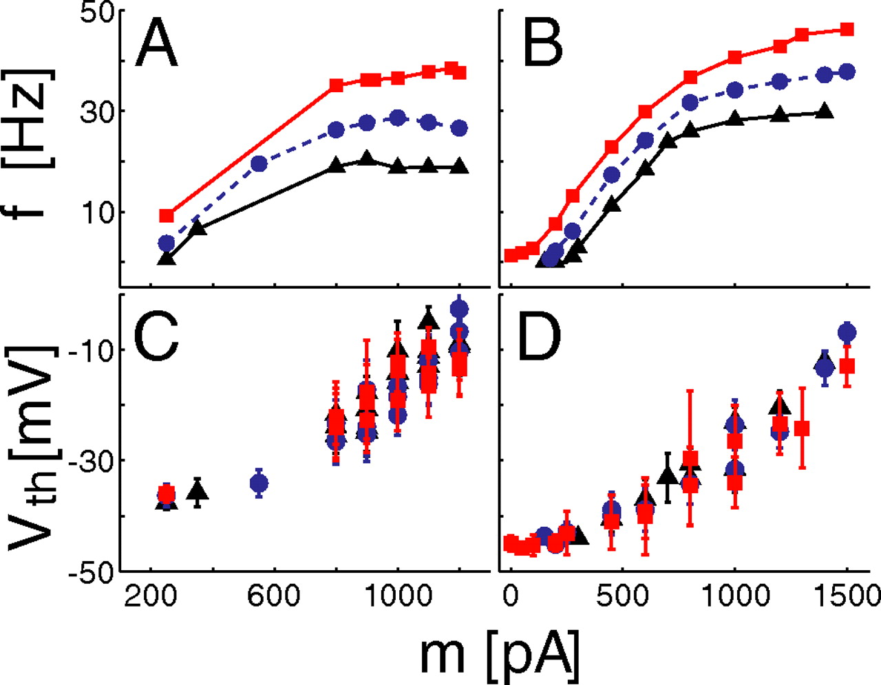
Firing rate saturation and increased sensitivity to input fluctuations were accompanied to a positive shift of the apparent voltage spike-threshold V th. This was defined as the average of the values of the membrane potential V, corresponding to a rate of change dV/dt of 10 mV/ms during each action potential. Figure 4 reports and compares the f–I curves and the dependence on m and s of the spike threshold V th in two typical examples. The spike threshold increases with m regardless of s as the f–I curves saturate. This suggests that the cellular mechanisms underlying spike generation might be responsible for the divergence of these f–I curves (see Materials and Methods, Biophysical modeling).

Sensitivity to input fluctuations correlates with a modulation of the spike threshold. A–D , Panels report and compare the f–I relationships of two cells ( A , B ) with the steady-state spike threshold V th as a function of the input current mean m ( C , D ) (marker shapes and colors are as in Fig. 1). This was defined as the value of the membrane voltage V that corresponds to a rate of change dV/dt of 10 mV/ms. The steepest increase of V th on m occurs in the range of saturation for the f–I curves, allowing the firing of the neuron to become sensitive to s rather than to m.
mPFC pyramidal cells respond as integrate-and-fire neurons
To assess the statistical significance of the f–I curve divergence observed in mPFC pyramidal neurons, we considered IF neurons. These models have been found to approximate very well the response properties of cortical neurons (Rauch et al., 2003; Giugliano et al., 2004; Jolivet et al., 2006; La Camera et al., 2006) and more biophysically detailed model neurons (Fourcaud-Trocmé et al., 2003; Jolivet and Gerstner, 2004; Brette and Gerstner, 2005). IF models generally include a fixed absolute refractory period T arp after spike emission. This results in a maximal firing frequency of 1/T arp, irrespectively of s and thus leading to converging f–I curves. Here, we considered two IF models with different forms of refractoriness and fit these two models to data from each cell (see Eqs. 2, 3). We found that only the IF model incorporating a fluctuation-dependent refractory period fit the data well (Figs. 5, 6).

Divergent f–I curves are captured by a novel integrate-and-fire model used to quantify the statistical significance of the discharge sensitivity to input fluctuations. Panels report results from four different cells as in Figure 1, two under control ACSF and two under pharmacological blockade of synaptic receptors, from top to bottom, respectively. Discharge responses were evaluated over the first 2 s of stimulation as a function of the input current mean m and variance s 2; marker shapes and colors are as in Figure 1 (50, 150, and 300 pA). Transient and steady-state f–I revealed the same degree of divergence. The f–I curves corresponding to distinct levels of input fluctuations s are well approximated by the extended (sLIF) integrate-and-fire dynamics but not by the conventional LIF model. Responses were compared with the best-fit predictions (lines) provided by the novel (left) and the conventional IF (right) model. Whereas the χ2 test was always well above significance for the sLIF (i.e., p χ > 0.1), the LIF model gave f–I curves that differed from experimental data, as apparent from the increased mean absolute error e and by inspection.

The significance of f–I curve divergence was quantified by the superior fit performance of the model incorporating the extrasensitivity to input fluctuations. This plot displays the goodness of model fits between the extended (sLIF) and conventional (LIF) leaky integrate-and-fire models and data from 80 cells recorded over the first 2 s of stimulation without pharmacological blockers. For each cell, the performance was related to the narrowest confidence interval, corresponding to a successful χ2 test with p χ > 0.1 (see Results and Eq. S2). K is the number of SDs used to compute statistical confidence for each data point. K ≤ 1 was chosen as the condition for significance (dashed line) to facilitate comparison with previous reports in the literature.
For most of the cells, the performance for f = ΦIF(m, s) of an IF model (Eq. 2) fitting the experimental data were high and statistically significant only if the model was extended to include an extra sensitivity to s (Eq. 3).
Across all of the experiments, no cell was better fit by the conventional LIF. Of 80 cells recorded without synaptic blockers in the ACSF, the transient discharge response in 73 (91%) could be fit (i.e., p χ > 0.1, by the χ2 test with K ≤ 1) (see supplemental material, available at www.jneurosci.org) when the extended model (sLIF) was used; spike-frequency adaptation (Eq. 4) was unnecessary for successful fits during the transient period (i.e., α = 0). Twenty-seven of 80 cells (33%) could be fit by both the new model (sLIF) and the conventional leaky IF (LIF). Similarly, considering the steady-state response, 51 of 80 (64%) cells could be fit only by the extended model, whereas 13 of 80 (16%) were fit equally well by both models. A comparably strong difference between the performance of the two models holds for cells recorded under pharmacological blockade of synaptic receptors (n = 9) [for transient, 9 of 9 (100%) fit by extended model, 1 of 9 (11%) fit by both models; for steady state, 4 of 9 (44%) fit by extended model, 1 of 9 (11%) fit by both models].
In Figure 5, the fit performance of the two models to the f–I curves of four typical cells was compared. It is apparent that only the response functions of the sLIF model (Fig. 5, left column) show divergence and thus capture the extra sensitivity to input current fluctuations that are evident in the data, whereas for the conventional LIF model, the response functions converge to a common trajectory (Fig. 5, right column) regardless of s.
In addition, Figure 6 summarizes the overall fit performance by an analog indicator of goodness-of-fit, related to the narrowest confidence interval for each data point corresponding to a successful χ2 test (p χ > 0.1) (see Materials and Methods). The value K = 1 (K = 2) gives a confidence level of ∼68% (95%), which describes the variance allowed for the data as calculated via δh± (Eq. S2) (Rauch et al., 2003; La Camera et al., 2006). Therefore, a fit passing the test with K = 0.5 captures the data with better accuracy, because the data variance is smaller than one with K = 0.9.
Quantification of the sensitivity to fluctuations
We could quantify the sensitivity of the cells to input fluctuations by examining the best-fit model parameter ω from the sLIF model and assess the heterogeneity of cells with regard to the degree of this sensitivity (Fig. 3). Table 1 summarizes the best-fit sLIF model parameters across all of the cells, reporting the ensemble mean and SD of each parameter. From Equation 3, it is apparent that two parameters, τarp and ω, primarily determine the shape of the f–I curve and its sensitivity to the input fluctuations; τarp sets the maximal firing rate, and ω is related to the divergence of the f–I curves in response to different levels of input fluctuations s. Interestingly, the coefficient of variation of τarp was quite low (i.e., ∼30% for both transient and steady state), whereas the coefficient of variability of ω was almost five times higher (i.e., ∼140% for both transient and steady state). Because τarp and ω were only weakly correlated to each other [Kendallapos;s tau rank order test, rK = 0.14, pK = 0.03 (transient); rK = 0.1, pK = 0.15 (steady state)] (see supplemental material, available at www.jneurosci.org), the large variability of ω suggests that L5 pyramidal cells show differing degrees of sensitivity to noise, and this explains why a fraction of the cells could be fit equally well by both LIF and sLIF models. The best-fit parameter ω was weakly correlated with respect to the direct estimates of the input resistances of the cells (Kendallapos;s tau test, rK = 0.25, pK < 0.001) and to their membrane time constants τ m (Kendallapos;s tau test, rK = 0.19, pK < 0.1); it was not significantly correlated to membrane capacitances Cm .
As expected, the correlation between the model parameters identified in the transient and those identified in steady state was very strong. In addition, the linear correlation coefficient between the membrane time constant τ m , which was directly estimated in each experiment, and the corresponding sLIF effective parameter τ was 0.33 (Kendallapos;s tau test, rK = 0.31 with pK = 0.003). The correlation coefficient between the membrane capacitance and the corresponding sLIF effective parameter C was 0.55 (Kendallapos;s tau test, rK = 0.43 with pK < 0.0001).
Slow sodium inactivation and sensitivity to fluctuations
Divergent f–I relationships demonstrate the increased sensitivity to input fluctuations of these cells. Whereas the underlying mechanism is unknown, this sensitivity implies that these neurons adapt to the offset of the input (i.e., the mean), without adapting to rapid changes in the input (i.e., the variance).
Biophysically, we expect that this adaptation depends on multiple channels, and there is some evidence, for example, that slow afterhyperpolarizations are indirectly involved (Higgs et al., 2006). However, using simple biophysical models such as the Connor–Stevens, Traub–Miles, and Hodgkin–Huxley model neurons, we find that steady-state divergent f–I curves, in general, do not result directly from additional slow voltage- or calcium-dependent potassium channels (data not shown). These currents can indeed encourage a neuron to respond to high-frequency fluctuations while preventing a response to DC offsets, but their effect is only transient. These currents linearize the stationary f–I curves (Ermentrout, 1998) and decrease their slopes regardless of the input fluctuations (La Camera et al., 2004a). Some authors suggest that spike-frequency adaptation resulting from these currents is weaker in the presence of noise and irregular neuronal discharge (Tang et al., 1997; Destexhe and Paré, 1999). Stronger noise might therefore evoke weaker adaptation currents, producing divergent f–I curves. However, this occurs in the noise-dominated regime (m < m rhe). We studied models similar to those by Tang et al. (1997) but failed to observe divergence of f–I curves in the drift-dominated regimes (i.e., m > m rhe). Furthermore, introducing in a LIF model several adaptation currents acting on multiple time scales (Descalzo et al., 2005; Drew and Abbott, 2006; La Camera et al., 2006) could not replicate the f–I divergence observed in the experiments (data not shown).
Divergence occurs when the neuron adapts preferentially to slow rather than fast components of the input. We demonstrate this point by incorporating slow voltage-dependent sodium inactivation into the Hodgkin–Huxley model as well as into a “nonadapting” neocortical point neuron model (see Materials and Methods) and showing that this addition changes the f–I curves from convergent to divergent (Fig. 7).

Slow sodium inactivation is sufficient to account for f–I curve divergence in biophysical models of action potential generation. A , B , Introducing slow sodium inactivation and its recovery process (Fleidervish et al., 1996; Miles et al., 2005) in the standard Hodking–Huxley model ( A ) and in a neocortical point neuron (see Materials and Methods) ( B ) causes the neuron to effectively modulate its firing threshold in response to slow components of the input current. The plots replicate the experimental protocol of Figure 1 A for the Hodgkin–Huxley and neocortical models with (solid lines) and without (dotted lines) the slow sodium inactivation. s was set to [64 96 128] pA in A and [80 120 160] pA in B . Colors are as in Figures 1, 2, S1, and S2.
By including a description of slow sodium inactivation and its recovery process, the model neuron effectively modulates its firing threshold in response to slow components of the input current (i.e., the DC component), because sodium inactivation is voltage dependent with a time constant slower than sodium activation. Thus, in its adapted state, the initiation of an action potential becomes relatively more sensitive to input fluctuations and the statistical distribution of the fluctuations and less sensitive to slow components of the input current. The critical factor underlying divergent f–I curves evidently relates to the spike-generating mechanism, where low sodium conductance is a mechanism of spike frequency adaptation (Melnick et al., 2004) and slow sodium inactivation is one way of modulating the sodium conductance (Fleidervish et al., 1996).
Indeed, by arbitrarily defining the spike threshold as the voltage V th corresponding to a rate of change dV/dt exceeding 10 mV/ms, our experimental recordings revealed a monotonic increase of V th as a function of m (Fig. 4 C,D). As expected, the steepest increase of V th on m occurs in the range of divergence for the f–I curves (Fig. 4 A,B). Together with a very slow component of spike frequency adaptation and with the progressive decrease of the maximal upstroke velocity of each action potential as a function of time (data not shown), this suggests the presence of a slow inactivation of sodium currents. That slow inactivation of sodium currents might prevent high-frequency responses to slow depolarizations has been suggested previously (Fleidervish et al., 1996), and here we indicate this as a putative mechanism for divergent f–I curves with high values of mean current m. To a first approximation, this slow inactivation mechanism allows the firing threshold to adapt to m and thus extends the dynamical range of the sodium fast inactivation component and its fast voltage-dependent recovery, which is by definition sensitive to fast input fluctuations (i.e., s). Under these conditions, the resulting firing refractoriness is mostly dependent on s, rather than m, even in the drift-dominated regime (i.e., m > m rhe). We thus speculate that slow sodium inactivation is functionally similar to the fluctuation-dependent refractory period that was explicitly included in the sLIF model as a phenomenological parameter.
Finally, dendritic calcium electrogenesis was deemed unlikely to contribute to the increased sensitivity to fluctuations (see supplemental material, available at www.jneurosci.org), suggesting that somatic mechanisms alone suffice. In fact, we examined a posteriori those experiments where the apical dendrite was cut during the slicing procedure and systematically analyzed spike trains, where we looked for, but failed to find, conditions necessary for supralinear dendritic calcium spikes (Larkum et al., 1999, 2004).
Implications for persistent activity in recurrent mPFC networks
We studied the stability of dynamical states in homogeneous recurrent networks of IF model neurons with divergent and convergent f–I curves using the best-fit parameters identified in the experiments and mean-field analysis (Renart et al., 2003). Random networks of recurrently connected excitatory model neurons are known to show a bistable regime for a limited range of the effective synaptic coupling J (Fusi and Mattia, 1999). This kind of persistent activity emerges as a population effect, and it can coexist with a global spontaneous activity state (Amit and Brunel, 1997a). This appears as a consequence of the appropriate balance between the strength of background and recurrent inputs. In fact, recurrent inputs can consistently maintain the overall input to a neuron (Amit and Brunel, 1997a), thereby resulting in a self-sustained network state. Similar synaptic reverberations are considered as a candidate underlying mechanism for mnemonic persistent neuronal firing observed in associative cortical areas during delayed-match-to-sample tasks (Wang, 2001; Renart et al., 2007).
By mean-field analysis, persistent activity states can be searched as stable solutions f* of a self-consistent equation (Eqs. 2 –6). Parameters such as the strength of synaptic coupling J and of the background (i.e., feedforward) inputs m 0 and s 0 (Eq. 5) can be varied while computing existence and location of f*. Persistent activity states were represented in Figure 8 A as a bifurcation diagram, where the values f corresponding to stable mean firing states were plotted as a function of J and denoted by a solid line. Unstable solutions were instead denoted by a dashed gray line.
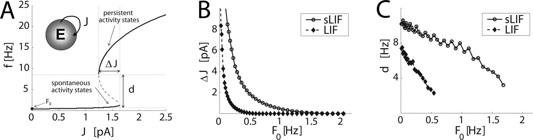
Divergent single-cell f–I curves increase the stability of persistent activity states emerging in recurrent random networks of IF model neurons. We compared populations of IF neurons with divergent f–I curves (sLIF) to populations of conventional leaky IF neurons (LIF). A , Existence and location of persistent states were studied as a bifurcation diagram, ΔJ denoting the range of J for which a spontaneous activity state and a persistent activity state simultaneously exist. d is the maximal width of the basin of attraction of the spontaneous activity state. In B and C , the robustness of the network bistability was studied by evaluating ΔJ and d as functions of F 0, which was regarded as a source of interference to the emergence or maintenance of network persistent states. In networks of sLIF neurons, the range of F 0 corresponding to two simultaneous equilibria was extended by ∼300% ( B , C ), and the sensitivity of d on F 0 (i.e., ∂d/∂F 0) was significantly reduced ( C ) compared with the performance of an identical network composed of LIF neurons. Model parameters are as follows: α = 0 pA s, τ m = 21.8 ms, C = 190.8 pF, H = −5.3 mV, τarp = 15.5 ms, and ω = 10.2 ms pA (sLIF) or ω = 0 ms pA (LIF).
Because no additional inhibitory population has been included in the model, the range ΔJ of such a recurrent excitatory coupling strength J is usually small (Fig. 8 A) and, together with the width d of the basin of attraction, shrinks as the level of spontaneous activity F 0 increases (Fig. 8 B,C). In Figure 8, we studied the range ΔJ and the width of the basin of attraction of stable solutions f* while increasing m 0 and s 0 to obtain an increase in the spontaneous activity F 0. Comparing identical networks of LIF (ω = 0) and sLIF (ω > 0) neurons required adjusting m 0 and s 0 in such a way that the same F 0 was achieved. When ΔJ and d were studied systematically as a function of F 0 , we found an ∼300% increase in the range of F 0 for which bistability exists when comparing sLIF neurons (ω > 0) to LIF neurons (ω = 0) (Fig. 8). Whereas for an infinitely large network, once a persistent state is reached, it will be retained endlessly, unless external perturbations occur, in small networks finite-size fluctuations might push the activity out of a persistent state when exceeding the width of the corresponding basin of attraction. This suggests that, in recurrent network of IF neurons with divergent f–I relationships, the emergence and maintenance of persistent states is generally more robust against fluctuations of background activity and heterogeneities of synaptic strengths.
Discussion
Comparison with previous work
To relate our results to previous observations obtained under similar conditions, we focused exclusively on current-clamp experiments and on a particular stimulation protocol, where the current mean m and SD s were separately manipulated (Rauch et al., 2003). Qualitative comparisons between different stimulation techniques require care, because different protocols may involve different definitions of noise input mean and SD. For example, Chance et al. (2002) reported a divergence in frequency-input curves in the SSC neurons (i.e., gain modulation) under dynamic clamp. That phenomenon, known as gain modulation, is unrelated to the divergence of the f–I curves (i.e., noise sensitivity plus mean insensitivity) observed here under current clamp. In fact, Chance et al. (2002) could account for the gain modulation by studying the theoretical response functions of conventional biophysical models as well as conductance-driven LIF neurons.
In our work, we aimed to unambiguously examine the suprathreshold regime and the effect of input fluctuations, characterizing the neuronal response for a large variety of inputs while not choosing any particular trajectory in the stimulation plane (m, s) (e.g., balanced excitation and inhibition). We studied the response regimes for relatively large values of m only to expose more clearly the difference in f–I curve sensitivity on s.
The peculiar response properties found here likely have been observed already in the SSC for a minority of cells. For example, Rauch et al. (2003) mention that they observed a divergence in the linear part of the f–I curves corresponding to distinct values of s, but L5 pyramidal cells could not usually sustain input currents stronger than 600–1000 pA for tens of seconds without substantial degeneration of the spike shape and a strong run down of the instantaneous firing rate. Depending on the cell type, a gain modulation by input noise has also been observed in the SSC (Higgs et al., 2006). Supporting our findings, Fellous et al. (2003) observed a qualitatively similar divergence of f–I curves in mPFC neurons by using the dynamic-clamp technique. However, reported absolute discharge frequencies and sensitivity to input fluctuations were markedly smaller than ours. In addition, their exclusive use of point-conductance injection technique makes it difficult to quantify the predominance of intrinsic membrane mechanisms, as isolated in our work, from effects associated to concomitant influences on the effective membrane time constants during stimulation.
In contrast, the f–I relationship of the mPFC neurons investigated here were characterized by unique and distinct saturation levels. The shift in spike threshold V th still was independent of s (Fig. 4 C), and it resulted in a delayed spike maximal upstroke velocity, without violating the stationarity criteria adopted by Rauch et al. (2003) (Fig. 1 C3, inset). Additionally, the input resistance and membrane capacitance of the mPFC cells clearly reflected a distinct population of layer 5 pyramidal neurons compared with the SSC cells analyzed (Rauch et al., 2003). Moreover, the response of mPFC neurons could not be fit by the LIF model routinely used for pyramidal neurons and interneurons in the SSC with success in previous reports (La Camera et al., 2006). Finally, both the plateau and the increased sensitivity to input fluctuations do not appear to be artifacts of long stimulation protocols, because they occur already within the first 2 s of stimulation (Fig. 3).
Concerning the suggested consequences of f–I curve divergence at the network level, we analyzed self-sustained stationary states emerging from networks where the local recurrent connectivity is mainly excitatory. Under these conditions, persistent states differ mainly in the mean current to the neurons (Amit and Brunel, 1997a). An alternative form of persistent states, driven by the fluctuations rather than by the mean of the input current to each neuron, has been described recently in recurrent networks of integrate-and-fire models, where excitation and inhibition strongly balance each other (Renart et al., 2007). Compared with the mean-driven persistent activity, fluctuation-driven states are determined by subthreshold input currents, require parameter fine-tuning, and have not been found to be a robust phenomenon (Renart et al., 2007). Because the divergence of the f–I relationships is a feature of the suprathreshold regime, we do not expect the stability of fluctuations-driven persistent states to be significantly enhanced in networks of sLIF neurons.
Implications for network information processing
What are the computational properties of mPFC pyramidal neurons? From the large variability in the distribution of ω, we suggest that two response profiles might exist in cortical pyramidal cells: (1) a substantially linear steady-state f–I profile, similar to that reported in the literature (Fig. 9 A), without sensitivity to fluctuations in the suprathreshold regime (i.e., above rheobase) (ω = 0 and small τarp); and (2) a saturating response function with increased sensitivity to the amount of fluctuations in the input (ω > 0 and large τarp) (Fig. 9 A). What happens when one interprets the consequence of such an observation in the context of simple models of internally generated activity in recurrent networks of excitatory and inhibitory model neurons (Amit and Brunel, 1997a; Vogels et al., 2005)?

Networks of model neurons compute either the SD or the mean of a global input during persistent activity. Excitatory IF neurons, alternatively characterized either as sLIF neurons with divergent f–I curves or as standard LIF neurons with convergent f–I curves, were assumed to be embedded into a larger pool of cells. The coexistence of an internally generated network state and of an external feedforward input i ext(t) was simplified by approximating the effect of i ext(t) as a modulation around two working points in the single neuron f–I curves (Eqs. 2, 3). For the sake of illustration, i ext(t) was a noisy waveform, characterized by a time-varying mean m(t) and a sinusoidally modulated variance s(t)2. The dotted blue line represents m(t), and the solid red lines represent m(t) ± s(t) (center inset). In the down state, the responses of the two networks are almost indistinguishable, whereas they significantly differ in the up state. In fact, in B , neurons exclusively propagate information encoded by m(t) (dashed line), whereas in D , they are strongly sensitive to s(t) (dashed line). Model parameters are as follows: A , best-fit response function as in Figure 8 C (left) of Rauch et al. (2003) (i.e., α = 5.3 pA s, τ m = 21.5 ms, C = 250 pF, H = 1.9 mV, and τarp = 4.2 ms, ω = 0); C , best-fit response function of a typical mPFC cell with similar effective membrane time constant (parameters as in Fig. 8); A , B , (m down, s down) = (100, 0) pA and (m up, s up) = (600, 50) pA; C , D , (m down, s down) = (21, 0) pA and (m up, s up) = (600, 50) pA.
To preliminary address this issue, we qualitatively studied the response of a homogeneous population of IF neurons assuming, for the sake of simplicity, that global persistence in two distinct network states was determined and maintained by an unmodelled recurrent network of excitatory and inhibitory neurons. We predict a differential and state-dependent feature extraction of an external input waveform i ext(t), globally fed into the excitatory neurons (Fig. 9). Intuitively, the shape of divergent f–I curves suggests that relatively high-rate spike trains contain relatively more information about input fluctuations s(t) than input mean m(t). Conversely, relatively high-rate spike trains from neurons with convergent f–I curves code m(t) more effectively than s(t). Indeed, as found in theoretical (Fourcaud-Trocmé et al., 2003) and experimental (H. Köndgen, C. Geilser, S. Fusi, X.-J. Wang, H.-R. Lüscher, and M. Giugliano, personal communication) work, when both m(t) and s(t) change slowly in time (i.e., <50–100 Hz), neuronal response properties are dominated by the f–I relationship and its local slope.
Figure 9 illustrates how two populations, characterized by distinct properties of single excitatory cells (Fig. 7 A–C) embedded in a large recurrent network, respond to a common foreground time-varying fluctuating input i ext(t). Each neuron of these networks receives a total current with mean and variance m tot = mean{i ext(t)} + m up/down and s tot = std{i ext(t)} + s up/down, where (m down, s down) and (m up, s up) are background input components set by the unmodelled network, and they correspond to the internally generated global persistent states. Although the two subnetworks are responding essentially in the same way during low-frequency spontaneous activity, because individual f–I curves differ only in the regime dominated by large values of m, they show differential computational properties as soon as they operate under a (self-sustained) higher frequency regime. In Figure 9, the distinct background network states have been referred to as up and down states, reminiscent of the literature suggesting that in vivo cortical networks might operate under distinct states (Holcman and Tsodyks, 2006) determined by the synaptic background activity (Destexhe et al., 2003; Salinas, 2003) and recently denoted as mean-driven (Renart et al., 2007).
By examining and comparing single-cell response profiles, it is natural to expect that in the downstates, the responses of the two networks are almost indistinguishable. However, the transformations performed by each neuron of the two networks differ significantly for the upstate. These networks exclusively propagate information coded in m(t) or in s(t) depending on their single-cell response profile but not both simultaneously as it occurs in the downstates. Then, one population would compute mean{i ext(t)} and the other std{i ext(t)}, as illustrated schematically in Figure 9, B and D.
Finally, another interesting prediction can be made for feedforward network architectures. To a first approximation, the mean of the overall synaptic input arising from the activity of Ne
excitatory and Ni
inhibitory afferent neurons firing asynchronously at fe
and fi
, respectively, is the difference between the excitatory and the inhibitory contributions [i.e., m = NeJefe
τ
e
− NiJifi
τ
i
, where τ
e
and τ
i
represent the decay time constant of individual synaptic events and Je
and Ji
represent the effective synaptic strength of the excitatory (e) and inhibitory (i) presynaptic afferents, respectively (Amit and Brunel, 1997a)]. Conversely, the variance of the inputs is the sum of individual variances (i.e., s
2 = 0.5 NeJe
2
fe
τ
e
+ 0.5 NiJi
2
fi
τ
i
) (Amit and Brunel, 1997a). Because individual neurons can exclusively encode information about their input mean or their input variance, ad-hoc postsynaptic read-out networks could recover and separate the information conveyed in the excitatory and inhibitory components. This would be the consequence of their selective response to the input mean or to the input variance, arising from converging or diverging f–I curves. In fact, fe
and fi
are related algebraically to m and s, being
 so that fe
∝ (2s
2 + mJi
), fi
∝ (2s
2 − mJe
).
so that fe
∝ (2s
2 + mJi
), fi
∝ (2s
2 − mJe
).
Therefore, simple dendritic and synaptic summation and subtraction (Poirazi et al., 2003a,b; Wolfart et al., 2005) might recover the distinct contributions fe (t) and fi (t) from the output of two neuronal populations, which process the same input but process it differently.
Relevance to previous and future studies
It has been proposed previously that neurons in primary sensory cortices quickly adapt to step changes in input fluctuations (Silberberg et al., 2004) and generally show low sensitivity to the input fluctuation, thereby maximizing the dynamical range of their response. For instance, Fairhall et al. (2001) discussed variance normalization in H1 cells of the fly visual system. This might contribute to a redundancy reduction in sensory systems (Buiatti and van Vreeswijk, 2003) and an efficient representation of sensory inputs (Dean et al., 2005). Similarly, spatial variance normalization has been reported as an adaptation strategy in V1 as well (Carandini et al., 1997), so that normalization of the temporal input variance might work equally well as a means of temporal contrast adaptation. Therefore, there may be computational constraints and requirements motivating why the response properties of SSC neurons show a steady-state insensitivity to input fluctuations.
In contrast, higher cortical areas might require different encoding strategies for associative and multisensory processing. The sensitivity to input fluctuations reported here might, for instance, constitute an additional candidate mechanism accounting for cross-modal response enhancement, similarly to what described in the deep layers of superior colliculus (Wallace et al., 1996). The response to one modality (i.e., input mean) might be augmented by another signal encoded as a different modality (i.e., input variance).
Following such a speculative view, no multiplicative mechanism (e.g., mediated by NMDAR) would need to be invoked in mPFC cortical networks. In addition, channel-specific enhancement or suppression could emerge from a change in the coherence of the activity in distinct converging synaptic pathways, resulting in a regulation of the amount of input fluctuations. In such a context, the emerging properties predicted in Figure 9 might effectively constitute a framework to interpret a modality/channel filtering, related to the actual network state.
In conclusion, data suggest that pyramidal neurons can compute in fundamentally different ways with regard to encoding information of input mean and variance in firing rate. An exhaustive in vitro characterization of the spike response properties of neurons from all layers, cell types, and cortex regions would be a first step toward a complete understanding of the information processing abilities possessed by individual cortical neurons.
Our approach has been that different computational capabilities of single neurons can translate into functionally distinct global populations of neurons. For instance, cortical interspike interval variability has been often reported to be large or unexpectedly low (Kara et al., 2000). This might be a specific indication of a distinct operational mode of individual neurons (e.g., whether they decode input fluctuations or respond to slower input components).
Similar to the investigation of Kara et al. (2000) from the retina to LGN and from LGN to V1, we envision future experimental attempts at characterizing how variability in the in vivo spike trains, coding for the same information, propagates centrally through higher cortical areas. The single-cell differential processing of input fluctuations revealed in the present study might provide a working framework to study and interpret the modulation of irregular firing in information propagation.
Finally, the impact of neuromodulatory systems on mechanisms for spike initiation, inactivation, and refractoriness might be studied in a novel context by examining resulting differences in single-cell coding strategies related to the encoding of input fluctuations.
Footnotes
-
This work was supported by Swiss National Science Foundation Grant 31-61335.00 (H.-R.L.), the Silva Casa Foundation, and Human Frontier Science Program Grant LT00561/2001-B (M.G.). B.N.L. was also supported by the Medical Scientist Training Program, a fellowship from the National Institute of General Medical Sciences (T32 07266), and an Achievement Rewards for College Scientists Foundation fellowship. We declare no conflict of interest. We thank Drs. S. Fusi, G. La Camera, A. Rauch, W. Senn, A. Fairhall, M. H. Higgs, and W. Spain for helpful discussions and Drs. A. Compte, N. Brunel, and K. Tseng for comments on this manuscript. B.N.L. and M.G. also thank Dr. K. Doya and the Okinawa Institute of Science and Technology for facilitating this collaboration.
- Correspondence should be addressed to Dr. Michele Giugliano, Ecole Polytechnique Fédérale de Lausanne, School of Life Sciences Brain Mind Institute Laboratory of Neural Microcircuitry, Station 15, CH-1015 Lausanne, Switzerland. michele.giugliano{at}epfl.ch


