

Abstract
Learning and memory formation in the brain depend on the plasticity of neural circuits. In the adult and developing cerebral cortex, this plasticity can result from the formation and elimination of dendritic spines. New synaptic contacts appear in the neuropil where the gaps between axonal and dendritic branches can be bridged by dendritic spines. Such sites are termed potential synapses. Here, we describe a theoretical framework for the analysis of spine remodeling plasticity. We provide a quantitative description of two models of spine remodeling in which the presence of a bouton is either required or not for the formation of a new synapse. We derive expressions for the density of potential synapses in the neuropil, the connectivity fraction, which is the ratio of actual to potential synapses, and the number of structurally different circuits attainable with spine remodeling. We calculate these parameters in mouse occipital cortex, rat CA1, monkey V1, and human temporal cortex. We find that, on average, a dendritic spine can choose among 4–7 potential targets in rodents and 10–20 potential targets in primates. The potential of neuropil for structural circuit remodeling is highest in rat CA1 (7.1–8.6 bits/μm3) and lowest in monkey V1 (1.3–1.5 bits/μm3). We also evaluate the lower bound of neuron selectivity in the choice of synaptic partners. Postsynaptic excitatory neurons in rodents make synaptic contacts with >21–30% of presynaptic axons encountered with new spine growth. Primate neurons appear to be more selective, making synaptic connections with >7–15% of encountered axons.
- filling fraction
- connectivity fraction
- potential synapse
- structural plasticity
- structural entropy
- spine length
Introduction
Many important brain functions such as learning and memory depend on the plasticity of neural circuits. Neurogeometric analysis of cortical neuropil shows that there are typically many axons within spine reach of a given dendrite (Stepanyants et al., 2002; Stepanyants and Chklovskii, 2005). Hence, cortical neuropil holds a potential for structural circuit reorganization through the retraction of some of the preexisting spines and the formation of new spines and synapses. This spine remodeling plasticity has a large capacity for modifying neural circuits (Stepanyants et al., 2002) and is thought to play an important role in learning and long-term memory formation (Chklovskii et al., 2004). There have been numerous in vivo experimental observations of spine remodeling plasticity in different cortical areas of developing and adult animals (Lendvai et al., 2000; Trachtenberg et al., 2002; Majewska and Sur, 2003; Holtmaat et al., 2005). Yet, it remains unclear how the new dendritic spines find their presynaptic targets and establish synaptic connections.
In this manuscript, we developed a theoretical framework that describes the capacity of cortical circuits to change with structural spine remodeling. We considered and compared two possible scenarios of structural plasticity: one where the initial synaptic contact can be made between a dendritic spine and a point on an axon, preceding bouton formation (Stepanyants et al., 2002), and the other where the initial synaptic contacts are preferentially established with preexisting synaptic boutons (Knott et al., 2006). Locations in the neuropil where synaptic contacts between axonal and dendritic branches can be made with new spine growth are termed potential synapses. Such axodendritic oppositions occur at different relative distances between neurites and, as a result, can be bridged by spines of different lengths. Hence, the shape of spine length distribution function is expected to reflect the potential of neuropil for spine remodeling. Longer spines can chose among a larger number of potentially presynaptic targets leading to a large number of possible circuits.
We calculated the density of potential synapses in the neuropil for the two quantitative models of spine remodeling plasticity. We derived an expression for the probability of an actual synapse being present at a potential synaptic site. This probability, or the connectivity fraction [formerly referred to as the filling fraction (Stepanyants et al., 2002)], was calculated as a function of distance between axonal and dendritic branches. We estimated the number of structurally different circuits that can be achieved by spine remodeling. This number, or structural synaptic entropy, is a measure of the potential of neuropil for circuit reorganization. Furthermore, we evaluated the selectivity of cortical neurons in their choice of synaptic partners. This selectivity, or probability for one neuron to establish a synaptic connection with another neuron encountered with a new spine growth, gives a sense of the number of functionally different classes of excitatory neurons in a small cortical region. Based on published anatomical data, we estimated and compared the above parameters of neuropil micro-architecture in mouse occipital cortex, rat CA1, monkey V1, and human temporal cortex. Our results showed marked differences in the potential for structural synaptic reorganization in these systems.
Materials and Methods
Models of structural synaptic plasticity
A potential synapse is a location in the neuropil where the distance s between an axon and a dendrite is small enough to be bridged by a dendritic spine (see Fig. 2A,B). We made this definition of a potential synapse more precise by considering the following two models. In model A (see Fig. 2C), we assumed that a spine can bridge the gap between the axon and the dendrite regardless of the presence of a bouton on the axon (Stepanyants et al., 2002; Stepanyants and Chklovskii, 2005). As a result, all dendrites that lay within the reach of a dendritic spine from the given axon are potential to that axon. In this model it was assumed that spine outgrowth and spine–axon contact precede bouton and synapse formation. In model B (see Fig. 2D), we assumed that the preexistence of a bouton on the axon is required for establishing a new synaptic connection (Kalisman et al., 2005; Knott et al., 2006). Hence, in this model, we defined a potential synapse as proximity between a bouton and a dendritic branch. In other words, all of the dendrites that lay within the reach of a dendritic spine from the given bouton are potential to that bouton.
Assumptions and approximations
Our method relies on several realistic assumptions and approximations. In the following we provide a list of assumptions specifying with A or B the model of potential connectivity for which these assumptions are needed.
We treated axonal (A) and dendritic (A, B) branches as straight segments on the scale of the average spine length (1–2 μm). This assumption holds for most excitatory neurons, including those in neocortex and hippocampus. It is justified by low tortuosity of dendritic and axonal branches of excitatory neurons on a micrometer scale (Stepanyants et al., 2004).
In calculating the numbers of potential synapses, we used an approximation where the average axonal (A) and dendritic (A, B) branch lengths were assumed to be much longer than the average spine length. Branch here was defined as a neuron process extending from soma or a bifurcation point to a successive bifurcation or an end point. This approximation ignores the corrections to the potential synapse count because of branch tips and bifurcation points. This approximation is certainly valid for the excitatory neurons in the cerebral cortex.
We made a simplifying assumption that axonal (A) and dendritic (A, B) branches of excitatory neurons are randomly distributed in the neuropil. Inhomogeneous distributions of branches would lead to spatial variations in the values of the calculated parameters. Yet, this should not affect the values averaged over large volumes of gray matter (e.g., 100 μm in size). This assumption is justified in part by the absence of short-range (1–2 μm) correlations between the positions of axonal and dendritic branches of neurons, i.e., axonal branches on average are not “attracted to” or “repelled from” dendrites (Stepanyants et al., 2004).
We assumed that synaptic contacts can occur anywhere along axonal (A) and dendritic (A, B) branches. In other words, there are no hot spots for spine and bouton formation. The presence of hot spots on dendritic branches would not change the results of our calculations because the average interspine interval is already smaller than the average spine length.
Although below in this section the results for model A are derived for an arbitrary distribution of angles between axonal and dendritic branches in the neuropil, in Results we make a simplifying assumption that this distribution is isotropic. This assumption had been verified (our unpublished data) on the dataset of cortical excitatory neurons reconstructed in three dimensions (Stepanyants et al., 2008). It is already valid if the orientations of either axonal or dendritic branches are isotropic. Anisotropic distribution of angles could lead to a slightly different numerical coefficient in Equations 12 and 13 (see below).
In Results, we make a simplifying approximation in which the number of asymmetric synapses is approximately equal to the number of boutons on excitatory neuron axons (A, B). This is because the majority of boutons on excitatory axons contain only a single asymmetric synapse. This approximation is supported by low fractions of multiple synapse boutons: 0.026 in cat primary visual cortex (Kisvárday et al., 1986; Anderson et al., 1994), 0.16 in rat motor cortex (Jones, 1999), 0.18–0.24 in rat hippocampus (Sorra and Harris, 1993; Yankova et al., 2001), and 0.14 in mouse barrel cortex (Knott et al., 2006). The average asymmetric synapse to bouton ratio is 1.08 in mouse neocortex (Braitenberg and Schüz, 1998). For asymmetric synapse to bouton ratios much larger than one, it would be necessary to use more precise expressions (Eq. 8).
Another simplifying approximation made in Results is that the volume density of spines of excitatory neuron dendrites is equal to the volume density of asymmetric synapses (A, B). This approximation is supported by generally low fractions of asymmetric synapses that are not made on dendritic spines of excitatory neurons. For example, in mouse neocortex, this fraction is estimated at 0.13 (Braitenberg and Schüz, 1998). For large fractions of such synapses, it would be necessary to use Equation 11 (see below).
We did not take into consideration volume exclusion effects in the neuropil (A, B), assuming that neurites are flexible and can be easily deformed to accommodate synaptic connections. Such effects could be important near the dendritic shafts where the space is partly occupied by inhibitory axons and their shaft synapses. This may effectively push the excitatory axons farther out. Hence, our results may not be accurate for small values of the parameter s (<0.5 μm).
We assumed that dendritic spines are straight segments that extend perpendicularly to the dendritic shafts (A, B). In model A, we made an additional assumption that dendritic spines bridge the gaps between potentially connected axons and dendrites along the shortest paths. Thus, in this model, a spine connecting an axon and a dendrite is perpendicular to both branches. We address these limitations of our models in Discussion.
Optical measurements of spine length distribution functions may not be accurate. First, because of the limited resolution, spine lengths shorter than 0.5 μm cannot be measured accurately. Second, some dendritic spines can be overshadowed by the dendrite. Third, spines that do not lie entirely in the focal plane will appear shorter, shifting the spine length distribution function to the left. In the experimental data used in this study, the last two effects were minimized by only measuring spines which lie in the focal plane on both sides of the dendritic branch.
Volume density of potential synapses
In the following, we calculate the density of potential synapses in the neuropil. We begin by calculating the probability PA(d) that two long straight segments of given orientations (making angle θ with each other) and lengths la and ld (la,d ≫ d), randomly positioned inside a large volume V, will be within distance d of each other (Fig. 1A). Clearly, the two segments are located within distance d of each other if one segment penetrates the imaginary cylinder of radius d surrounding the other segment. The probability of this event is equal to the probability for the origin of the first segment to fall inside the right prism (2d by la by ld and angle θ at the base) as shown in Figure 1A. Hence, PA(d) is equal to the ratio of the volume of the prism and volume V:
 Similarly, one can calculate the probability PB(d) that a long straight segment of a given orientation and length ld, randomly positioned inside a large volume V, will be located within distance d of a given point (Fig. 1B). The segment is located within distance d of the point if it intersects an imaginary sphere of radius d centered at the point. The probability of this event is equal to the probability for the origin of the segment to be located inside the cylinder of radius d and length ld as shown in Figure 1B. As a result, PB(d) is equal to the ratio of the volume of the cylinder and volume V:
 Now, consider a straight axonal segment of length lai and radius ra located inside a large neuropil volume V (model A). A randomly chosen dendritic segment of length ldj, radius rd, and a given orientation in the neuropil (making an angle θij with the axon) makes a potential synapse that can be bridged by a spine in the [0, s] length range, if the axis of this segment is located within distance d from the axis of the axon, such that ra + rd ≤ d ≤ s + ra + rd. This means that the surfaces of the axonal and dendritic cylinders must be closer than a distance s without touching each other. The probability of this happening is equal to the difference of probabilities PijA(s + ra + rd) − PijA(ra + rd), where subscripts are added in reference to segments i and j. In model B, a dendritic segment and a bouton of radius rb can be bridged by a spine in the [0, s] length range if the axis of the dendritic segment is located within distance d from the center of the bouton, such that rb + rd ≤ d ≤ s + rb + rd. As a result, the probability of potential connection is PijB(s + rb + rd) − PijB(rb + rd).

Probability of potential connection for line segments. A, The probability that a random line segment of a given orientation and length ld (black) is located within distance d from another segment (gray) of length la (la,d ≫ d) is equal to the probability that the origin of the first segment falls inside the prism shown in the figure. B, The probability that a random line segment (black) of length ld is located within distance d from a given point (gray dot) is equal to the probability that the origin of this segment falls inside the cylinder of length ld and radius d as shown.
Using Equations 1 and 2 for models A and B, respectively, the probabilities of potential connection corresponding to spine lengths in the [0, s] range reduce to the following:
 In the second equation, δ = rd + rb is the sum of dendritic and bouton radii (Table 1). The expected cumulative number of potential synapses in the neuropil volume V that can be bridged by spines shorter than s is the sum of the probabilities in Equation 3 over all of the dendritic segments (i) and potentially postsynaptic elements (j, axonal segments in model A or boutons in model B):
 Because of the assumption of no correlation in the layout of axonal and dendritic branches, the sum in the first equation breaks down into a product of axonal and dendritic components. As a result, the cumulative number of potential synapses reduces to the following:
 In these expressions, La and Ld are the combined axonal and dendritic lengths, Nb is the total number of boutons in the neuropil volume V, and s̅i̅n̅θ̅ is the average sine of angles between axonal and dendritic branches.
Anatomical parameters of synaptic circuits from mouse, rat, monkey, and human cortexes
Because La, Ld, Nb, and the cumulative number of potential synapses NpotA,B(s) are intensive quantities of volume, Equation 5 can be conveniently rewritten in terms of densities:
 where ρa,d are the axonal and dendritic length densities (combined length of axons or dendrites in a unit volume of neuropil) and nb denotes the volume density of boutons. If relative orientations of axonal and dendritic branches are isotropically distributed (which is already true if either axonal or dendritic branches are isotropic), s̅i̅n̅θ̅ = π/4 (Stepanyants et al., 2002). This simplification is used in Results. Note that models A and B result in different dependence of the cumulative potential synapse density on spine length s.
The connectivity fraction
The probability of finding an actual synaptic connection at a potential synaptic site is described by the connectivity fraction of neuropil, f. The connectivity fraction is a measure of plasticity potential associated with spine remodeling. It reflects the number of structurally different circuits that can be realized in a given neuropil volume through spine reorganization. As the cumulative number of potential synapses depends on distance s, the connectivity fraction, in general, will be dependent on s as well, f(s).
To calculate fA,B(s), we note that in a unit volume of neuropil there are Δnact(s) = nspinep(s)Δs actual synapses on spines in the [s − Δs/2, s + Δs/2] length range. Here, p(s) is the spine length distribution function and nspine is the volume density of spines. These Δnact(s) spines are distributed among ΔnpotA,B(s) potential synaptic sites (derived from Eq. 6). The connectivity fraction fA,B(s) can be obtained as the ratio of the numbers of spines and potential synapses in the [s − Δs/2, s + Δs/2] interval:
 The above expressions are not convenient for making quantitative estimates of the connectivity fraction. This is because axonal and dendritic length densities are not typically measured in experiments. To get around this problem, we note that the ratio nspine/ρd is equal to the average linear density of spines on the excitatory neuron dendrites, or the inverse of the interspine interval on a dendrite, 1/bd. Similarly, ρa can be expressed as the product of the average interbouton interval on the excitatory neuron axons, ba, and volume density of these boutons, nb (ρa = banb). Finally, denoting the ratio between the number of asymmetric synapses, ns, and the number of boutons, nb, on excitatory neuron axons as m (ns = nbm), we arrive at the final expressions for the connectivity fractions in models A and B:
 All of the components in these expressions are routinely measured with electron or light microscopy. For convenience, in Equation 8 we broke down the connectivity fractions into a product of two parts: dimensionless parameters fA,B*, which depend on the anatomical details of neuropil organization, and a dimensionless part which is primarily dependent on the shape of the spine length distribution function. In Results, Equation 8 appears with the values of m = 1 mt s̅i̅n̅θ̅ = π/4 (see Assumptions and approximation).
A parameter similar to fA* was initially introduced in Stepanyants et al. (2002) under the name of filling fraction. One difference being that in our earlier work spine length was measured between the tip of the spine head and the dendritic axis as opposed to the base of the spine. The value of this dimensionless parameter was estimated to be in the 0.1–0.3 range for many species and cortical areas consistent with the results of this study.
Structural synaptic entropy of circuits in the neuropil
Next, we calculate the structural entropy associated with possible connectivity patterns in the neuropil which can be attained with spine remodeling. This entropy can be viewed as the potential of neuropil to form different circuits. It is important to note that structurally different connectivity patterns in terms of individual synapses do not necessarily correspond to functionally different circuits at the level of individual neurons. For example, an axonal arbor of a presynaptic excitatory neuron in the neocortex typically makes several potential synapses with a dendritic arbor of a neighboring excitatory postsynaptic cell (Stepanyants et al., 2008). It is quite possible that different choices of actual synapses out of the potential ones do not result in functionally different connections between the two cells. Hence, the structural synaptic entropy only provides the upper bound of (but may be correlated with) the number of functionally different circuits that can be attained with structural spine remodeling.
The neuropil volume V contains ΔnpotA,BV potential and ΔnactV actual synapses in the [s − Δs/2, s + Δs/2] range of spine lengths. In this range, the number of ways to choose actual synapses out of the pool of potential ones is given by the following binomial coefficient:
 The structural synaptic entropy, ΔIA,B(s), is defined as the log2 of this number. In the limit of large numbers of actual and potential synapses (large V), the binomial coefficient can be approximated using Stirling's formula (Arfken and Weber, 2005), and
 In this expression, iA,B(s) is referred to as entropy density distribution.
Because the structural synaptic entropy, ΔIA,B(s), is proportional to the volume of neuropil, it is natural to introduce the volume density of this quantity. Adding the entropic contributions arising from different spine length intervals, Δs, we obtain the overall structural synaptic entropy per volume of neuropil:
 Model dependence in this expression is contained in the connectivity fraction f(s) (Eq. 8). The structural synaptic entropy per volume scales with the volume density of spines, nspine. It is a functional of the spine length distribution function p(s) and depends on anatomical characteristics of neuropil microarchitecture through nspine, ns, ba, bd, and m. In Results, we use a simplified version of Equation 11, where the volume density of spines, nspine, is replaced with the volume density of asymmetric synapses, ns (see above, Assumptions and approximations).
Estimation of error bars
In this study, we compared parameters of structural synaptic plasticity in different systems. Such comparisons are hindered by generally large variability in anatomical measurements, and significant differences (if any) can only be observed on the level of the mean values. Hence, it is necessary to provide quantitative estimates of the SEMs. Because the raw experimental data for the studies cited in Table 1 were not available to us, our strategy here was to estimate the upper bounds of the SEMs from the reported SDs and the numbers of measurements.
Consider an experiment where a statistical measurement is performed in n brains from multiple samples per brain. The samples are then pooled together and the mean and total variance (var = SD2) are reported as results of the experiment. Table 1 shows a number of such experiments where the interbouton interval along an axon, the spine density on a dendrite, and the density of asymmetric synapses in different systems were measured. To access interbrain variability, we would like to estimate the variance in the average measurements for different brains. For this, we note that the total variance is equal to the sum of the average within-brain variance and variance in the averages for different brains. Hence, variance in the averages for different brains is always less or equal to the total variance. Then, the upper bound of the SE to the mean is equal to the square root of the total variance divided by n,
When calculating the product of two or more measured variables, we propagated their SEMs using the Monte Carlo procedure. Here, we took advantage of the central limit theorem (Arfken and Weber, 2005) and for each variable generated a set of 10,000 elements from a Gaussian distribution with the measured mean value and the SEM estimated as described above. Next, we calculated the product between all members of the sets and obtained the mean and the SEM for the product. This is how the mean and the SEM values were estimated for all of the calculated quantities, including the dendritic length density ρd from Table 1 and all of the parameters from Table 2. To test for the pairwise difference in the means of the calculated parameters and to obtain the corresponding p values, we used the Student's t test for samples with unequal variance.
Parameters of structural circuit remodeling in mouse, rat, monkey, and human cortexes
Anatomical data
To evaluate the connectivity fraction and the capacity of neural circuits to undergo structural remodeling, we used previously published anatomical data from some of the best-studied cortical systems. Our choice of the cortical systems was primarily restricted by the availability of the spine length distribution function and we confined our analysis to mouse occipital cortex, rat CA1, monkey V1, and human temporal cortex. The anatomical parameters of circuit microarchitecture in these areas are provided in Table 1. Below we give a detailed account of how these parameters were selected. Unless stated otherwise, the numerical values are shown as mean ± SD (SEM).
Mouse occipital cortex.
Anatomical data for the mouse occipital cortex was based on measurements from adult mice. The distributions of spine neck lengths and spine head areas were measured on basal dendrites of layer 3 pyramidal cells of two mice (Benavides-Piccione et al., 2002). Because there is no correlation between spine neck length and spine head area (Benavides-Piccione et al., 2002), these distributions were used to generate the spine length (neck length plus head diameter) distribution. This was done with the following Monte Carlo procedure. Ten thousand spine neck lengths and head areas were sampled from their corresponding distributions. The average spine head diameters were calculated for each spine head. These diameters were randomly associated with different spine neck lengths to generate the spine length distribution function (see Fig. 3A1). The average spine length obtained from this distribution was 0.99 ± (0.01) μm (n = 2 mice, 1226 spines). The correction for hidden spines (spines above and below the dendrite) was deemed unnecessary, as only lateral spines were reconstructed in the above study. Parameter δ was estimated at 0.70 μm, which is the sum of the average radius of dendritic branches, 0.45 μm (Braitenberg and Schüz, 1998), and the average radius of synaptic boutons, 0.25 μm (Braitenberg and Schüz, 1998). Although, this value of the parameter δ was based on several cortical regions and does not contain error bars, it does not affect strongly the results of our theory. This parameter is only present in model B, Equation 8, and has only an effect on our results in the region of small spine lengths. The average interbouton interval was estimated to be 4.5 ± 1.4 (0.47) μm (n = 9 mice, 20 cells) based on measurements in layers 2–4 of different cortical areas (Schüz and Palm, 1989; Hellwig et al., 1994; Braitenberg and Schüz, 1998). Because no significant variations in ba between cortical areas is reported (Hellwig et al., 1994), we used this value to represent the interbouton interval in the mouse occipital cortex. Based on (Schüz, 1976; Braitenberg and Schüz, 1998) the average spine density along a dendrite, 1/bd, is 1.94 ± 0.42 (0.24) μm−1 (n = 3 mice, 10 cells). The volume density of asymmetric synapses in layer 3 of mouse occipital cortex is 0.91 ± 0.25 (0.15) μm−3 (n = 3 mice, 3 blocks of tissue). This value was calculated as the product of the total synapse density, 1.05 ± 0.29 (0.17) μm−3, and the 0.87 fraction of asymmetric synapses (Schüz and Palm, 1989; Braitenberg and Schüz, 1998). We would like to mention that a significantly higher estimate of the average density of asymmetric synapses, 2.2 μm−3 (n = 1 mouse), was reported by DeFelipe et al. (2002). We did not use this measurement because it is based on a single animal and is averaged across all cortical layers. However, the discrepancy in the densities of asymmetric synapses may have resulted from methodological differences. This point is further addressed in the discussion section. The dendritic length density calculated as the product of the interspine interval and the density of asymmetric synapses is 0.48 ± (0.10) μm−2, implying that one cubic micrometer of neuropil in layer 3 of adult mouse occipital cortex contains on average 0.48 μm of dendritic length.
Rat CA1.
Anatomical data for the rat hippocampus was based on measurements in stratum radiatum of CA1 region in adult Long–Evans and Wistar rats. Here, the spine length distribution function (see Fig. 3A2) was derived from the work of Petrak et al. (2005) (n = 2 rats, 485 spines). In this work the cumulative distribution is scaled to the median spine length of 1 μm. Hence, in generating the distribution in Figure 3A2 we differentiated the original cumulative distribution and rescaled it to the average spine length of 1.08 ± (0.03) μm (n = 4 rats, 351 spines). This value of spine length was determined by averaging the results from the studies by Harris and Stevens (1989) [0.95 ± 0.42 μm (n = 3 rats, 100 spines)] and Trommald et al. (1995) [1.21 ± 0.43 μm (n = 1 rats, 251 spines)]. The value of the average radius of dendritic branches in stratum radiatum, 0.30 μm, was obtained by averaging the results from the studies by Harris and Stevens (1989) [0.28 μm (n = 3 rats, 7 dendritic segments)], Trommald et al. (1995) [0.36 μm (n = 3 rats, 3 cells)], and Megías et al. (2001) [0.25 μm (n = 7 rats, 26 dendritic segments)]. This value was added to the average radius of synaptic boutons, 0.2 μm (n = 2 rats, 224 varicosities) (Shepherd and Harris, 1998), resulting in δ = 0.5 μm. The average interbouton interval in stratum radiatum of rat CA1, 3.7 ± 0.6 (0.3) μm (n = 5 rats, 1909 varicosities), was based on measurements for CA3 axons projecting to CA1 (Shepherd et al., 2002). This value of interbouton interval is consistent with the value of 3.0 ± 1.4 μm reported by Shepherd and Harris (1998), which has to be corrected for tissue shrinkage by an estimated 10–25% (Shepherd and Harris, 1998). The density of spines on a dendrite, 1/bd, in stratum radiatum of rat CA1, 3.41 ± 1.05 (0.40) μm−1 (n = 7 rats, 20 cells), was obtained from the work of Megías et al. (2001). This value is approximately in the middle between the two other reported measurements of spine density, 3.03 ± 0.83 (0.59) μm−1 (n = 2 rats, 15 dendrites) (Harris et al., 1992) and 3.80 ± 0.76 (0.54) μm−1 (n = 2 rats, 26 dendrites) (Petrak et al., 2005). Pooling all of the data together would not result in a significant change in the density of spines. Using the density of asymmetric synapses of 2.0 ± 0.30 (0.13) μm−3 (n = 5 rats, 5 blocks of tissue) (Sorra et al., 1998), we estimated that the dendritic length density in stratum radiatum of rat CA1 is 0.59 ± (0.08) μm−2. This result is similar to that in the mouse occipital cortex.
Monkey V1.
These data were based on measurements from layer 3 of adult Macaque monkey primary visual cortex. Here, the distribution of spine lengths on basal dendrites was obtained from the work of Stepanyants et al. (2002), where the spine length was measured between a point on the dendritic axis closest to the base of the spine and the tip of the spine head. As in the present work, spine length was measured from the dendritic surface, the original distribution was shifted to the left by 0.70 μm, the amount corresponding to the average radius of basal dendrites (Stepanyants et al., 2002). The resulting distribution (see Fig. 3A3) has the average spine length of 1.86 ± (0.05) μm (n = 3 monkeys, 233 spines). Parameter δ was estimated as the sum of the average radius of basal dendritic branches, 0.70 μm, and the generic average radius of synaptic boutons, 0.25 μm. As stated above, this parameter does not strongly affect the results of our calculations. We obtained the average interbouton interval in layer 3 of monkey V1 from the work of Amir et al. (1993). The interbouton histogram in this study is consistent with an average interbouton interval of 5.6 ± 2.4 (1.2) μm (n = 4 monkeys, 400 varicosities) reported as 180 boutons/mm. To estimate the average spine density on basal dendrites we pooled together data from four different studies (Elston and Rosa, 1997, 1998; Elston et al., 1999, 2005) performed in Macaque primary visual cortex. Our estimate of 1/bd, which was based on the reported measurements of spine density and the number of branches as a function of distance from soma, resulted in 0.55 ± 0.07 (0.03) μm−1 (n = 5 monkeys). The volume density of asymmetric synapses was calculated as the product of the volume density of all synapses in layer 3 of adult Macaque monkey V1, 0.34 ± 0.04 (0.02) μm−3 (n = 3 monkeys, 9 blocks of tissue) (O'Kusky and Colonnier, 1982), and the fraction of asymmetric synapses, 0.76 ± 0.09 (0.06) (n = 2 monkeys, 5 blocks of tissue) (Bourgeois and Rakic, 1993), resulting in 0.26 ± 0.04 (0.03) μm−3. This estimate led to the average dendritic length density of 0.47 ± (0.05) μm−2.
Human temporal cortex.
The spine length distribution function was derived from the work of Benavides-Piccione et al. (2002). Here, the distributions of spine neck lengths and spine head areas were measured on basal dendrites of layer 3 pyramidal cells in temporal cortexes of two adult male patients. The spine length distribution (see Fig. 3A4) was generated in the same way as for mouse occipital cortex, resulting in the average spine length of 1.42 ± (0.01) μm (n = 2 humans, 2768 spines). The value of parameter δ, which in this case is equal to the sum of the average radii of second order dendritic branches and synaptic boutons, was estimated as 1.1 μm + 0.25 μm. The former number was based on the analysis of published neuron images (Benavides-Piccione et al., 2002) and the latter is the generic value of the average bouton radius. We did not find a reliable estimate of the average interbouton interval in human temporal cortex and, thus, we provided results for model B only. The value of the average spine density on basal dendrites of layer 3 pyramidal cells in human temporal cortex, 2.62 μm−1 (n = 1 human, 73 dendrites), comes from the work of Elston et al. (2001). This type of data is very difficult to come by, and in this study we used measurements from only a single human subject. We did not use the measurements of the spine density reported by Benavides-Piccione et al. (2002) for two human patients because in that comparative study no correction was made for hidden spines, i.e., spines located directly above or below the dendrite. To have an estimate of the extent of intersubject variability, we applied the variability observed in the monkey spine density to the human data. This estimate is justified in part by the fact that a similar coefficient of variation had been observed in human data from the study by Benavides-Piccione et al. (2002). This resulted in a spine density of 2.62 ± 0.34 (0.34) μm−1. The volume density of asymmetric synapses in layer 3 of human temporal cortex was calculated by multiplying the density of all synapses with the reported fraction of asymmetric synapses resulting in 1.07 ± 0.31(0.18) μm−3 (n = 3 humans, 60 blocks of tissue) (DeFelipe et al., 2002). As a result, the dendritic length density calculated as the product of the interspine interval and the density of asymmetric synapses was 0.42 ± (0.09) μm−2.
Results
Below, we describe the theoretical framework of structural spine remodeling. Our numerical results were based on the analysis of previously published anatomical data from mouse occipital cortex, rat CA1, monkey V1, and human temporal cortex (Table 1). The experimentally measured spine length distributions in these areas are shown in Figures 3A. Based on the shapes of the spine length distributions and average anatomical parameters, we evaluated and compared the potential of neuropil for structural plasticity in these systems.
Potential synapse
A potential synapse is a location in the neuropil where the distance s between an axon and a dendrite is small enough to be bridged by a dendritic spine (Fig. 2A,B). Model A (Fig. 2C) further assumes that such axon–dendrite oppositions can be converted into synaptic connections by dendritic spines, regardless of the presence of boutons on the axons (Stepanyants et al., 2002; Stepanyants and Chklovskii, 2005). As a result, all of the dendrites that lay within dendritic spine reach from a given axon are potential to that axon. In this model, it was assumed that spine outgrowth and spine–axon contact precedes bouton and synapse formation. Of course, some spines can by chance make contacts with preexisting boutons, leading to the formation of multiple synapse boutons. There is however some direct and indirect experimental evidence that the presence of a bouton on an axon is required for establishing a new synaptic connection (Kalisman et al., 2005; Knott et al., 2006). Hence, in model B we defined a potential synapse as a proximity between a bouton and a dendritic branch (Fig. 2D). In other words, all of the dendrites that lay within spine reach from a given bouton are potential to that bouton.

Potential synapse. A, Three-dimensional reconstructions of a layer 4 spiny stellate cell axon (blue) and a layer 3 pyramidal cell dendrite (red) from the cat primary visual cortex. Potential synapses between the arbors are shown with small black circles. Scale bar, 100 μm [modified from Stepanyants et al. (2008), their Fig. 4]. B, Schematic illustration of a 5 × 5 × 5 μm volume of cortical neuropil (based on the data from mouse occipital cortex) (Table 1). The axonal and dendritic segments shown are potentially connected if they can be bridged by dendritic spines. Densities of axons and dendrites were reduced sixfold to avoid clutter. C, D, Two models of potential connectivity. In C, a potential synapse is defined as a site in the neuropil where a dendritic branch is located a distance s away from an axon (model A). Presence of a synaptic bouton on the axon is not required. In D (model B), a potential synapse is defined as a location in the neuropil where a dendritic branch is present a distance s away from an existing synaptic bouton (blue sphere on the axon).
Density of potential synapses
Because dendritic spines come in a range of lengths (Fig. 3A1–A4), the number of potential synapses is dependent on the spine length. In a volume of neuropil the cumulative density of potential synapses for a given spine length s includes all axon–dendrite oppositions that can be bridged by dendritic spines shorter than s. This number depends on the densities of axonal and dendritic branches in the neuropil volume and the model of synaptogenesis.

Characterization of structural spine remodeling. A1–A4, Spine length distributions: mouse occipital cortex (A1), area CA1 of rat hippocampus (A2), monkey visual area V1 (A3), and human temporal cortex (A4). B1–B4, Connectivity fraction as a function of spine length. The connectivity fraction is the ratio of the numbers of actual to potential synapses. Results based on model A are shown with black dashed lines and those based on model B are shown with gray solid lines. C1–C4, Structural entropy density per spine as a function of spine length. The overall structural entropy per spine can be calculated as the area under the curves. Error bars indicate SEM.
In model A, a potential synapse was defined symmetrically with respect to axonal and dendritic branches (Fig. 2C). As a result, the cumulative density of potential synapses in the neuropil, npotA (s), depends on the product of axonal and dendritic length densities, ρa and ρd, of excitatory neurons. Length density is the combined length of neurites (axons or dendrites) in a unit volume of neuropil. In model B (Fig. 2D), a potential synapse was defined as an opposition between a bouton and a dendrite, and, thus, npotB (s) depends on the product of the volume density of boutons, nb, and the dendritic length density. Detailed derivation of the volume densities of potential synapses is provided in Materials and Methods, where the following expressions were derived for models A and B, respectively:
 In the last expression, δ is the sum of the average dendritic and bouton radii. Note that in model A the cumulative density of potential synapses depends linearly on the spine length s, whereas in model B the dependence is quadratic. Because the majority of excitatory synapses are made on dendritic spines (Kisvárday et al., 1986) and the majority of spines bear a single excitatory synapse, the dendritic length density can be estimated as the product of the asymmetric synapse density and the average interspine interval along excitatory dendrites, ρd ≈ nsbd. The estimated values of ρd for the four considered systems are shown in Table 1. Similarly, the axonal length density can be estimated as the product of the density of asymmetric synapses and the average interbouton interval on excitatory neuron axons, ρa ≈ nsba. Because of the presence of multiple synapse boutons, this expression may slightly overestimate the axonal length density (for more detailed expressions, see Materials and Methods).
Connectivity fraction
To evaluate the potential of cortical neuropil for structural circuit reorganization by spine remodeling, we introduced the connectivity fraction, fA,B(s), which was defined as the ratio of the numbers of spines and potential synapses in the [s − Δs/2, s + Δs/2] length interval. In other words, the connectivity fraction is the fraction of potential synapses (for a given spine length, s) which had been converted into actual ones. According to this definition, fA,B(s) ≤ 1 for all values of s. Calculation details of the connectivity fraction in models A and B are provided in Materials and Methods. The connectivity fraction depends on the shape of the spine length distribution function, p (s), as well as average anatomical parameters of cortical microarchitecture (Table 1). The latter dependence is mainly captured by a single parameter fA,B*, which is referred to as the connectivity parameter (Table 2):
 We evaluated the expressions for the connectivity fraction based on the experimentally measured spine length distribution functions and the values of anatomical parameters (Table 1) for the four considered cortical areas. The results for models A and B are shown in Figure 3B1–B4 and Table 2. As was expected from the definition of the connectivity fraction, f(s) ≤ 1 for all values of s in all numerical results.
The most salient feature of the results in Figure 3B1–B4 is that the average (or peak, fmax) connectivity fractions, −f, in rodents are significantly higher than those in the primates (p < 0.05 for all pairwise comparisons, Student's t test for samples with unequal variance). There are no significant differences in −f within rodent and primate groups. For example, in mouse occipital cortex the average connectivity fraction is 0.19 for model A (see Table 2) indicating that on average a spine can choose among approximately five potentially presynaptic axons. For model B, f̄ = 0.14, which means that a single bouton can be contacted by approximately seven potentially postsynaptic dendrites. In contrast, the average connectivity fraction in human temporal cortex is 0.072 in model B, which is significantly smaller (p < 0.03). Here, a single bouton can be contacted by an astounding 14 different postsynaptic dendritic spines.
Capacity of cortical circuits for structural remodeling
The number of structurally different circuits attainable by remodeling of dendritic spines of length s is described by the structural entropy density per spine, iA,B (s)/ns (for details, see Materials and Methods).
 The results of calculations based on this expression are shown in Figure 3C1–C4. The shapes of the entropy density curves approximately follow the shapes of the spine length distribution functions. For large values of spine length, s, the entropy density per spine in model B is larger than that in model A. This trend, which is exactly opposite to the trend in the connectivity fractions shown in Figure 3B1–B4, is attributable to the fact that large connectivity fractions correspond to low entropy densities per spine and vice versa (Eq. 14, Fig. 5). In mouse occipital cortex, the structural entropy density per spine peaks at approximately 3bits/μm for 1 μm spines. This means that, for example, spines in the range of lengths from 0.95 to 1.05 μm contribute 3 bits/μm × 0.1 μm = 0.3 bits of entropy per spine to structural connectivity. The peak entropy density per spine is highest in rat CA1, 3.0 bits/μm in model A and 3.7 bits/μm in model B.
Integrating Equation 14 over spine lengths (Fig. 3C1–C4, areas under the curves), we arrived at the expression for the overall structural entropy per dendritic spine:
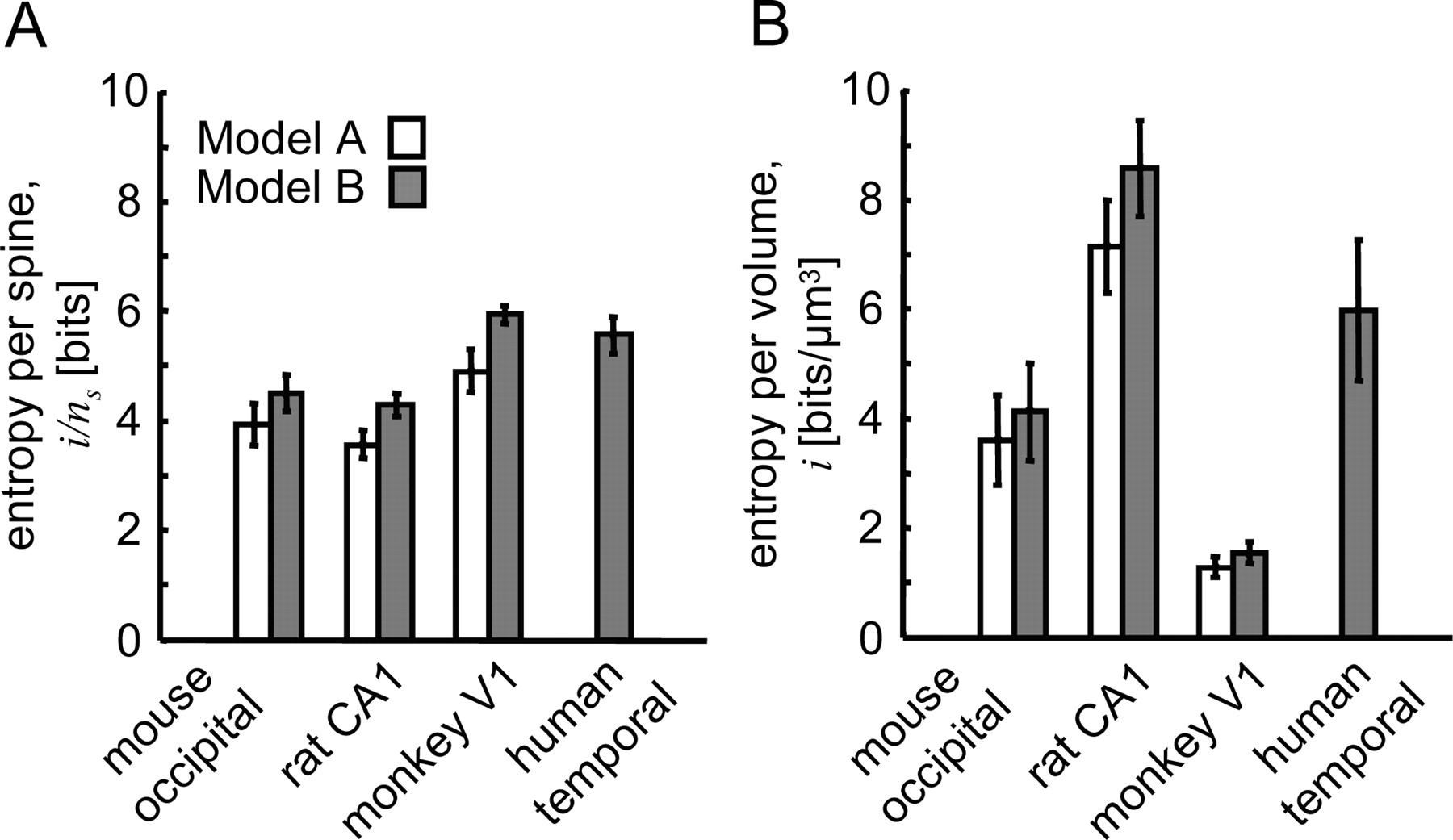
 The results of this calculation are shown in Figure 4A and Table 2. In rodent cortex, a single spine can contribute 3.6–4.5 bits of entropy to the patterns of synaptic connectivity. In monkey V1 and human temporal cortex, the amount of entropy available to a single spine is significantly higher, 4.9–5.9 bits (p < 0.04 for all pairwise comparisons). In addition, we did not detect any significant differences in structural entropy per spine within rodent and primate groups. The fact that a single spine in primate cortex has high entropy for structural plasticity seems satisfactory. Yet, in comparison, low entropy per spine (3.6–4.3 bits) in the rat CA1, an essential learning and memory area, could seem surprising. However, this lack of structural entropy per spine in rat CA1 is compensated by a large density of synapses.

Potential for structural plasticity. A, Structural entropy per spine in mouse occipital cortex, rat CA1, monkey V1, and human temporal cortex. White bars show the results based on model A and gray bars correspond to model B. B, Structural entropy per volume of cortical neuropil. Error bars indicate SEM.
Multiplying the entropy per spine, iA,B/ns, with the density of asymmetric synapses, ns, we obtain the structural synaptic entropy per volume of neuropil, iA,B (see Fig. 4B, Table 2). This quantity reflects the number of structurally different circuits that can be achieved with spine remodeling in the unit volume of cortical neuropil. With the exception of comparison between mouse and human in model B, all within-model differences in Figure 4B are significant (p < 0.05). Structural entropy per volume is highest in the rat CA1, 7.1–8.6 bits/μm3, and lowest in the monkey V1, 1.3–1.5 bits/μm3, primarily because of the high and low densities of asymmetric synapses in these cortical areas.
The average structural entropy per spine, iA,B/ns, according to Equations 13 and 14, depends only on the shape of the spine length distribution function p (s) and the connectivity parameter fA,B*. Figure 5 shows the dependence of iA,B/ns on fA,B* in models A and B. The dots indicate the results of the calculations based on the data from Tables 1 and 2. For a given spine length distribution function, the structural entropy per spine is a decreasing function of the connectivity parameter.
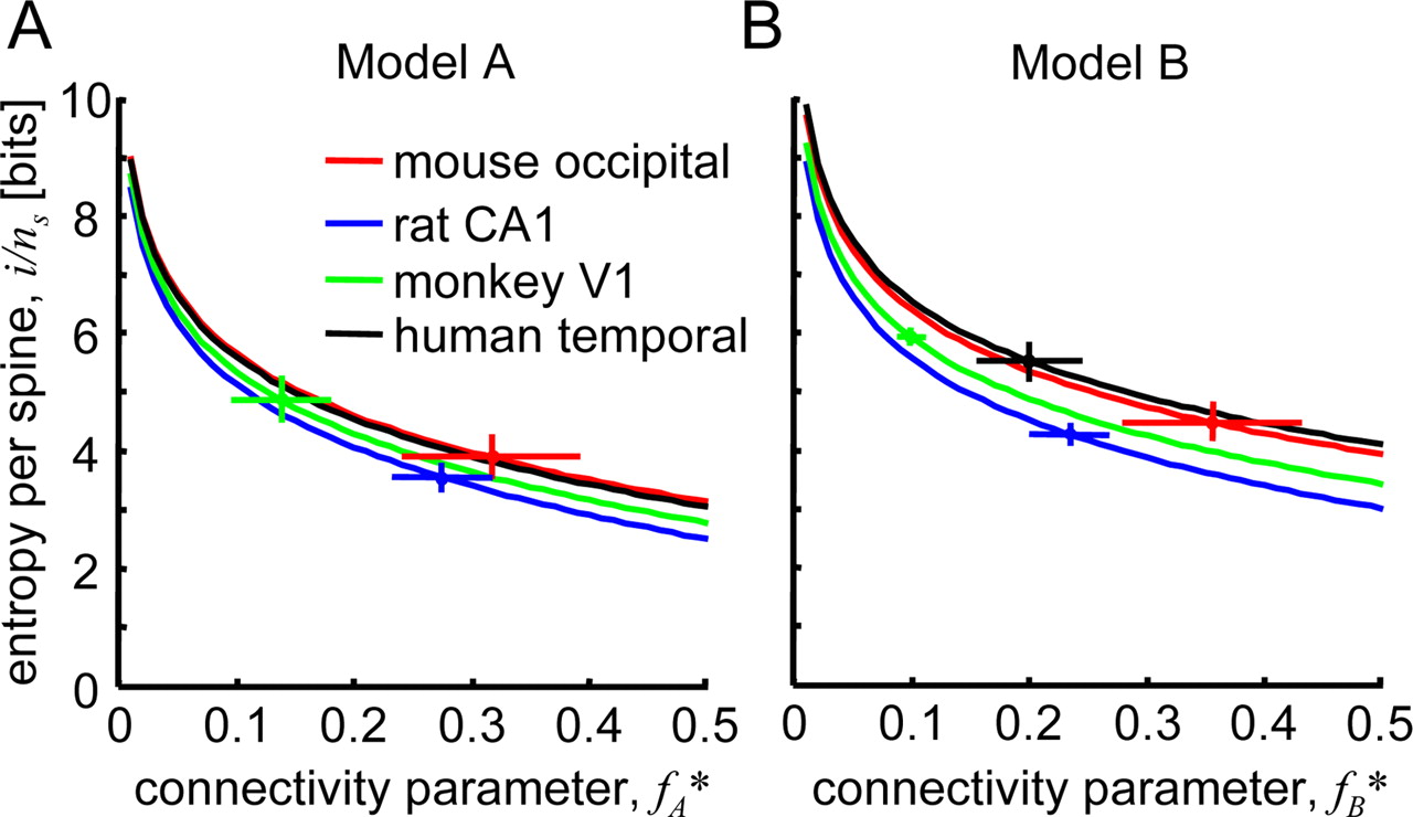
Structural entropy per spine as a function of connectivity parameter f*. A, B, Results based on models A and B for mouse occipital cortex (red), rat CA1 (blue), monkey V1 (green), and human temporal cortex (black). The dots in these figures indicate the connectivity parameters, f*, and the corresponding values of structural entropy per spine, i/ns, calculated based on data from Tables 1 and 2. Error bars indicate SEM.
Selectivity of postsynaptic neurons in their choice of presynaptic partners
We considered a model of synaptogenesis by structural spine remodeling where creation of new synapses between axonal and dendritic branches requires the following three steps. First, the presynaptic axon has to be within the spine reach of the postsynaptic dendrite, i.e., the two branches must be in potential contact with each other. Second, a dendritic spine or filopodium has to find and establish an initial contact with the axon. Finally, based on the functional properties of the neurons this connection could be stabilized and transformed into a synapse or be eliminated.
Consider a potentially connected pair of axonal and dendritic branches. This potential connection may or may not contain an actual synaptic contact. The probability that potentially connected branches are synaptically coupled is given by the connectivity fraction f (s). According to the above model of synaptogenesis, this probability is equal to the product of the probability for a dendritic spine of length s to find the axon, p (find|s), and the probability for this initial contact to stabilize and transform into an actual synaptic connection, p (stabilize|found). Hence,
 Probabilities f (s) and p (find|s) depend on the distance s between the branches. The conditional probability p (stabilize|found), however, is independent of the geometrical details of circuit organization. This probability is only dependent on functional properties of the neurons. It reflects the selectivity of cortical neurons in their choice of synaptic partners.
The fact that the probability p (find|s) has to be less or equal to one for all values of the parameter s allows us to obtain the lower bound for the probability p (stabilize|found) in the following way:
 In the last expression, fmax is the maximum value of the connectivity fraction f (s) (Fig. 3B1–B4).
We estimated the lower bound of p (stabilize|found) based on the values of fmax from Table 2. Our results show that rodent postsynaptic excitatory neurons are not very selective in their choice of presynaptic targets. These neurons make synaptic contacts with >21–30% of presynaptic axons encountered with new spine growth. Primate neurons appear to be more selective making synaptic connections with >7–15% of encountered axons.
Discussion
In this study, we described a theoretical framework for the analysis of the potential of neuropil to undergo structural synaptic remodeling. We considered two models of synapse formation by structural spine remodeling. In the first model, dendritic spines could establish new synapses in the neuropil wherever the presynaptic axonal branch is located sufficiently close to the postsynaptic dendritic segment. In the second model, the presence of a bouton on the presynaptic axonal branch was required for the formation of new synapses. We introduced two measures of the potential of neuropil for structural synaptic reorganization: the connectivity fraction and the structural synaptic entropy. These structural parameters of neural circuit plasticity depend on the shape of dendritic spine length distribution function and other neuropil characteristics that are routinely measured with light or electron microscopy. The connectivity fraction and structural synaptic entropy can be used to assess the learning and memory capacity of neural tissue in its normal or diseased state and make interareal or interspecies comparisons.
Based on the published anatomical data, we evaluated the connectivity fraction in mouse occipital cortex, rat CA1, monkey V1, and human temporal cortex. The connectivity fraction was defined as the ratio of the numbers of actual to potential synapses in the given small range of spine lengths. As a result, the connectivity fraction is equivalent to the probability of finding an actual synaptic connection at a potential synaptic site. We found that the average connectivity fraction in rodent cortex (0.14–0.24) is significantly higher than that in primate cortex (0.051–0.10). Hence, on average, a dendritic spine can choose among 4–7 potential targets in rodents and 10–20 potential targets in primates. Because our comparisons involved different species and cortical areas, it is not clear whether these differences arise from differences between species or cortical areas, or are the result of the combination. New experiments are needed to resolve these questions. Previously (Stepanyants et al., 2002), we reported the values of the connectivity parameter fA* for mouse neocortex, rat CA1 (based on CA3 to CA1 projection), and monkey V1. Despite some differences in methodology and anatomical datasets used, our previous results are not significantly different from the results of this study.
We calculated the entropy associated with building different synaptic circuits out of the scaffold of overlapping axonal and dendritic branches in the neuropil. This entropy reflects the number of structurally different circuits that can be achieved by spine remodeling. It is expected that this number of structurally different circuits exceeds the number of circuits that have different functional properties. This is because some structural connectivity patterns that differ in the placement of individual synapses will result in the same functional circuit on the level of individual neurons or neural networks. As a result, the structural synaptic entropy provides only the upper bound to the amount of useful (functional) entropy in the neural network that can be accessed with spine remodeling. Yet, structural synaptic entropy is expected to be correlated with the amount of useful entropy and, as such, could be viewed as a measure of circuit plasticity and memory storage capacity. We found that the potential of neuropil for structural circuit remodeling is highest in rat CA1 (7.1–8.6 bits/μm3) and lowest in monkey V1 (1.3–1.5 bits/μm3). We do not know which of the considered models of synaptogenesis (A or B) is more appropriate. It is likely that both mechanisms of new synapse formation are used in the brain. In this case, our results only describe the limiting scenarios. Yet, the average difference in structural synaptic entropy for the two models is only ∼15%, suggesting that our estimates are informative regardless of the model details.
One of the approximations made in this study is that the density of asymmetric synapses is close to the density of excitatory boutons (justified above in Materials and Methods, Assumptions and approximations). Although the expressions for the connectivity fractions (Eq. 8) were derived for an arbitrary asymmetric synapse to bouton ratio, in all of the numerical results, this fraction was set to 1. In general, asymmetric synapse to bouton ratio is greater than 1 and it would proportionally increase the connectivity parameter (Eq. 8) and decrease the structural synaptic entropy per spine. However, the latter decrease is expected to be small because of the slow dependence of the structural synaptic entropy on the connectivity parameter in the 0.1–0.4 range (Fig. 5).
Another approximation made in our model was in treating dendritic spines as straight segments that extend perpendicularly from postsynaptic dendritic branches connecting them to presynaptic targets. Although by and large dendritic spines in light microscopy images appear to be quite straight and extend predominantly perpendicularly to dendritic shafts, our results underestimate the amount of structural synaptic entropy. This is because we did not account for the excess entropy associated with spine conformations which could result in new connectivity patterns. The number of potential synapses accessible to spines in the [s − Δs/2, s + Δs/2] length range is proportional to ΔAA = 2baΔs in model A, the cross-sectional area per spine of a cylindrical shell surrounding an axon where the presynaptic dendritic branches are located (see Materials and Methods). In model B, this number is proportional to ΔAB = 2π (s + δ) Δs, which is the cross-sectional area of a spherical shell surrounding a bouton. With new spine conformations these cross-sectional areas increase to ÃA,B, leading to a proportional increase in the number of potential synapses and a decrease in the connectivity fraction, f̃A,B(s) = fA,B(s)ΔAA,B/ÃA,B. To estimate the increase in structural entropy per spine resulting from this effect, we note that, in the limit of small connectivity fractions, the second term in Equation 15 can be neglected and
 Hence, because of different spine conformations, structural entropy per spine increases in the amount equal to the average logarithm of ÃA,B/ΔAA,B and can be large in absolute terms. However, the role of this term in comparing structural entropy per spine between different systems is much smaller. To illustrate this point consider comparison between two systems, with spine length distribution functions p1(s) and p2(s), in model A. Difference in the conformational entropy terms in these systems is as follows:
 Because of the fact that the spine length distribution functions are normalized to unity this expression reduces to the following:
 It is not clear how ÃA depends on s, but because of the slow nature of the logarithm function, the resulting integral is small (fraction of 1 bit for the considered systems) for all reasonable dependencies. Moreover, because ÃA is expected to increase with s, accounting for conformational entropy of dendritic spines only enhances the difference in structural entropy per spine between rodent and primate groups.
Excitatory neurons in regions of the cerebral cortex differ in their functional properties. In the primary visual cortex; for example, neurons differ in their ocular dominance and orientation preference (Hubel and Wiesel, 1963). These neurons connect to each other based on the similarity of their functional properties (Hebb, 1949; Kisvárday et al., 1997; Stettler et al., 2002). It is not entirely clear how many different neuron types are there in the visual cortex. In other words, what is the probability that two nearby randomly chosen excitatory neurons would establish a synaptic contact given the opportunity? One may think that this probability is quite small, <10% based on the dual intracellular recordings from nearby neuron pairs (Thomson and Morris, 2002). This view is also supported by the traditional Hubel and Wiesel (1977) model of the hypercolumn, which contains neurons with different ocular dominance and orientation properties. The question of selectivity of excitatory neurons becomes even more obscure in the nonprimary cortical areas where functional classification of neurons is often unknown. We estimated the lower bound of selectivity of neurons in their choice of synaptic partners based on the shape of the spine length distribution function and average anatomical parameters of neuropil microarchitecture. We showed that postsynaptic excitatory neurons in rodents make synaptic contacts with >21–30% of presynaptic targets (axons in model A, boutons in model B) encountered with new spine growth. Primate neurons appear to be more selective making synaptic connections with >7–15% of encountered targets. This estimate allows us to define the number of functionally different neuron classes in a given region of the cerebral cortex as the inverse of neuron selectivity. According to this measure, in the considered areas of rodent cortex, there are at most three to five functionally different classes of neurons. In the primate cortical areas, the number of functionally different classes of neurons could be much higher. It is only limited from above by our estimate of 7–14 neuron classes.
The values of parameters of structural plasticity calculated in this study are only as good as the anatomical data that were used for the calculations. There is substantial variability in some anatomical measurements performed in different laboratories. One part of this variability is biological in nature. Parameters of cortical neuropil can be highly variable among individual animals (same species, age, and brain area). This interbrain variability is reflected in the error bars reported in this study. We made conservative estimates of SEs to the mean values of all of the calculated parameters. As described in Materials and Methods, true SEs are expected to be much smaller. Another part of variability in anatomical measurements, not captured by our error bars, is caused by different biases introduced by different experimental procedures. To minimize the effect of experimental biases, when possible, we used results that are corrected for experimental artifacts (tissue shrinkage or hidden spines), are based on large numbers of animals, and results that are agreed on by several experimental laboratories. One example that has to be mentioned is the volume density of asymmetric synapses in layer 3 of mouse occipital cortex. As reported in the studies by Schüz and Palm (1989) and Braitenberg and Schüz (1998), this density is 0.91 μm−3 (n = 3 mice). However, the density of asymmetric synapses averaged across all cortical layers of mouse visual cortex was estimated at 2.2 μm−3 (n = 1 mouse) in the study by DeFelipe et al. (2002). We chose not to use the latter density because it is based on measurements from a single animal, and it is averaged across all cortical layers; thus, the exact value for layer 3 is not known. It is also likely that the discrepancy in this case could have resulted from methodological differences. The results for the mouse occipital cortex would change significantly had the 2.2 μm−3 density of asymmetric synapses been used. In this case, the connectivity parameters would decrease to fA* = 0.13 ± (0.03), fB* = 0.14 ± (0.02), and the average connectivity fractions to f̄A = 0.075 ± (0.015), f̄B = 0.056 ± (0.009). The average entropy per spine would increase to 5.3 ± (0.3) bits in model A and to 5.9 ± (0.2) bits in model B, and the average entropy per volume to 11.7 ± (1.6) and 12.9 ± (1.7) bits/μm3, respectively.
By analyzing anatomical parameters measured in different brains, we ignored possible correlations among these parameters. These correlations could significantly affect the results of our calculation. For example, animals with low densities of asymmetric synapses could have higher dendritic or axonal length densities. As a result, the connectivity fraction in these animals would be lower than predicted. To resolve this issue, all of the parameters present in Table 1 must be measured in the same tissue. Such efforts are already under way. One promising approach here is an automated three-dimensional reconstruction of neuropil volume imaged with electron microscopy (Briggman and Denk, 2006; Jain et al., 2007; Mishchenko et al., 2008). This method has the potential to measure reliably spine length distribution, interbouton and interspine intervals, and the density of asymmetric synapses, all in the same small neuropil volume. It will undoubtedly lead to more precise estimates of the connectivity fraction and structural synaptic entropy.
Footnotes
-
This work was supported by the National Institutes of Health Grant NS047138. We thank Zlatko Vasilkoski from Northeastern University, and Quan Wen, Yuriy Mishchenko, and Dmitri Chklovskii from the Howard Hughes Medical Institute, Janelia Farm, for numerous discussions related to the subject of this study as well as for insightful comments on this manuscript.
- Correspondence should be addressed to Armen Stepanyants, Department of Physics, Northeastern University, 110 Forsyth Street, Boston, MA 02115. a.stepanyants{at}neu.edu


