

Abstract
The advance of Parkinson's disease is associated with the existence of abnormal oscillations within the basal ganglia with frequencies in the beta band (13–30 Hz). While the origin of these oscillations remains unknown, there is some evidence suggesting that oscillations observed in the basal ganglia arise due to interactions of two nuclei: the subthalamic nucleus (STN) and the globus pallidus pars externa (GPe). To investigate this hypothesis, we develop a computational model of the STN–GPe network based upon anatomical and electrophysiological studies. Significantly, our study shows that for certain parameter regimes, the model intrinsically oscillates in the beta range. Through an analytical study of the model, we identify a simple set of necessary conditions on model parameters that guarantees the existence of beta oscillations. These conditions for generation of oscillations are described by a set of simple inequalities and can be summarized as follows: (1) The excitatory connections from STN to GPe and the inhibitory connections from GPe to STN need to be sufficiently strong. (2) The time required by neurons to react to their inputs needs to be short relative to synaptic transmission delays. (3) The excitatory input from the cortex to STN needs to be high relative to the inhibition from striatum to GPe. We confirmed the validity of these conditions via numerical simulation. These conditions describe changes in parameters that are consistent with those expected as a result of the development of Parkinson's disease, and predict manipulations that could inhibit the pathological oscillations.
Introduction
Parkinson's disease is attributed to the death of dopaminergic neurons of the substantia nigra pars compacta (Jankovic, 2008), a brainstem nucleus projecting to virtually all of the basal ganglia. The symptoms of Parkinson's disease include bradykinesia, which is a hallmark of basal ganglia disorders, and is characterized by a general slowing of movement execution (Berardelli et al., 2001). The advance of bradykinesia is highly correlated with the presence of abnormal coherent oscillations within basal nuclei in the beta band frequency (13–30 Hz) (Boraud et al., 2005).
Some evidence suggests that the oscillations observed in the dopamine-depleted basal ganglia may originate from the network composed of two basal nuclei: the subthalamic nucleus (STN) and the globus pallidus pars externa (GPe) (Plenz and Kital, 1999). The STN is a glutamatergic nucleus projecting substantially to GPe (Sato et al., 2000b), while the GPe is a GABAergic nucleus projecting profusely back to STN (Sato et al., 2000a). The STN provides widespread inhibition of all movements (Mink, 1996). Recent computational models suggest that this inhibition permits more accurate choices during difficult decisions (Frank, 2006; Frank et al., 2007), and the optimal level of this inhibition is computed by the STN–GPe circuit (Bogacz and Gurney, 2007). In the diseased state, prominent coherent oscillations in firing rate are observed in both nuclei (Bevan et al., 2002; Boraud et al., 2005; Mallet et al., 2008a,b), as in other basal ganglia structures. It is commonly thought that some of these oscillations could be generated in the STN–GPe network, because the architecture of the circuit (STN exciting GPe and GPe inhibiting STN) is prone to generate oscillatory behavior (Bevan et al., 2002). Experimentally it has been already shown that this circuit can sustain oscillatory delta band activity on its own in in vitro studies (Plenz and Kital, 1999). However, the existing experimental data does not provide a clear answer as to whether beta band activity can be produced in the STN–GPe circuit (Lang and Zadikoff, 2005).
To shed light on the origin of oscillations associated with Parkinson's disease, many computational models have been proposed (Gillies et al., 2002; Terman et al., 2002; Frank, 2006; Humphries et al., 2006; Leblois et al., 2006; Gillies and Willshaw, 2007; van Albada and Robinson, 2009). These models provide interesting conclusions and explain experimentally observed phenomena; however, most have a drawback in that the complexity of the equations used in the model make them unsuitable for mathematical analysis. Furthermore, none of them have been able to produce beta oscillations associated with bradykinesia.
In the present study, we develop a computational model of the STN–GPe network, based upon anatomical and electrophysiological studies. The model is detailed enough to reproduce multiple experimental studies showing the reciprocal connectivity between STN and GPe, while being straightforward enough to permit mathematical analysis of the system. This allows us to identify a simple set of necessary conditions on model parameters that guarantees the existence of beta oscillations. These conditions predict manipulations that could reduce the pathological oscillations.
Materials and Methods
In this section, we provide a detailed description of the model of the STN–GPe circuit. We then describe how parameter values in the model were obtained on the basis of experimental data.
Computational model
The architecture of our model is shown in Figure 1A. The STN–GPe network is a mutually coupled system, where STN neurons project excitatory glutamatergic axons to the GPe (Sato et al., 2000b), while GPe neurons project inhibitory GABAergic axons to the STN and to other neurons within GPe (Sato et al., 2000a). Additionally, these two nuclei receive inputs from cortex and striatum, respectively (Kita, 2007). To characterize the firing rate of neural populations in STN and GPe, we use the well described firing rate model (Dayan and Abbott, 2001; Vogels et al., 2005). The differential equation used by this type of model to describe the changes in the firing rate of a neuronal population has the following form:
 where v is the firing rate of the neural population being modeled, v̇ denotes the rate of change in the firing rate (i.e., derivative of v), u⃗ is a vector of firing rates of the presynaptic neural populations, w⃗ is a vector of weights describing strengths of synaptic connections from the presynaptic populations, τ is the time constant describing how rapidly the population reacts to its inputs, and F( · ) is the input–output relationship of the neurons in the steady state, typically termed the activation function or F–I relationship. Using Equation 1 to model STN and GPe populations, we obtain the following set of differential equations describing our system:
 where STN and GP are, respectively, the firing rates of the STN and GPe neural populations. Ctx and Str are the constant inputs from cortex and striatum, respectively. Although beta oscillations have been reported in the cortex and the striatum (Courtemanche et al., 2003; Sharott et al., 2005), we wish to explore whether the STN–GPe network could generate beta oscillations independently of an external oscillatory drive. Consequently, we do not explicitly model corticostriatal interactions and consider these inputs to be constant, and in this way, we ensure that any oscillatory phenomena appearing in our model will be exclusively due to the STN–GPe network. τS and τG are the time constants for STN and GPe populations, respectively. FS( · ) and FG( · ) are the input–output relationships for STN and GPe populations. wAB are the weights of the connections from neural population A to neural population B. ΔtAB are the transmission delays of connections from population A to population B, respectively. Here the indexes A and B used to indicate different neural populations can be any of the following: S for STN, G for GPe, C for cortex, or X for striatum. For clarity, we refer to this set of equations as the “original model,” to distinguish it from the two simplified models we consider in the Results section.

Schematic diagrams of the three computational models considered in the paper: A, original model; B, delayed linear model; C, nondelayed linear model. Each rectangle denotes a nucleus. The excitatory connections are denoted by arrows, while the inhibitory connections by lines ended with circles. The parameters associated with each connection (weights w and transmission delays Δt) are also shown. The indexes of those parameters refer to the origin and target nuclei of the connection, and these can be any of the following: cortex (C), striatum (X), subthalamic nucleus (S), or globus pallidus pars externa (G).
Determining model parameters from experimental studies
For many of the parameters of the model, we were able to determine their values on the basis of published experimental studies. We used the results of experimental studies from monkeys, unless stated otherwise. Table 1 lists the parameters of the model and experimental studies from which they were estimated; these parameters describe the following properties of the model:
Values of the parameters of the model and sources used to establish each value
Connection delays Δt.
In our model, we consider the existence of a transmission delay between STN and GPe neurons. We were unable to find experimental studies investigating the delay in transmission from GPe to STN in monkeys, and hence used the value from an analogous study in rat (Fujimoto and Kita, 1993). We were also unable to find studies investigating transmission delays between two GPe neurons. However, given that these neurons are located closer to each other than STN neurons to GPe, we assume that the corresponding time delay between GPe neurons is shorter than that between GPe and STN neurons.
Time constants τ.
The time constant of a firing rate model corresponds to the membrane time constant of the neurons being modeled (Dayan and Abbott, 2001). Hence, we chose the values of the time constants on the basis of electrophysiological studies of STN and GPe neurons (Kita et al., 1983; Nakanishi et al., 1987b; Kita and Kitai, 1991; Paz et al., 2005).
Firing rates of cortical Ctx and striatal Str neurons.
As mentioned in the previous subsection, the firing rate of cortex and striatum are assumed constant in the model (as we wished to explore whether the STN–GPe network can generate oscillations without external oscillatory input). The firing rates of cortex and striatum were determined from experimental studies where the mean activity of motor cortex and striatal medium spiny neurons were measured (Schultz and Romo, 1988; Lebedev and Wise, 2000).
The activation function F( · ).
The firing rate of STN and GPe neurons as a function of injected current has been studied in detail (Nakanishi et al., 1987a; Kita and Kitai, 1991; Hallworth et al., 2003; Wilson et al., 2004; Deister et al., 2009). All STN neurons reported in these studies showed very similar activation functions with a characteristic sigmoidal shape (Hallworth et al., 2003; Wilson et al., 2004), and hence the activation function for the population of STN neurons in our model is sigmoidal. There exist some studies of GPe neurons whose activation functions were close to sigmoidal (Deister et al., 2009), while other studies reported that different GPe neurons had different activation functions (Nambu and Llinas, 1994). Nevertheless theoretical studies have shown that a population of neurons with heterogeneous activation functions can be approximated in a population level model by a unit with a sigmoidal activation function (Wilson and Cowan, 1972). Therefore, the population of GPe neurons in our model also has a sigmoidal activation function. The activation functions of STN and GPe in our model are shown by solid lines in Figure 2. A sigmoidal curve can be defined with four parameters—its minimum firing rate, its maximum firing rate, its maximum slope, and the firing rate in the absence of inputs. For both STN and GPe, we define the minimum firing rate as 0, as this is the minimum possible neuronal firing rate and it is the common figure observed in experimentally obtained F–I curves. Also in both STN and GPe, the slope will be defined as 1 (note in Fig. 2 that in a wide range the activation function is parallel to dashed-dotted line with slope 1), as this creates a simple interpretation of the units of synaptic weight in our model (see Results). The remaining two parameters, maximum firing rate and the firing rate in the absence of input, are enough to constrain a sigmoidal F–I curve. These parameters will be called MS and BS for STN, and MG and BG for GPe (see labeling in Fig. 2), and they can be directly established from electrophysiological observations. We set MS and MG to the maximum observed firing rate in electrophysiological experiments for each nuclei (Hallworth et al., 2003; Kita et al., 2005; Kita, 2007), BG to the firing rate in GPe when all inputs are blocked (through the use of GABA antagonist–agonists and glutamate antagonists) (Kita et al., 2004; Kita, 2007), and BS to the spontaneous firing rate of STN neurons in slices taken from rats (since there is no published corresponding primate data) (Hallworth et al., 2003). In summary, the activation functions are as follows:
 where “in” is the input to the neural population being modeled.

F–I curves of STN and GPe in the model. Solid lines show the sigmoidal activation functions FS and FG (see vertical axis labels). Dotted lines indicate the firing rates in the absence of input, and values of parameters MS, BS, MG, and BG label the vertical axes. Dashed-dotted and dashed lines show two different linearizations of the sigmoidal input–output relationships. Dashed-doted lines have slope equal to 1, while the dashed lines indicate the linearizations performed around the mean firing rate of each nucleus in the steady state.
Estimating network weights in the healthy state
The parameters describing weights of synaptic connections cannot be directly established from published experimental data. We now describe how we estimate these network weights by finding the values for which the behavior of the model fits a wide array of experimental data on neural activity in STN and GPe.
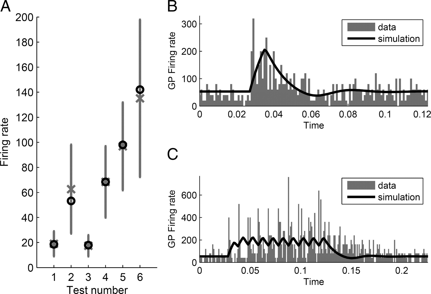
The experimental data recordings of STN and GPe activity used to fit the model can be divided into two types: passive and active. The passive recordings are a group of measures of mean STN and GPe firing rates. These measures have not been exclusively collected in control conditions, but also following injecting glutamate and GABAA blockers into the nuclei, a scenario that we modeled by setting the related connection weights to zero. These passive measures are listed in Table 2 and plotted in Figure 3A. On the other hand, active measures are the recordings of GPe activity performed while electric current is injected into STN. In one such experiment by Kita et al. (2005), two types of STN stimulation were used: single pulse (Fig. 3B) and burst high-frequency stimulation (BHFS), which consists of a train of 10 pulses spanned 0.01 s from each other (100 Hz) (Fig. 3C). The data from this experiment are particularly suitable for the estimation of the synaptic weights in the STN–GPe circuit, because, as concluded by Kita et al. (2005), the responses observed in this study resulted from intrinsic connections of this circuit.
Experimentally observed STN and GPe firing rates in different experimental conditions used to constrain the model

Comparison of model behavior with experimental data obtained from healthy monkeys. Vertical axes indicate firing rate in units of spikes per second. A, Measures of STN′s and GPe's mean firing rate in different experimental situations, as shown in Table 2. Gray crosses show the mean values and vertical lines indicate SDs. This is compared with the mean firing rate of the model in the same situations indicated by black circles. The numbers under the x-axis correspond to the numbers shown in Table 2. B, GPe firing rate after single stimulation of STN (Kita et al., 2005). Gray bars show experimental data and black curve corresponds to the results of simulation. C, GPe firing rate after burst high-frequency stimulation of STN (Kita et al., 2005).
The estimation of network weights was performed using a computational search with an advanced genetic algorithm (Goldberg, 1989; Mitchell, 1998). We term it advanced because it introduces a number of important improvements over a classical genetic algorithm [specifically crossover, elitism, local hill climbing with inertia, stochastic universal sampling, automatic variation of mutation step, fitness sharing, and old elite genes freezing (Goldberg, 1989; Mitchell, 1998)]. An in-depth description of this algorithm falls out of the scope of this paper; however, we provide a brief summary for completeness. For each set of experiments whose results are shown in Figure 3, values of model parameters were estimated using this genetic algorithm, which found the parameter set that minimized the error of the simulation with respect to the experimental recordings, defined as follows:
 where FRexMean,j, GPexSingle, and GPexBHFS are the experimental firing rates of STN or GPe in the three types of experiment (mean firing rates of STN and GPe in six different situations, single stimulation of STN and BHFS stimulation of STN, respectively). FRmean,j, GPsingle, and GPBHFS are the firing rates obtained in the simulations of the model corresponding to each one of the three mentioned types of experiment. The index j refers to the specific experiment where the mean activity of the nuclei was recorded, and it corresponds to the index used in Figure 3A. tsingle and tBHFS are the numbers of bins in the firing rate histograms in Figure 3, B and C. qmean, qsingle, and qBHFS are coefficients that assign more relevance to the experiments that we thought were more important to be reproduced closely. The value of these coefficients are 0.8, 0.1, and 0.1, respectively, which are chosen to optimize the algorithm's performance, based on our experience. The overbar x̄ used in some variables denotes the mean value of that variable in the experimental data, which is used throughout the equation to normalize squared error measures.
The stimulation of STN was simulated by increasing its input by a value proportional to the electrode current used and during the periods of time that the real stimulation lasted. This added quantity corresponds to the term IeStim added to Equation 2:
 In this equation, the term Ie corresponds to the stimulation current in milliamps used in experiments by Kita et al. (2005). Stim is a conversion factor relating electrode current (in milliamps) to the modification induced in neuronal firing rate. This conversion factor is also found by the genetic search together with the network weights. The resulting parameter values are shown in Table 3. A comparison of model behavior with different experimental measures is presented in Figure 3, where the model essentially reproduces a low-pass-filtered version of the firing rate, in accordance with theoretical studies of the firing rate model (Dayan and Abbott, 2001).
Estimated parameter values for synaptic connection weight and electrode stimulation (i.e., Stim)
The range of the weight values obtained is in accordance with known STN–GPe functional interconnectivity. To start with, it is widely accepted that STN axons are diffuse, such that every GPe neuron receives inputs from a large number of STN neurons (Sato et al., 2000b). Similarly, diffuse projections are observed in the axons projecting from striatum to GPe, where each GPe neuron receives inputs from a large number of striatal cells (Kita, 2007). These two similar situations, where on average each GPe cell is influenced by many presynaptic striatal and STN neurons, are in accordance with the high values we obtained for the weights wSG and wXG. Conversely, GPe axons project to small areas of both STN and itself (Sato et al., 2000a). This significantly limits its ability to contact a high number of postsynaptic neurons, and therefore could explain the smaller values obtained for wGG and wGS compared to wSG and wXG. At the same time, although local GPe axons project mainly inside the dendritic tree of the presynaptic neuron (Sato et al., 2000a), they show relatively large boutons contacting the soma and proximal dendrites of postsynaptic cells (Kita, 2007), which would explain the relatively high value of wGG in comparison to wGS.
Simulating the advance of Parkinson's disease in the model
Experimental evidence has established that dopamine influences dendritic excitability through the opposite action of D1-like and D2-like receptors (Surmeier et al., 2007); therefore, the loss in dopamine observed in Parkinson's disease produces an important alteration in how neurons respond to their inputs. In particular, the experimental data summarized in Table 4 suggest that the weights of all synaptic connections included in our model increase with dopamine loss. The main reason for this increase is that all synaptic connections in the model terminate either in STN or in GPe and, in both of these nuclei, D2 receptors are present (Shen and Johnson, 2000; Hoover and Marshall, 2004). These receptors reduce synaptic transmission (Shen and Johnson, 2000; Cooper and Stanford, 2001), and hence in the dopamine-depleted state this reduction is likely to be smaller. We now review additional studies suggesting weight increase specifically for individual connections:
Summary of literature supporting increase in specific synaptic weights with the advance of Parkinson's disease
STN to GPe.
Increase in wSG is suggested by a study showing that dopamine reduces the effect of glutamate on GPe neurons (Johnson and Napier, 1997).
GPe to STN.
For wGS, different studies suggest that the influence from GPe to STN is exaggerated in parkinsonian patients: (1) In rodent models of Parkinson's disease, GABA agonists evoke greater currents in STN neurons than in the healthy state (Shen and Johnson, 2005). (2) Dopamine application in the STN of rats reduces the impact of GABAergic inputs in this nucleus (Cragg et al., 2004).
GPe collaterals.
Increase in wGG is suggested by the observation that ambient GABA is increased in animal models of Parkinson's disease (Robertson et al., 1991; Ochi et al., 2000; Schroeder and Schneider, 2002).
Cortex to STN.
For wCS, studies suggesting an increase include the following: (1) In rodent models, STN neurons are excited to a greater extent by cortex in the parkinsonian state (Magill et al., 2001). (2) Currents evoked by AMPA and NMDA agonists are significantly greater in parkinsonian STN neurons of rodent models (Shen and Johnson, 2005).
Striatum to GPe.
Finally, the increase in wXG is supported by the following observations: (1) Striatal activity is increased in Parkinson's disease (Kish et al., 1999; Tseng et al., 2001; O'Donnell, 2003) (in our model, the striatal activity is not directly modified as we simulate the advance of the disease, so the increased impact of striatum on GPe can be modeled by increasing wXG). (2) It is commonly stated that dopamine inhibits the action of striatal neurons projecting predominantly to GPe through the action of D2 receptors (Obeso et al., 2000; Surmeier et al., 2007), so dopamine depletion should increase the activity of such neurons. (3) An increase in wXG is also supported by the previously mentioned increased levels of GABA in animal models of Parkinson's disease (Robertson et al., 1991; Ochi et al., 2000; Schroeder and Schneider, 2002). (4) Dopaminergic depletion enhances the discharge activity of striatal neurons projecting to GPe and their responsiveness to cortical input (Mallet et al., 2006).
The above studies suggest that the advance of Parkinson's disease should be simulated in our computational model by increasing the synaptic weights of the STN–GPe network. However, these studies do not specify quantitatively by how much each synaptic weight should be increased. To estimate how much these weights increase, we fitted the computational model to experimental data recorded from monkey models of Parkinson's disease (see Table 5) using the same method that was previously used to fit data from healthy animals (see above, Estimating network weights in the healthy state). When using this method to estimate the weights of the diseased state, we treated the frequency of oscillations in the same manner as the mean firing rates are treated in Equation 4. The model successfully reproduced several properties of experimental data listed in Table 5, and these are illustrated in Figure 4. The estimated values of synaptic weights in the diseased state are listed in Table 3.
Experimentally observed STN and GPe firing rates and oscillation frequency in monkey models of Parkinson's disease

Comparison of model behavior with experimental data obtained from monkey models of Parkinson's disease. A, Comparison of the experimental measurements shown in Table 5 with the corresponding values observed in the computational model. The numbers under the x-axis correspond to the numbers shown in Table 5. For measurements 7–12, vertical axis indicates firing rate in spikes per second, while for measurement 13 it indicates oscillation frequency in Hz. Black circles correspond to the equivalent values using model simulations, while gray crosses show the mean experimental values. In measurements 8 and 11, gray vertical lines indicate SD, while in measurement 13, the gray vertical line indicates the frequency range observed in studies by Bergman et al. (1994) and Raz et al. (2000). B, Firing rate of the STN and GPe generated by the model for the same parameter values as in A. C, A single cycle of oscillation from B. The horizontal axis shows the phase of the oscillation, where phase 0° corresponds to the lowest GPe firing rate. The vertical dashed line shows the mean value of phase of each nuclei, which was calculated using the standard equation for the mean of a circular quantity (in this case, the phase).
To simulate the advance of Parkinson's disease, we set the weights in simulations corresponding to different stages of disease progression as follows:
 where wAB is the synaptic weight from nucleus A to nucleus B, wABh the weight value corresponding to the healthy state (see Table 3), wABd the value corresponding to the diseased state (see Table 3), and K a parameter that is increased from 0 (corresponding to a healthy state) to 1 (corresponding to the diseased state) to simulate the continuous advance of the illness. Similar changes in STN–GPe synaptic weights to model dopamine depletion have been used in a previous computational model (Humphries et al., 2006).
Results
We have simulated a model describing changes in firing rates of STN and GPe neurons. Connectivity in the model is shown in Figure 1A, and its parameters were estimated from published experimental data. The STN–GPe circuit in our model receives a constant (rather than oscillatory) input from the cortex and the striatum, as we wanted to investigate whether the STN–GPe circuit can generate oscillations on its own. The constant inputs ensure that any oscillations observed in our simulations are generated within the model of STN–GPe network rather than resulting from external oscillatory input. We simulated the advance of Parkinson's disease by increasing weights of synaptic connections terminating in STN or GPe in agreement with existing literature (see Materials and Methods).
Model of the STN–GPe circuit can generate beta oscillations
When the model was simulated with parameter values corresponding to a healthy state, the firing rate of STN and GPe populations converged to a stable state and the model did not produce oscillations (Fig. 5A). The initial changes in the firing rate within the first ∼50 ms in Figure 5A were due to the difference between the initial values of the firing rates of STN and GPe populations at time 0 and the firing rates at the equilibrium, so they reflect the network converging to an equilibrium.

Simulations of the original model. A–C, Firing rate as a function of time for different values of K. D–F, Phase portraits of the system showing the same firing rates as in A–C. G, Range of firing rates of STN as a function of parameter K. A stable steady state is shown with a solid gray line. The unstable steady state is shown with a dashed gray line. The maximum and minimum values in a cycle of oscillations are shown in black. H, Frequency of the oscillations for different values of K. Note that the model predicts a decrease in frequency of oscillation as the weights increase.
Figure 5B shows a simulation of the model with slightly increased synaptic weights (corresponding to a relatively mild dopamine depletion). Although the firing rates converge to an equilibrium, the difference between initial firing rates and the equilibrium causes transient oscillations with decreasing amplitude. The model with these values of parameters produces a transient oscillation whenever the values of the external inputs change.
Figure 5C shows a simulation of the model with synaptic weights increased to the values estimated from monkey models of Parkinson's disease (see Materials and Methods). The model in this state produces sustained oscillations even though the external inputs remain constant. This is a significant finding as it suggests that the connectivity structure of the basal ganglia makes it prone to oscillate, even in the absence of oscillatory inputs.
To better understand the origin of these oscillations (in the next subsection), it is helpful to visualize them in a different manner. Figure 5D–F shows the same simulated neural activity as Figure 5A–C, but now the two axes correspond to the firing rates of the STN and GPe populations, and different points on the black curves correspond to the firing rates in different moments of time. For example, the initial firing rates in Figure 5C for both STN and GPe are equal to 0 Hz; thus, the initial firing rates are represented in Figure 5F as a point with coordinates STN = GPe = 0 Hz (indicated by a gray circle). In Figure 5C, initially both firing rates of STN and GPe increase, which corresponds in Figure 5F to the curve continuing rightward and upward from the initial state. Figure 5C shows that after ∼20 ms from the start of the simulation, the firing rate of STN starts to decrease while the firing rate of GPe still increases. This corresponds in Figure 5F to the curve continuing leftward and upward, etc. Finally, note that the oscillation in Figure 5C corresponds to a closed loop in Figure 5F.
Figure 5G shows the range of firing rates of STN population after the initial transient response as a function of factor K determining how much the weights are increased in the model. Figure 5G demonstrates that up to K ≈ 0.3, the model converges to a stable state, which we will refer to as a stable steady state. But at K ≈ 0.3, a transition occurs (for details, see supplemental material B, available at www.jneurosci.org), after which sustained oscillations occur. For these values of K, there exists a pair of values of STN and GPe firing rates such that if the STN and GPe firing rates are equal to these values, they do not change, but any small perturbation will make the system oscillate. This value of STN firing rate is shown by the dashed line in Figure 5G, and we will refer to it as an unstable steady state. Finally, Figure 5H shows that the frequency of the sustained oscillations is in the range 16–28 Hz; thus, it falls into the beta band, commonly observed in Parkinson's disease (Boraud et al., 2005). Interestingly, the model demonstrates that the frequency of oscillations decreases, as the synaptic weights associated with the onset of Parkinson's are increased. This suggests that as the condition progresses, we should expect a slowing of beta band activity.
Conditions for the onset of oscillations
This subsection describes a simple set of conditions that the model parameters must satisfy for the model to produce sustained oscillations. These conditions are derived analytically, and therefore they specify whether the oscillations are present for any value of parameters. This complements the results of the previous section, which showed that beta oscillations can be generated by the simulated STN–GPe circuit with a specific range of values of parameters that were estimated from the experimental data. Hence the analytic results of this section predict when the STN–GPe circuit produces oscillations even if the model has different parameters from those used in the previous subsection. This property is valuable because it makes our results robust to errors in parameter estimations, and consequently the results can be generalized to other mammalian species.
We now summarize the main findings before going into more technical details. We show below that three conditions need to be satisfied for the model to produce oscillations. First, the excitatory connection from STN to GPe and the inhibitory connection from GPe to STN need to be relatively strong. Biological systems that include both excitatory and inhibitory feedback often produce robust oscillations (Tsai et al., 2008). The reason why the strong excitatory and inhibitory feedback produce oscillations in the model can be understood by considering Figure 5C: ∼10 ms from the start of the simulation, the activity in GPe becomes so large that it starts to inhibit STN, and the STN activity decreases. But the decrease in STN activity reduces excitatory input to GPe, so from ∼20 ms, the GPe firing starts to decrease. The decreased firing rate of GPe reduces inhibition in STN, so from ∼50 ms, the STN firing rate starts to increase, and the oscillatory cycle continues.
Second, the synaptic transmission delays need to be large relative to the time constant describing how rapidly neurons change their firing rate in response to changes in their inputs. Intuitively, the transmission delays need to be sufficiently long to allow STN neurons to “charge” and increase their firing rate while GPe firing rate remains low. If the transmission delays were very short, the increase in STN firing rate would very quickly result in increase in GPe, which would stop any further increase in STN firing rate, and the system would quickly converge to an equilibrium.
Finally, the cortical input to the STN needs to be relatively larger than the striatal inhibition to GPe. Although we assume that the external inputs to the STN–GPe circuit are constant, these inputs need to provide “energy” so the system can generate oscillations. It is common that systems generating oscillations require a constant input: A familiar example would be a whistle or any wind instrument that requires a constant stream of air to generate oscillations in air pressure.
The change in values of synaptic transmission delays and external inputs is relatively smaller in Parkinson's disease than the change in synaptic weights between STN and GPe. Therefore, the increase in these synaptic weights is most likely a critical factor causing the oscillations.
We now turn to the analysis of the model. The original model is difficult to analyze mathematically because of nonlinear activation functions and transmission delays. To investigate the origin of oscillations analytically, we consider two successive reductions of the original model illustrated in Figure 1, B and C. The first reduction consists of approximation of the sigmoidal activation function in the original model by a linear function. We consider two such approximations shown by dashed-dotted and dashed lines in Figure 2. For simplicity of argument, in this subsection we will consider the linearization shown by the dashed-dotted line in Figure 2, and we will come back to the more precise approximation shown by dashed line in the next subsection. The second simplification of the original model is the assumption that both time constants and all transmission delays are equal. Modifying Equation 2 using these simplifications, we obtain the following system:
 and since firing rates cannot be negative, we additionally extend this equation by imposing two lower boundaries along each axis, STN = 0 and GP = 0. Equation 7 will be referred to as “delayed linear model,” to distinguish it from the “original model” (Eq. 2).
To obtain the second reduction (which is suitable for mathematical analysis), we further approximate this delayed dynamical system by linearizing also about the delay using the Taylor expansions of the terms GP(t − Δt) and STN(t − Δt). This approximation for Equation 7 is given by the following (for full details, see supplemental material C, available at www.jneurosci.org):
 where all the terms depend now on t. This system will be referred to as “nondelayed linear model,” to distinguish it from the previous two ones.
For oscillations to occur, a trajectory in the (GP, STN) plane must create a closed loop such as that shown in Figure 5F. Such a closed loop trajectory will exist in the nondelayed linear model (Eq. 8), when the following three conditions are satisfied.
First, the steady state of the STN–GPe system is unstable. Otherwise, the system would converge to a stable steady state and remain there (as in Fig. 5A,B).
Second, the trajectories starting from the neighborhood of the steady state form spirals. An example of such trajectory is shown in Figure 6A. If this condition was not satisfied, the trajectories originating from the neighborhood of the steady state would move away from the steady state and form straight lines or exponential curves. Supplemental material E (available at www.jneurosci.org) shows that the first and second conditions are satisfied when
 and
and
 respectively. Intuitively, both inequalities describe the situation in which the reciprocal synaptic influence between STN and GPe is higher than a value depending on the self-inhibition of GPe neurons. Furthermore, in supplemental material E (available at www.jneurosci.org), we show that the direction of the flow in the spiral is clockwise in the (GP, STN) plane as shown in Figure 6A.

Schematic illustrations of the boundary flow of the nondelayed linear model. Small open circles denote the location of a steady state. Dotted spirals show a trajectory originating from the vicinity of the steady state. Arrows on the axes show the direction of flow on the boundaries. Labels wCSCtx on the vertical axes show locations of a steady state of the flow on the vertical boundary. Lines labeled SṪN = 0 and GṖ = 0 show nullclines—these are lines in which there is no flow in STN and GP directions, respectively. Importantly the nullclines separate parts of the state space with flow in different directions: Below the SṪN = 0 nullcline, the flow is always upward, while above it is downward; below the GṖ = 0 nullcline, the flow is always leftward, while above it is rightward (as indicated by arrows in 4 parts of the state space separated by the nullclines). A, If wCSCtx is above the intersection of the GṖ = 0 nullcline with the vertical boundary, then no steady state appears in the boundary. This is due to the flow on the boundary above the intersection with the GṖ = 0 nullcline not being invariant (i.e., you move away from the boundary if you begin there). B, If wCSCtx is smaller than the intersection of the nullcline GṖ = 0 with the vertical boundary, then a stable steady state appears in this axis (indicated by a small filled circle).
The third condition required for oscillations is that a closed loop trajectory is formed between the intersection of the boundaries and one of the spiral paths. This condition requires some explanation. If the steady state is unstable and the flow of the system follows a clockwise spiral path, then an appropriate flow on each boundary could force a connection of one spiral path with itself to form a closed trajectory as shown in Figure 6A (the different types of the limit cycle that could be created in this manner can be seen in supplemental Fig. 2, available at www.jneurosci.org as supplemental material). As can be seen, under specific conditions, the flow along the boundary could act to redirect a spiral path along the boundary and ultimately reconnect it at an earlier point on the same trajectory. If this happens, the section of spiral path, together with the flow along the boundaries, would form a limit cycle. In the nondelayed linear model (Eq. 8), it can be shown that for certain parameter values the horizontal boundary (STN = 0) conducts the flow first toward the point (0, 0), and then the vertical boundary (GP = 0) from here toward (0, ∞) until it abandons the GP = 0 boundary (see supplemental material F, available at www.jneurosci.org). Abandoning the GP = 0 boundary, it rejoins a spiral path, which closes again afterward when intersecting the STN = 0 boundary.
The condition necessary for the boundaries to behave in this way, is as follows (see supplemental material F, available at www.jneurosci.org):
 A situation in which the condition is not satisfied is shown in Figure 6B where the flow in the boundaries will stop at point (0, wCSCtx) and will not abandon the GP = 0 boundary.
For parameter values found to reproduce the healthy state, the third condition (Eq. 11) strongly holds. This situation is maintained for higher values of K that simulate the advance of the disease. However, the first and second conditions (Eqs. 9, 10), which are false for K = 0, become true when K is increased, giving rise in this manner to the limit cycle.
Comparison of analytical results with numerical simulations
In this subsection, we compare the conditions found analytically for the nondelayed linear model with simulations of the delayed linear and original models to test how well these conditions describe the occurrence of the oscillations in these two progressively more realistic models.
Equations 9–11 describe a surface in parameter space that divides the parameter values for which oscillations occur from values for which they do not. A direct method to test these conditions in the delayed linear and original models is to determine, numerically, regions in parameter space for each model where the oscillations occur, and compare the limits of these regions with the surface defined analytically by Equations 9–11. To find these oscillatory regions in parameter space, a methodical numerical procedure was used: Each of the three parameters critical in Equations 9–11 (wSG, wGS, and Δt/τ) are varied around the values suggested by the literature for the healthy state. For each combination of the three parameters, the system was simulated and the power spectrum of oscillations in STN was calculated. In each simulation, if the oscillations occurred, their frequency was recorded.
The recorded power and frequency of oscillations for each combination of parameters are shown in Figure 7, A and B, where each colored square represents results obtained for a specific combination of parameter values for wSG, wGS, and Δt/τ. These figures show that oscillations arise as parameters wSG and wGS increase, in accordance with Equations 9 and 10.

A–C, Comparison of conditions for the occurrence of oscillations with the simulations of the delayed linear (A) and original (B, C) models for different values of parameters. In each panel, the left column of displays shows the power spectral density of dominant oscillations, and the right column shows their frequency (in hertz). In each display, each of the small squares summarizes the results of simulation with particular values of parameters shown on the axes. For example, the top-left square in the top-left display indicates that for wSG = 2 and wGS = 3 the model did not produce any oscillations, while the top-right square of this display indicates that for wSG = 50 and wGS = 3 the model did produce oscillations, and the display to the right indicates that these oscillations had frequency of 15 Hz. In the simulations of the delayed linear model in A, all parameters were kept as for simulations of the healthy state, except for wSG, wGS, τ, and Δt. The values of wSG and wGS are shown on the axes, τ = 10 ms, i.e., the average of τS and τG in the healthy state, and Δt is equal to 15.3 ms, 12.8 ms, and 10.3 ms in each of the rows, respectively. Analogously, in the simulations of the original model in B, the values of wSG and wGS are shown on the axes, τS and τG are set to the values in the healthy state, and ΔtSG, ΔtGS, and ΔtGG are increased from the values in the healthy state by 10 ms, 7.5 ms, and 5 ms in each of the rows, respectively. In the simulations of the original model in C, all parameters were kept as for simulations of the healthy state, except for τS, τG, ΔtSG, ΔtGS, and ΔtGG, which were set as shown on the axes.
As mentioned in the previous subsection, in the parameter range considered Equations 9 and 10 determine the occurrence of the oscillations. Since they both need to hold for the oscillations to occur, the system should oscillate when the following is true:
 The white curves in Figure 7A show the boundaries defined in Equation 12. They match the regions found in simulations quite well. The dashed curves in Figure 7B show analogous boundaries for the original model where Δt in Equation 12 is taken as the average of transmission delays in the original model (ΔtSG, ΔtGS, and ΔtGG) and τ is taken as the average of τS and τG. In the original model, however, the oscillations' boundaries do not fit the surface defined by Equation 12. The reason for this is that the delayed linear model was obtained by linearizing the original sigmoidal function with a linear function of slope equal to 1 (Fig. 2, dashed-dotted line). This slope is different from the slope of the sigmoidal curve corresponding to a typical state of the network, i.e., the slope at the input commonly received by STN and GPe. For example, in the condition corresponding to a healthy state, the inputs are as follows:

 where the numbers in the above equations correspond to experimentally observed firing rates in the healthy state listed in Tables 1 and 2. The lines parallel to sigmoidal function with these inputs are shown by dashed lines in Figure 2. The slopes of these lines are F′S = 0.201 and F′G = 0.3269. If the original system is linearized around the above inputs, then weights of all connections terminating in STN are multiplied by F′S and the weights of all connections terminating in GPe are multiplied by F′G. Equation 12 then becomes the following:
 Boundaries defined by Equation 15 are shown by solid curves in Figure 7B, and they provide a much closer match to simulations. Nevertheless there is still a discrepancy for high wGS and relatively low wSG where Equation 15 predicts that the oscillations should occur but they are not observed in the simulations. Note, however, that for high inhibitory weight wGS and low excitatory weight wSG the firing rate in the model will be very low, and the slopes of the sigmoidal functions at a typical state of the network for these parameter values would be even lower. Reducing the slopes of the linear approximations moves the boundary toward higher values of wGS and wSG (Fig. 7B, compare the dashed and solid curves), which explains why the model does not produce oscillations for high wGS and low wSG.
Comparison between rows of Figure 7, A and B, reveals that the oscillations become more likely as Δt/τ increases. Although this effect is relatively weak in Figure 7A, it is strong in Figure 7B. This is because in the range of parameters shown in Figure 7A, the second term in the maximum operator in Equation 12 is higher than the first, thus the second condition (Eq. 10) governs the occurrence of oscillations, and Δt/τ does not appear in Equation 10. Therefore, Equation 12 does not predict dependence of occurrence of oscillations on Δt/τ (note that white curves in Fig. 7A do not differ between rows), and indeed the effect of Δt/τ on the occurrence of the oscillations in the simulations is weak. In contrast, for the range of parameters shown in Figure 7B, the first term in the maximum operator in Equation 15 is higher than the second, thus the first condition (Eq. 9) governs the occurrence of oscillations, and Δt/τ does appear in Equation 9. Therefore, Equation 15 does predict the dependence of occurrence of oscillations on Δt/τ (note that white curves in Fig. 7B do differ between rows), and indeed the effect of Δt/τ on the occurrence of the oscillations in the simulations is strong.
Figure 7B also shows that that there exists a separate region in the parameter space with high wSG and low wGS, where oscillations of a higher frequency occur. These oscillations are generated by inhibitory connections within GPe (simulations not shown here demonstrate that when the inhibitory connections within GPe are removed, these oscillations disappear). For the parameter values for which these oscillations occur (high wSG and low wGS), the firing rate in GPe is particularly high. It is known that a system including just inhibitory feedback with delay can generate oscillations (Gore and van Oudenaarden, 2009), but since the power of these oscillations is two orders of magnitude lower than the oscillations generated by the STN–GPe loop (see Fig. 7B), we do not analyze them further.
Figure 7C shows the dependence of power and frequency of oscillations in the original model on synaptic transmission delay and time constant. The boundary defined by Equation 15 matches well the region of the parameter space where the oscillations occur in the simulations. Importantly, Figure 7C shows that the values of Δt and τ influence significantly the frequency of the oscillation, while variations in synaptic weights were not able to produce such significant change (Fig. 7A,B). Intuitively, the reason why Δt and τ influence the frequency of the oscillations is that these two parameters describe how long it takes for information to “traverse the STN–GPe loop,” hence these two parameters determine the period of the oscillations.
A final point of importance is that simulations performed for equivalent parameter values as per Figure 7B, but with striatal and cortical inputs set to zero, do not produce oscillations. This is consistent with Equation 11, which states that cortical excitation is a necessary condition for the existence of oscillations.
Interpretation of the values of synaptic weights
In the previous subsection, we compared Equations 9 and 10 with simulations, but a real test of the validity of these conditions would be a comparison with an neurophysiological experiment. However, before such comparison can be made, one first needs to be able to estimate the values of weight parameters from an experiment. In this subsection, we describe in what units the weight parameters occurring in Equations 9 and 10 are measured, and how they could be estimated from an experiment.
The weights in the model are measured in units that describe the impact of change in firing rate of presynaptic neurons on the firing rate of postsynaptic neurons. To illustrate this, let us consider two neuronal populations A and B, such that B receives excitatory input from population A, and does not receive any other input. Let us initially assume that that population B has a linear input–output transfer function with slope equal to 1 (we made such an assumption for STN and GPe neurons in the delayed linear and nondelayed linear models). Let us denote the firing rate of these populations by A and B, the weight of their connection by wAB, and the membrane time constants of population B by τB. Thus, the dynamics of population B is described by the following: τBḂ = wABA − B. Note that if A is constant, then the firing rate of population B converges to steady state B* = wABA*. This implies that increasing firing rate in all neurons in population A by 1 [Hz] will increase the mean firing rate in population B by wAB [Hz]. This illustrates that wAB is expressed in units that describe the change in firing rate of the postsynaptic population to a unit change in the firing rate of the presynaptic population.
We now argue that the above interpretation of the units of weight in Equations 9 and 10 remains valid if we further assume that B has a nonlinear input–output transfer function F. In this case, the firing rate of population B converges to B = F(wABA). This implies that increasing the firing rate of all neurons in population A by 1 [Hz] will increase the mean firing rate in population B by F′(wABA)wAB [Hz], where F′(wABA) is the slope of the input–output relationship for the present input. However, recall in the previous subsection that the synaptic weights in the original model had to be rescaled by multiplying them by this slope before inserting their values into Equations 9 and 10. Therefore, in summary, the values of synaptic weights wAB in Equations 9 and 10 are expressed in units that describe the increase in the firing rate of population B due to the increase in the firing rate of population A by 1 [Hz], both for linear and nonlinear input–output transfer functions.
The above interpretation is correct when each connection between two populations is considered in isolation (because if B provided feedback to A, the change in B due to change in A will be more complex). Thus for example, the value of wSG could be interpreted as the change in GPe firing to a unit increase in STN firing, if the feedback connections from STN to GPe were blocked.
Discussion
Relationship to other models
There have been a number of other modeling studies that investigated the oscillations present in the basal ganglia (Gillies et al., 2002; Terman et al., 2002; Humphries et al., 2006; Leblois et al., 2006). Two of those studies (Gillies et al., 2002; Terman et al., 2002) also focused on the STN–GPe circuit and found that it can generate oscillatory activity, but the mechanisms that generated these oscillations were very different from our model, as we now describe. Gillies et al. (2002) developed a firing rate model of the STN–GPe circuit that was simple enough to be studied analytically. They found that their model could produce oscillations only if the strength of connections from STN neurons to other STN neurons was increased. Such connections are not present in our model, because we judged that the evidence for such connections (Hammond and Yelnik, 1983; Sato et al., 2000b) was not strong enough to consider that they play a prominent role in information transmission in the basal ganglia. We think that the reason why Gillies et al. (2002) did not find oscillations without these connections is that they did not consider transmission delays between STN and GPe, and our results (Eq. 9) imply that these delays must exist for the oscillations to be present.
Terman et al. (2002) developed a spiking neuron model of the STN–GPe circuit. The main difference with our model is that they did not consider excitatory input to STN from cortex, but instead introduced a rebound mechanism to simulated STN neurons, which was the only means by which the STN neurons could generate activity in their model. Since the rebound mechanism operated on a slow time scale, the oscillations they observed had much lower frequency than the beta range. One possibility why Terman et al. (2002) did not observe beta oscillations is that they did not consider the cortical input to the STN, which, according to our analysis (Eq. 11), is critical for the presence of the beta oscillations.
Two other models simulated a more general circuit including the cortex, the basal ganglia, and the thalamus (Humphries et al., 2006; Leblois et al., 2006). Leblois et al. (2006) observed oscillatory behavior in theta-alpha band for realistic values of transmission delays. Beta oscillations were not observed, but we think this is due to the fact that they did not include the GPe into the architecture of the model (recall that the STN–GPe feedback loop did generate this frequency in our model).
Humphries et al. (2006) observed gamma (30–80 Hz) and slow (∼1 Hz) oscillatory activity. Beta oscillations that we obtain could correspond to their gamma oscillatory activity, as their model includes the STN–GPe network. The higher-frequency activity could be accounted for by the use of a smaller STN–GPe delay. They consider a set of values for conduction delays and synaptic time constants equivalent to a 2 ms transmission delay in our system, which is smaller than the value of 6 ms used in our study. According to our analysis, this smaller delay will make any frequency generated in the STN–GPe subnetwork higher.
Extending the model
In this paper, we considered constant external inputs to the STN–GPe network, as we wished to explore whether this circuit could generate oscillations on its own. In the future, it would be interesting to include the feedback from STN–GPe circuit to cortex and striatum (via the cortico-basal-ganglia-thalamic loop), so that the cortex and striatum provide oscillatory input while simulating Parkinson's disease. It would be very interesting to investigate how gamma oscillations occurring in the cortex propagate in the basal ganglia and interact with the beta oscillations.
Relationship to experimental data
The model replicates two features observed in Parkinson's disease, that were not included among the data to which the model was fitted. The first feature is the striatal hyperactivity of the indirect basal ganglia path, a central property of the classical model of Parkinson's disease (Obeso et al., 2000), which is clearly displayed in our model by the very noticeable increase in striatopallidal synaptic weight (wXGd = 139.4 for the diseased state, wXGh = 15.1 for the healthy state). Second, the model displays the whole range of beta frequencies observed in Parkinson's disease [13–30 Hz (Brown, 2003; Courtemanche et al., 2003; Boraud et al., 2005; Hammond et al., 2007)], and the particular frequency of oscillation depends on the parameter K describing the advance of the disease (see Fig. 5H). Thus the model suggests that different frequencies within the beta band observed in experiments may correspond to different stages of disease progression.
Equations 9 and 10 predict that the reduction in synaptic weights wGS and wSG can stop beta oscillations. Existing data provides support for this prediction. It has been shown that blocking glutamatergic neurotransmission has anti-parkinsonian effects in a variety of rodent and primate models of Parkinson's disease (Greenamyre, 1993; Lange et al., 1997), which provides initial support to this prediction in relation with wSG. Further, it has been shown that the inhibition from GPe to STN is crucial for the appearance of beta oscillations in the STN–GPe network (Baufreton et al., 2005).
Equation 9 also predicts that the beta oscillations can be induced by reducing the time constant τ. Leblois et al. (2006) proposed that the time constant of a neuronal population in their firing rate model is influenced by the relative proportion of fast, i.e., AMPA, and slow, i.e., NMDA, synapses. Thus, the time constant could be reduced by enhancing AMPA transmission and reducing transmission through NMDA receptors. Such an increase in AMPA and decrease in NMDA transmission (corresponding to reduction in τ) has been shown to accompany the onset of Parkinson's disease in rat models (Shen and Johnson, 2005), which gives support to our prediction.
Equation 11 predicts that cortical input is necessary for the presence of beta oscillations. This is consistent with recent results (Gradinaru et al., 2009) that show that the therapeutic effects of the deep brain stimulation in STN can be accounted by direct selective stimulation of afferent cortical axons projecting to this region. Thus, in the framework of our model, the effect of deep brain stimulation could be described by a reduction in wCS.
Experimental predictions
Until now it has not been shown experimentally that an isolated STN–GPe circuit in vitro can produce sustained beta oscillations. It has been discussed that the lack of beta oscillations in vitro may be due to the lack of cortical input in slices (Loucif et al., 2005; Wilson et al., 2006). Our analysis supports this suggestion: Equation 11 states that to generate beta oscillations, STN needs to receive an excitatory input from the cortex. Hence our analysis predicts that to produce beta oscillations in a STN–GPe circuit in vitro, the STN neurons need to be activated (e.g., by application of glutamate or a constant excitatory stimulation).
Our simulations suggest that the beta oscillations observed in Parkinson's disease are produced in the STN–GPe circuit. This predicts that a local application of dopamine to STN and GPe (rather than to the whole brain) should be sufficient to stop beta oscillations and reduce bradykinesia. Furthermore, since we assume that the beta oscillations occur due to increase in weights caused by reduced activation of D2 receptors, the model predicts that an application of D2 agonist (rather than dopamine) should be sufficient to stop beta oscillations.
A further prediction of the model is that we should expect to see a slowing in frequency of beta oscillations as the parkinsonian condition develops. This can be seen from the relationship between frequency of oscillations and increases in synaptic weight parameters (shown in Fig. 5H).
As mentioned in the previous subsection, the predictions of Equations 9 and 10 on therapeutic effect of reduction in wGS and wSG is qualitatively supported by published experiments. However, Equations 9 and 10 also make quantitative predictions on how much wGS and wSG need to be reduced for oscillations to cease. These predictions could be tested by applying different concentrations of the antagonists, measuring wGS and wSG (last subsection of Results), and observing whether the oscillations are present.
Equation 9 also predicts that the beta oscillations can be stopped by increasing the time constant τ. As described in the previous section, this can be achieved by blocking fast AMPA receptors (e.g., with antagonist) and enhancing transmission through slower NMDA receptors (e.g., by reducing the concentration of magnesium ions). The model predicts that such manipulation should stop the beta oscillations. Furthermore, the model predicts that if the time constant is increased gradually, the frequency of the oscillations should initially decrease before the oscillations stop.
In summary, our computational model predicts novel pharmacological manipulations that could inhibit beta oscillations related to bradykinesia. If the predictions of our model are confirmed in animal experiments, we hope that the model can inspire new treatments for Parkinson's disease.
Footnotes
-
A.J.N.H. was fully funded by Caja Madrid Foundation, Madrid, Spain. J.R.T. acknowledges the financial support of the Engineering and Physical Sciences Research Council via Grant EP/E003249/01 “Applied Nonlinear Mathematics: Making it Real.” We acknowledge Kevin Gurney, Peter Magill, and Frank Marten for their pertinent comments on an earlier version of the manuscript.
- Correspondence should be addressed to Rafal Bogacz, Department of Computer Science, University of Bristol, Merchant Venturers, Building Woodland Road, Bristol BS8 1UB, UK. R.Bogacz{at}bristol.ac.uk


