

Abstract
Binocular mechanisms for visual processing are thought to enhance spatial acuity by combining matched input from the two eyes. Studies in the primary visual cortex of carnivores and primates have confirmed that eye-specific neuronal response properties are largely matched. In recent years, the mouse has emerged as a prominent model for binocular visual processing, yet little is known about the spatial frequency tuning of binocular responses in mouse visual cortex. Using calcium imaging in awake mice of both sexes, we show that the spatial frequency preference of cortical responses to the contralateral eye is ∼35% higher than responses to the ipsilateral eye. Furthermore, we find that neurons in binocular visual cortex that respond only to the contralateral eye are tuned to higher spatial frequencies. Binocular neurons that are well matched in spatial frequency preference are also matched in orientation preference. In contrast, we observe that binocularly mismatched cells are more mismatched in orientation tuning. Furthermore, we find that contralateral responses are more direction-selective than ipsilateral responses and are strongly biased to the cardinal directions. The contralateral bias of high spatial frequency tuning was found in both awake and anesthetized recordings. The distinct properties of contralateral cortical responses may reflect the functional segregation of direction-selective, high spatial frequency-preferring neurons in earlier stages of the central visual pathway. Moreover, these results suggest that the development of binocularity and visual acuity may engage distinct circuits in the mouse visual system.
SIGNIFICANCE STATEMENT Seeing through two eyes is thought to improve visual acuity by enhancing sensitivity to fine edges. Using calcium imaging of cellular responses in awake mice, we find surprising asymmetries in the spatial processing of eye-specific visual input in binocular primary visual cortex. The contralateral visual pathway is tuned to higher spatial frequencies than the ipsilateral pathway. At the highest spatial frequencies, the contralateral pathway strongly prefers to respond to visual stimuli along the cardinal (horizontal and vertical) axes. These results suggest that monocular, and not binocular, mechanisms set the limit of spatial acuity in mice. Furthermore, they suggest that the development of visual acuity and binocularity in mice involves different circuits.
- binocularity
- orientation selectivity
- primary visual cortex
- spatial frequency selectivity
- two-photon calcium imaging
- visual acuity
Introduction
The mammalian visual cortex processes spatial information using neurons that are narrowly tuned to specific spatial frequencies (Maffei and Fiorentini, 1973; Schiller et al., 1976a,b; Movshon et al., 1978a,b; De Valois et al., 1982a). Given the narrow bandwidth of cortical responses, neurons tuned to the highest spatial frequencies should set the limit of visual acuity. Psychophysical studies have long suggested that binocular vision enhances spatial acuity over monocular viewing by enhancing the sensitivity of signal detection (Pirenne, 1943; Campbell and Green, 1965; Blake et al., 1981). Together, these observations suggest that individual neurons in visual cortex tuned to the highest spatial frequencies are likely to receive eye-specific inputs whose response properties are well matched. Hubel and Wiesel's initial description of binocular receptive fields reported that eye-specific inputs to cortical neurons are similar (Hubel and Wiesel, 1962). Subsequent studies that explicitly explored spatial frequency tuning in binocular neurons found significant, but quantitatively modest, asymmetries in the preferred spatial frequencies and bandwidth of eye-specific responses (Skottun and Freeman, 1984; Bergeron et al., 1998; Saint-Amour et al., 2004). Other studies, however, found many spatial frequency-mismatched binocular responses in cat visual cortex (Hammond and Pomfrett, 1991; Hammond and Fothergill, 1994).
The mouse system has emerged as a prominent model for studying precise wiring and developmental plasticity in the central visual pathway (Huberman and Niell, 2011; Espinosa and Stryker, 2012). In particular, the spatial acuity of mouse cortical responses has been used extensively to assess cellular and molecular mechanisms for binocular system development (e.g., Huang et al., 1999; Porciatti et al., 1999; Beurdeley et al., 2012; Davis et al., 2015). Because these studies used indirect measures of neuronal activity, such as visually evoked potentials and intrinsic signal imaging, they cannot address whether binocular responses at the level of individual cells are matched at the highest spatial frequencies. Although many aspects of neuronal response properties have been studied extensively in mouse binocular visual cortex (Dräger, 1975; Wagor et al., 1980; Gordon and Stryker, 1996; Mrsic-Flogel et al., 2007; Wang et al., 2010; Scholl et al., 2013), the investigation of spatial frequency tuning in mice has been largely restricted to the monocular zone (Niell and Stryker, 2008; Hoy and Niell, 2015; Durand et al., 2016). Little is known about binocular matching of spatial frequency responses in mouse visual cortex at the level of single neurons.
In this study, we set out to characterize the eye-specific spatial frequency tuning of neurons in the binocular zone of mouse area V1. Using calcium imaging of excitatory neurons, we found that contralateral eye-dominated neurons in binocular area V1 are tuned to higher spatial frequencies than their binocular counterparts. In binocular neurons, responses that are matched in spatial frequency preference are matched in orientation preference, whereas cells mismatched in spatial frequency preference are more mismatched in orientation preference. Furthermore, we found that contralateral eye dominated, high spatial frequency-tuned neurons are biased to the cardinal axes. These results suggest that distinct circuit mechanisms process binocular and high acuity vision in the mouse visual system.
Materials and Methods
Animals.
All protocols and procedures followed the guidelines of the Animal Care and Use Committee at the University of California, Irvine. To image evoked activity in excitatory neurons, a Camk2a-tTA driver line (RRID:IMSR_JAX:007004) was crossed to a line expressing the calcium indicator GCaMP6s under the control of the tetracycline-responsive regulatory element (tetO) (RRID:IMSR_JAX:024742) (Wekselblatt et al., 2016). The founder line was heterozygous for both transgenes and maintained by breeding with wild-type C57BL/6 mice (RRID:IMSR_CRL:642). Wild-type mice were used in experiments for AAV-mediated expression of GCaMP6s. Mice were weaned at P18–P21 and cohoused with one or more littermate until the day of window implantation (P63–P91). In awake recordings, 4 female and 8 male mice were used; whereas in anesthetized recordings, 3 males were used.
Cranial window implantation.
Mice were anesthetized with isoflurane in O2 (2% for induction, 1%–1.5% for maintenance). Headplate attachment and craniotomy were performed in one surgery. Carprofen (5 mg/kg, s.c.) and topical xylocaine (2%, 20 mg/ml) were administered to provide analgesia. Dexamethasone was administered 4–8 h before surgery (4.8 mg/kg, i.m.). Atropine (0.15 mg/kg, s.c.) was administered to reduce secretions and aid in respiration. To attach custom-printed ABS headplates, the skull was cleared of connective tissue and dried with ethanol. A thin layer of Vetbond was applied to the skull and the headplate was attached using dental acrylic at an angle parallel to the site of imaging (∼20 degrees from horizontal). A craniotomy (5 mm diameter) was performed over the left or right hemisphere using previously described methods (Figueroa Velez et al., 2017). A 5 mm glass coverslip (World Precision Instruments) was placed over the exposed brain and sealed with Vetbond and black dental acrylic. Sterile eye ointment (Rugby) was used to protect the eyes. Body temperature was maintained at 37.0°C using a heating pad under feedback control from a rectal thermoprobe. Mice were allowed to recover on a warm heating pad following surgery (<15 min). Mice were given daily injections of carprofen (5 mg/kg, s.c.) for at least 2 d after surgery.
GCaMP6s virus delivery.
To assess visual responses in binocular visual cortex, AAV-Syn-GCaMP6s (Chen et al., 2013) (Upenn Vector Core AV-1-PV2824) was injected into wild-type mice 2 weeks before imaging. Virions were diluted 10-fold with ACSF to ∼2 × 10¹² GC/ml, and 400 nl was injected at a rate of 10 nl/min. Lactated Ringer's (0.2 ml/20 g/h, s.c.) was given to prevent dehydration. Mice were allowed to recover on a warm heating pad following surgery (<15 min).
Widefield visual area mapping.
Mapping of the visual areas was performed at least 1 week after window installation using widefield imaging of GCaMP6s (Wekselblatt et al., 2016; Zhuang et al., 2017). Widefield fluorescence images were acquired using a SciMedia THT macroscope (Leica PlanApo 1.0×; 6.5× 6.5 mm imaging area) equipped with an Andor Zyla sCMOS camera. The surface vasculature and GCaMP6s signal were visualized using a blue 465 nm LED (LEX2). The camera was focused ∼600 μm beneath the surface. Image acquisition and visual stimulus presentation were controlled by custom written software in python using the PsychoPy 1.8 library.
Visual stimuli for area mapping.
To perform visual area segmentation, awake mice were shown a 20° wide visual noise stimulus that swept periodically every 10 s in each of the four cardinal directions. The sweeping visual stimulus was created by multiplying a band-limited (<0.5 c/d; >2 Hz), binarized spatiotemporal noise movie with a one-dimensional spatial mask (20°) that was phase modulated at 0.1 Hz. A gamma-corrected monitor (54 inch LED LG TV model 55LB5900) with maximum luminance of 30 cd/m2 was placed 20 cm from the contralateral eye and angled at ∼30° from the long axis of the animal. The stimulus was spherically corrected to cover 140° visual angle in elevation and 120° in azimuth. The stimulus was presented to the contralateral eye for 5 min for each direction. To confirm the location of the binocular zone, we also presented the sweeping, binarized noise stimulus confined to the central 30° of visual azimuth.
Analysis for area mapping.
Retinotopic maps of azimuth and elevation were used to generate a visual field sign map (Sereno et al., 1994; Garrett et al., 2014) to designate borders between visual areas. Recordings from binocular V1 were confined to regions adjacent to the intersection of the horizontal and vertical meridians at the border of V1 and LM. Recordings from monocular V1 were confined to regions medial to the binocular zone of V1 along the horizontal meridian.
Two-photon calcium imaging.
Fluorescence was gathered with a resonant two-photon microscope (Neurolabware) with 920 nm excitation light (Mai Tai HP, Spectra-Physics). Emissions were filtered using a 510/84 nm BrightLine bandpass filter (Semrock). A 16× (Nikon NA = 0.8) or a 20× water-immersion lens (Olympus NA = 1.0) was used. Image sequences typically covered a field of ∼700 μm × 500 μm and were acquired at 7.7 or 15.4 Hz (1024 lines) using Scanbox acquisition software (Scanbox) at a depth of 200–250 μm below the pia.
Two-photon visual stimuli.
Visual stimuli were generated by custom-written python code using the PsychoPy 1.8 library. Full field sinusoidal gratings of six spatial frequencies (0.03–0.96 c/d, logarithmically spaced) in eight directions (0–315,45° steps) at a fixed temporal frequency (2 Hz) were presented using an Acer V193 gamma-corrected monitor (53 × 33cm, 60 Hz refresh rate, 20 cd/m2). The visual stimulus was spherically corrected. In addition to the 48 grating stimuli, we also showed a blank condition and a condition in which the whole monitor flickered at 2 Hz (FF). The 50 total stimulus conditions were presented in a random order for each of the 10 repetitions. In one subset of experiments, 20 repeats were used. For each trial, the stimulus was presented for 2 s, followed by 3 s of gray screen. For anesthetized recordings, mice were sedated during recordings using isoflurane in O2 (0.6–0.9%) supplemented with chlorprothixene (2 mg/kg, i.p.). For awake and anesthetized recordings, the visual stimulus was presented either first to the ipsilateral or the contralateral eye. In awake recordings, four of eight animals viewed the stimulus through the contralateral eye first. In anesthetized recordings, 2 of 3 mice viewed the stimulus through the contralateral eye first.
Cellular responses.
Custom-written Python routines were used to remove motion artifact, identify cell ROIs, extract calcium fluorescence traces, and perform analyses. First, we implemented motion correction by using an efficient algorithm that corrects for translational artifacts by minimizing the Euclidean distance between frames and a template image using a Fourier transform approach (Dubbs et al., 2016). To identify the region of pixels associated with distinct neuronal cell bodies, we used the maximum intensity projection of the images. Only cell bodies that could be visually identified throughout the 80 min recordings were included in analysis. The fluorescence signal of a cell body at time t was determined as Fcell(t) = Fsoma(t) − (R × Fneuropil(t)) (Kerlin et al., 2010; Chen et al., 2013). R was empirically determined to be 0.7 by comparing the intensity of GCaMP6s signal in the blood vessels to the intensity in the neuropil across recordings. The neuropil signal Fneuropil(t) of each cell was measured by averaging the signal of all pixels outside of the cell and within a 20 μm region from the cell center.
To determine a cell's response to each stimulus trial, the cell's trace during the stimulation period was normalized to the baseline value averaged over the 0.75 s preceding stimulus presentation. The cell's response to a given orientation θi was defined as the average response across the 10 repeats of each condition: F(θi). An estimate of the cell's spontaneous calcium fluctuation was determined using the cell's trace during the blank condition. At each spatial frequency, a cell's responsiveness was determined using a one-way ANOVA (p < 0.01) across orientations against the blank condition (see Fig. 2A). To assess spatial frequency tuning and directional selectivity, we restricted our analysis to neurons whose responses at the peak spatial frequency reached significance and whose responses to drifting gratings across all spatial frequencies reached significance when compared against the blank condition (ANOVA p < 0.01; see Fig. 2B; analyzed cells).
Preferred orientation.
For each cell, preferred orientation (θpref) was determined at the spatial frequency that gave the strongest response by calculating half the mean of the directional vectors weighted by the response F(θ) at each orientation as follows:
 For each spatial frequency, a tuning curve, R(θ), was determined by fitting F(θ) to a sum of two Gaussians centered on θpref and θpref + π, with different amplitudes and equal width, and a constant baseline. The amplitude of the response at the preferred orientation (Rpref) was R(θpref).
Preferred spatial frequency.
To determine the preferred spatial frequency, responses at the preferred orientation (Rpref) across all spatial frequencies were fitted with a difference of Gaussians function (Hawken and Parker, 1987). For each fitted neuron, the preferred spatial frequency was determined by the maximum of the difference of Gaussians functional fit. In addition, the bandwidth was calculated by taking the square root of the width at half the maximum of the fit.
Orientation and direction selectivity.
Orientation selectivity for a cell was determined using a method derived from the circular variance of the cell's response F(θ) (Niell and Stryker, 2008; Kerlin et al., 2010, Hoy and Niell, 2015). The circular variance method for calculating orientation selectivity is closely correlated to an alternative measure that uses a sum of two Gaussians (Figueroa Velez et al., 2017). Because the circular variance-based method is sensitive to the sign of F and because F fluctuates >0 and <0 at baseline (SD ± 0.032% dF/F), we added an offset to F for each cell which set the minimum average response to 0: F(θi)) = F(θi) − min(Fθi). Following this correction, the orientation selectivity index was calculated as follows:
 The direction selectivity index (DSI) was calculated as follows:

Ocular dominance index (ODI).
The ODI for each cell was calculated as (C − I)/(C + I), where C is Rpref for the contralateral eye and I is Rpref for the ipsilateral eye. Contralaterally dominated neurons have an ODI value near 1, and ipsilaterally dominated neurons have an ODI value near −1. In cases where no significant response was detected for one eye, Rpref for that eye was set to 0. Therefore, responses that were purely a result of contralateral or ipsilateral eye stimulation were assigned ODI values of 1 and −1, respectively.
Pupil tracking.
Contralateral and ipsilateral eyes were recorded simultaneously using GigE cameras (Teledyne Dalsa, Mako G). The cameras were positioned 30° above the mouse's eyepoint and 45° from the mouse's midline on each side. The eyes were illuminated by the infrared laser (MaiTai HP, Spectra-Physics) used for two-photon imaging.
To identify the pupils, each frame was thresholded and contours were extracted (Suzuki and Abe, 1985) using routines from the OpenCV library (version 3.2.0). Artifacts that distorted the pupil contours were removed by (1) converting all contours to convex hulls (Sklansky, 1982), (2) filtering the hulls using a predefined range, and (3) assigning the pupil to be the hull whose centroid was located closest to the center of the eye.
Frames in which the contrast dropped significantly or those in which the mouse blinked produced erroneous pupil identification. To address this issue, we established a scoring system that would exclude frames in which the pupil exceeded a maximum circularity score. The circularity score was determined by calculating the ratio between the longest distance from the centroid to the hull and the shortest distance from the centroid to the hull. A score of 1.25 was selected as the cutoff based on the distribution of circular scores for a recording.
Experimental design and statistical analyses.
The statistical determination of cellular responsiveness is described in detail above. The Kolmogorov–Smirnov test was used to assess differences in the distributions of cellular spatial frequency preferences. The Mann–Whitney U test and Kruskal–Wallis test were used to assess differences between groups of cells (e.g., monocular vs binocular cells). For animal-by-animal analyses of median eye-specific differences in binocular responses, we used a pairwise Wilcoxon signed-rank test for comparing two groups and, for more than two groups, a Friedman test with a Dunn's multiple-comparison post hoc test. Correlations were determined using Spearman rank correlation. For the analysis of direction selectivity, a Mann–Whitney U test was used to determine the significance of cardinality for a group and a χ2 test was used to test differences in cardinality between groups. Statistical analyses were performed using Prism v7.01 (GraphPad). To find the SE of the median for preferred spatial frequency of a group of cells, we estimated the sampling distribution using a bootstrap methodology that resampled 500 times with replacement (MATLAB, The MathWorks).
Results
To systematically probe the spatial frequency tuning of binocular area V1, we used a transgenic mouse line that expresses GCaMP6s under the control of the CaMK2 promoter (CaMK2-tTA;tetO-GCaMP6s) (Wekselblatt et al., 2016). The line restricts GCaMP6s expression to excitatory neurons only and excludes inhibitory interneurons, which are known to have distinct spatial frequency tuning properties (Kerlin et al., 2010). Binocular area V1 was identified using a widefield imaging procedure to retinotopically map visual areas in posterior mouse cortex (visual field sign map; Fig. 1A) (Garrett et al., 2014). Next, GCaMP6s imaging of cellular responses was performed using 2-photon microscopy. Recordings were directed to the central visual field by situating the field of view adjacent to the map coordinates for the V1/LM border and centered on the horizontal meridian. Cellular imaging was performed in awake, head-fixed mice that were acclimated to the setup over several days. Mice were shown a visual stimulus through either the contralateral or ipsilateral eye that consisted of 2 s presentations of drifting visual gratings at one of eight directions and one of six spatial frequencies (0.03–0.96 c/d spaced logarithmically; Fig. 1B). We interleaved the presentation of a full field flickering stimulus with the gratings to detect neurons tuned to very low spatial frequencies. Each stimulus condition was repeated 10–20 times per eye. Eye movement and pupil dilation were also recorded for the eye shown the visual stimulus. Half of the fields were imaged with the ipsilateral eye shown the stimulus first and half with the contralateral eye first.

Assessment of binocular spatial frequency tuning in primary visual cortex using GCaMP6s mice. A, Experimental setup. Top left, Widefield imaging produces a visual field sign map that identifies the boundaries of primary visual cortex (V1). Scale bar, 1 mm. Top right, Two-photon imaging was done in central binocular cortex adjacent to the border of areas V1 and LM. Visual responses were measured in head-fixed, awake mice while they viewed drifting sinusoidal gratings. Mice walked freely while pupil dilation and eye movements are tracked by IR camera. B, Each trial consists of a 2 s presentation of a drifting grating at one of eight directions and one of six spatial frequencies, followed by a 3 s off period. The stimulus was shown to either the contralateral or ipsilateral eye. C, Example binocular responses from a cell. Gray boxes represent when the visual gratings were shown. Gray traces represent individual trials. Black represents averaged traces for contralateral eye stimulation. Red represents averaged traces for ipsilateral stimulation. This cell prefers vertical gratings at 0.06 c/d moving along the horizontal axis. D, Four types of spatial frequency responses in binocular V1 revealed by contralateral (black) and ipsilateral (red) eye stimulation: spatial frequency-matched binocular, spatial frequency-mismatched binocular, contralateral monocular, and ipsilateral monocular cells. The average responses at each spatial frequency are overlaid with a difference of Gaussians fit. Preferred spatial frequency is determined by the maximum of the fit. E, F, Maps of spatial frequency preference for contralateral (E) and ipsilateral (F) eye stimulation shown for a field of view. Scale bar, 50 μm. Most neurons are tuned to low spatial frequencies (yellow and green). Higher spatial frequency tuning (cyan and magenta) is found predominantly in contralateral responses.
Typical excitatory neurons responded to low spatial frequencies (<0.12 c/d) and had binocularly matched preferences for spatial frequency and direction (Fig. 1C). The contralateral response (Fig. 1C, black) was typically stronger than the ipsilateral response (Fig. 1C, red). Beyond these binocularly matched, low spatial frequency-preferring responses, three other types of responses are also found in binocular area V1: cells that had mismatched spatial frequency tuning between the two eyes, cells that were dominated by the contralateral eye, and cells dominated by the ipsilateral eye (Fig. 1D). A typical field of view reveals overt differences in the spatial frequency tuning of the contralateral and ipsilateral eye inputs to binocular visual cortex (Fig. 1E,F).
Higher spatial frequency tuning of contralateral eye responses
Together, 1850 cells were imaged in 10 animals. Across all cells, more neurons responded at high spatial frequencies for contralateral than for ipsilateral eye stimulation (Fig. 2A, all cells). To characterize spatial frequency selectivity, we restricted our analysis to those cells (Fig. 2B, analyzed cells) whose responses at the peak spatial frequency reached significance and whose responses to drifting gratings across all spatial frequencies reached significance when compared against the blank condition (p < 0.01, ANOVA, total: 61.6%; contralateral: 48.97%; ipsilateral: 34.59%). These cells also responded to high spatial frequency stimuli through the contralateral and not the ipsilateral eye (Fig. 2B). Composite spatial frequency response curves for all (Fig. 2C) and analyzed (Fig. 2D) cells confirm that these cells responded to high spatial frequencies through the contralateral and not the ipsilateral eye.

Higher spatial frequency tuning of contralateral eye responses in binocular visual cortex. A, Percentage of all recorded cells are plotted with significant responses at each spatial frequency for contralateral eye (black) and ipsilateral eye (red) stimulation. Error bars indicate SE of percentage responsive across 10 animals. B, Spatial frequency tuning and directional selectivity were only analyzed in cells whose responses at the peak spatial frequency reached significance and whose responses to drifting gratings across all spatial frequencies reached significance when compared against the blank condition. Among these analyzed cells, the percentages with significant responses at each spatial frequency are plotted. Error bars indicate SE of percentage responsive across 10 animals. C, D, Composite tuning curves for responses to contralateral (black) and ipsilateral (red) eye stimulation are plotted for all cells (C) and those cells that met our statistical criteria for spatial frequency tuning analysis (D). In both cases, the composite spatial frequency responses to the contralateral eye extended to higher spatial frequencies than the responses to the ipsilateral eye. Error bars indicate SE of response strength across 10 animals.
We found that the preferred spatial frequency of contralateral eye responses in binocular area V1 was overall ∼35% higher than ipsilateral responses (median ipsilateral: 0.073 c/d, contralateral: 0.099 c/d; Fig. 3A,B). The animal-by-animal distributions of preferred spatial frequency for contralateral (black) and ipsilateral (red) responses show a consistent pattern of higher tuning in the contralateral pathway. In contrast, we found that the spatial tuning bandwidths of contralateral and ipsilateral responses were nearly identical (Fig. 3C,D). The amplitude of the response to the preferred stimulus across cells was somewhat higher for contralateral eye recordings (Fig. 3E), raising the possibility that ipsilateral responses at high spatial frequencies were too weak to be detected. We found, however, no relationship between spatial frequency preference and response amplitude in our recordings (Fig. 3F; all responses: r = −0.02; p = 0.556). These results reveal an eye-specific asymmetry in the responses of binocular area V1.
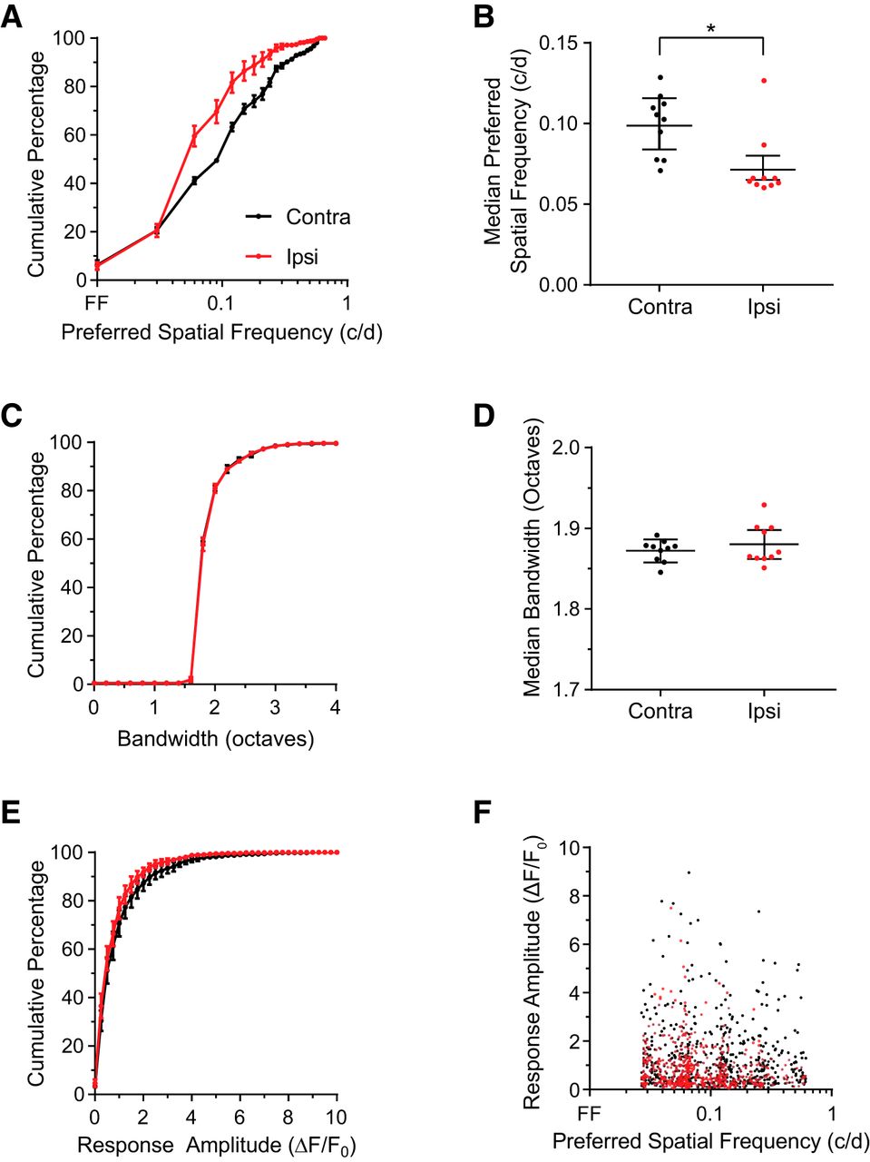
Spatial frequency preferences of contralateral responses are higher than ipsilateral responses in binocular visual cortex. A, Preferred spatial frequency for contralateral (black) and ipsilateral (red) eye responses. The distributions from 10 mice were binned, and the mean is plotted. Error bars indicate SEM. The preferred spatial frequency for contralateral responses is significantly higher than for ipsilateral responses (median contralateral = 0.099 c/d, n = 908 neurons; median ipsilateral = 0.0653 c/d, n = 641 neurons; Kolmogorov–Smirnov test D = 0.178, p < 0.0001; Mann–Whitney U test = 245465, p < 0.0001). B, Data grouped by animal confirm that the preferred spatial frequency of contralateral responses is significantly greater than ipsilateral responses (contralateral median = 0.108 c/d; ipsilateral median = 0.0653 c/d; Wilcoxon's rank sum test = −45, p = 0.0195, N = 10 mice). Error bars indicate SE of the median. C, The spatial frequency bandwidth for contralateral (black) and ipsilateral (red) responses are very similar (contralateral median = 1.867; ipsilateral median = 1.867). Error bars indicate SEM. D, Data grouped by animal confirm that the spatial frequency bandwidths do not differ by eye (contralateral median = 1.876 octaves; ipsilateral median = 1.869 octaves, Wilcoxon rank sum test = 11, not significant, p = 0.6094, N = 10 mice). Error bars indicate SE of the median. E, Averaged responses at the peak spatial frequencies are shown for contralateral (black) and ipsilateral (red) eye stimulation. Responses to the contralateral eye are higher than responses to the ipsilateral eye (median contralateral = 0.620 ΔF/F, median ipsilateral = 0.518 ΔF/F; Kolmogorov–Smirnov test D = 0.084, p = 0.0099; Mann–Whitney U test = 258651, p = 0.0002). F, Peak responses for contralateral (black) and ipsilateral (red) stimulation are plotted against preferred spatial frequency. The amplitudes of contralateral responses are similar at low and high preferred spatial frequencies. *p < 0.05.
Higher spatial frequency tuning of monocular responses
Next, we examined the binocularity of cortical responses in binocular area V1 (Fig. 4A). Surprisingly, we found that 62% of neurons recorded in binocular area V1 responded to one eye only (Fig. 4B; ipsilateral: 19%; contralateral: 43%), whereas the remainder responded to both eyes (gray). The spatial distribution of monocular responses (ODI = 1 or −1; see Fig. 4A) appeared widely dispersed, discounting the possibility that our recordings had been made on the edge of the binocular zone. The number of trials and the order of eye presentation were also not found to be a factor in the prevalence of monocular responses.

Contralaterally dominated cells are tuned to higher spatial frequencies than binocular and ipsilaterally dominated cells. A, ODI was calculated as follows: C − I/C + I. Single cells are color coded by ODI (N = 10 mice, n = 994 cells) for cells in binocular V1 (bV1). Scale bar, 50 μm. B, Gray represents binocular cells. Red represents cells that respond to the ipsilateral eye only. Black represents cells that respond to the contralateral eye only. Error bars indicate SE across animals (overall ODI = 0.268; binocular only ODI = 0.117, n = 994 cells, N = 10 mice). C, Binocular responses to the contralateral eye (gray dots) and ipsilateral eye (transparent green dots) are plotted as a function of ODI. Solid lines indicate binned averages. Monocular responses to the contralateral eye (solid black dots) and ipsilateral eye (solid red dots) are shown with their averages plotted as squares. D, Preferred spatial frequency for contralateral monocular (black), ipsilateral monocular (red), binocular (gray) cells, and cells recorded in mV1 (blue). The preferred spatial frequency of the dominant eye response was used to plot the distribution for binocular cells. In binocular V1, the spatial frequency preferences for contralateral monocular cells are higher than for binocular cells and ipsilateral monocular cells (contralateral only, median = 0.113 c/d, n = 481 cells; binocular, median = 0.0759 c/d, n = 426 cells, Kruskal–Wallis test, p = 0.0002; ipsilateral only, median = 0.0687, n = 214 cells, Kruskal–Wallis test p = 0.0161, N = 10 mice; mV1, median = 0.116 c/d n = 226 cells, Kruskal–Wallis test, not significant, N = 3 mice). E, Data grouped by animal confirm that the preferred spatial frequency of contralateral monocular responses is significantly greater than ipsilateral monocular and binocular responses (contralateral only, median = 0.115 c/d; ipsilateral only, median: 0.0658 c/d, Friedman test, p = 0.0073; binocular, median = 0.0850, p = 0.0278, FM = 9.8, N = 10 mice). The preferred spatial frequency of contralateral monocular responses is not different from monocular V1 responses (mV1 median = 0.0846 c/d, Friedman test, not significant, N = 3 mice). *p < 0.05.
It was possible that the prevalence of monocular neurons we observed in binocular area V1 stemmed from a nonlinear sensitivity of calcium signals to neuronal firing. The amplitude of the monocularly responsive neurons (red represents ipsilateral; black represents contralateral) was less than half of what is predicted by the linear extrapolation of the eye-specific responses from binocular neurons (Fig. 4C; ipsilateral monocular = 0.743 ± 0.059 ΔF/F; contralateral monocular = 1.084 ± 0.091 ΔF/F; y-intercept ipsilateral binocular = 2.03; y-intercept contralateral binocular = 2.38). The smaller amplitude of the monocular responses may mean that nondominant eye inputs to these cells fall below a detection threshold for calcium imaging. Alternatively, the smaller amplitude of these monocular responses may make them challenging to detect with traditional electrophysiological recording techniques.
Next, we compared the spatial frequency tuning of contralaterally dominated responses with their binocular and ipsilateral counterparts. We found that the preferred spatial frequency of contralaterally dominated responses is significantly higher than for binocularly responsive and ipsilateral only responsive neurons (Fig. 4D; p = 0.0002; p = 0.0161). These findings reinforce our overall observation that the contralateral pathway is tuned to higher spatial frequencies than the ipsilateral pathway.
In some animals, we also recorded from a monocular region of area V1 that was centered at the horizontal meridian in the visual field map. The spatial frequency tuning of neurons in monocular area V1 (blue) was similar to contralaterally dominated neurons (black) in binocular area V1 (Fig. 4D). In these experiments, we showed a brief ipsilateral stimulus to confirm that no ipsilateral responses were present. Across animals, the contralateral eye-dominated neurons were found to consistently prefer higher spatial frequencies than binocular neurons (Fig. 4E; p = 0.0278) and ipsilateral eye-dominated neurons (Fig. 4E; p = 0.0073). Together, these results reveal that contralateral eye-dominated neurons are tuned to higher spatial frequencies than their binocular and ipsilateral counterparts.
Binocular matching of spatial frequency tuning and orientation preference
During the ocular dominance critical period, the eye-specific orientation preferences of binocular neurons become better aligned in mouse area V1 (Wang et al., 2010, 2013). These binocular matching studies were performed at lower spatial frequencies (0.01–0.32 c/d) than in this study (0.03–1.0 c/d). In this lower range of preferred spatial frequencies, we found that neurons are largely matched in spatial frequency preference and orientation tuning (e.g., Fig. 5A, left). In contrast, at high spatial frequencies, we found that binocular responses are more mismatched in spatial frequency and preferred orientation (e.g., Fig. 5A, right). Overall, we found that contralateral and ipsilateral preferred spatial frequencies are moderately matched (Fig. 5B; r = 0.372, p = 0.0001).

Binocular neurons mismatched in spatial frequency are also mismatched in orientation preference. A, Left, Example cell with matched ipsilateral (red) and contralateral (black) eye spatial frequency tuning. The spatial frequency responses are overlaid with a difference of Gaussians fit. Polar plots show matched orientation preferences of the ipsilateral and contralateral inputs at peak spatial frequencies. Right, Example cell with binocularly mismatched spatial frequency preferences. The orientation preferences of this cell are mismatched. B, The preferred spatial frequencies of binocular cells are shown for contralateral and ipsilateral eye stimulation (n = 425 cells, N = 10 mice). Dashed lines indicate a bandwidth-derived threshold (mean bandwidth + 2 SD) used to separate spatial frequency-matched cells from mismatched cells. C, The binocular differences in preferred orientation shown for spatial frequency-matched (black) and mismatched cells (gray; mismatched, n = 75 cells; matched, n = 351 cells, N = 10 mice). Cells that are binocularly mismatched in spatial frequency are also binocularly mismatched in orientation (matched mean orientation: 18.5 degrees, mismatched mean orientation: 36.8 degrees; Mann–Whitney U test = 7891, p < 0.0001; Kolmogorov–Smirnov test D = 0.309, p < 0.0001). Error bars indicate SE across animals. D, The difference in preferred orientation for binocularly matched (black) and mismatched (gray) cells calculated across all spatial frequencies in which there are significant responses to both the contralateral and ipsilateral eye. Error bars indicate SE of the median. Mismatched cells are more orientation-mismatched across common spatial frequencies than matched cells (matched, median = 9.85 degrees, n = 493 cells; mismatched, median = 21.8 degrees, n = 87 cells; Mann–Whitney U test = 15181, p < 0.0001). E, The binocular difference in preferred orientation shows that high spatial frequency-preferring cells (gray, n = 251 cells) are more mismatched in orientation than low spatial frequency-preferring cells (black, n = 175 cells; high spatial frequency cells, mean difference in orientation: 27.5 degrees, low spatial frequency cells, mean difference in orientation: 17.6 degrees; Mann–Whitney U test = 16593, p < 0.0001; Kolmogorov–Smirnov test D = 0.206, p = 0.0003). Error bars indicate SE across animals. *p < 0.01.
By using the spatial frequency bandwidth of cells as a threshold, we partitioned the binocularly responsive population into spatial frequency-matched and mismatched groups (Fig. 5B, gray area); 21.4% of binocular responsive neurons are mismatched in spatial frequency. For responses matched in spatial frequency (black), the orientation preferences of contralateral and ipsilateral responses are also similar (Fig. 5C; mean difference = 18.5 degrees), in line with previous reports (Wang et al., 2010). In contrast, for cells mismatched in spatial frequency preference (gray), orientation preferences are more discordant (mean difference = 36.8 degrees), similar to the mismatch found after monocular deprivation during the juvenile critical period (Wang et al., 2010). We observed that neurons mismatched in spatial frequency tend to be more mismatched in orientation preference at spatial frequencies in which both the ipsilateral and contralateral eye were responsive (Fig. 5D; p < 0.0001). Moreover, high spatial frequency-tuned neurons are more mismatched in orientation preference than low spatial frequency-tuned neurons (Fig. 5E; p < 0.0001). These results reveal a significant population of neurons in binocular area V1 that have largely discordant response properties between the two eyes.
Spatial frequency preferences are similar for contralateral eye viewing and binocular viewing
The finding that contralateral eye responses are significantly higher in preferred spatial frequency than ipsilateral eye responses and dominant-eye binocular responses calls to question how binocular viewing might influence the tuning of these cells. In a subset of recordings, we imaged responses to visual stimulation through each eye as well as through both eyes and compared the single-cell tuning (Fig. 6). Spatial frequency preferences of binocular viewing are strongly correlated with monocular viewing for responses to the contralateral eye and weakly correlated for ipsilateral responses (Fig. 6, contralateral: r = 0.992, ipsilateral: r = 0.298). When we determine the composite spatial frequency tuning curve for ipsilateral, contralateral, and binocular viewing, we find that the spatial frequency preferences are similar for contralateral eye stimulation and binocular stimulation. These results suggest that the contralateral eye predominantly determines binocular cortical responses to high spatial frequency stimuli in mice.
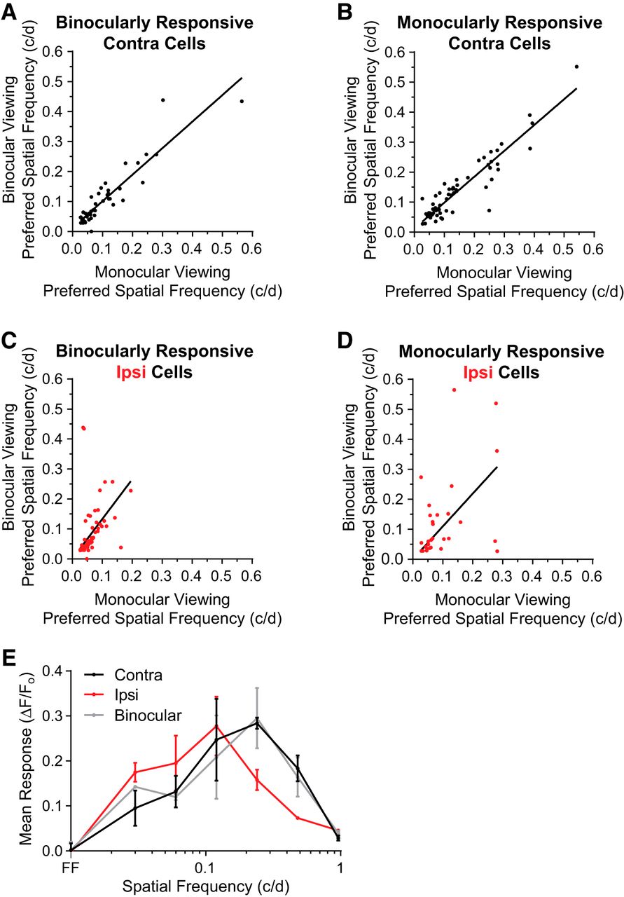
Binocular viewing does not increase spatial frequency tuning of contralateral eye responses. A, B, Spatial frequency preference of binocularly responsive cells (A) and monocularly responsive cells (B) during binocular viewing is strongly correlated to monocular viewing through the contralateral eye (binocular: Pearson r = 0.922, p < 0.0001, n = 49 cells; monocular: Pearson r = 0.934, p < 0.0001, n = 67 cells). C, D, Spatial frequency preference of binocularly responsive cells (C) and monocularly responsive cells (D) during binocular viewing is weakly correlated to monocular viewing through the ipsilateral eye (binocular: Pearson r = 0.451, p = 0.0124, n = 30 cells; monocular: Pearson r = 0.298, p = 0.0373, n = 67 cells). E, Composite spatial frequency responses shown for contralateral (black), ipsilateral (red), and binocular viewing (gray).
Cardinal direction selectivity of contralateral responses
Next, we examined the direction selectivity of responses in binocular area V1. To highlight the differences in ipsilateral and contralateral responses, we used a spatial frequency threshold of 1 SD above the mean preference to split the contralateral responses into high and low spatial frequency subpopulations (ipsilateral responses in red; <0.24 c/d contralateral in black; ≥0.24 c/d contralateral in dashed black). We found that the direction selectivity of high spatial frequency-tuned contralateral responses is higher than low spatial frequency-tuned contralateral and ipsilateral responses (Fig. 7A). We also found lower orientation selectivity in high spatial frequency-selective contralateral responses (Fig. 7B). It may be that the absence of a matching ipsilateral input prevents high spatial frequency-selective, contralateral dominated neurons from sharpening orientation tuning during the critical period for binocular orientation matching (Wang et al., 2010).

Higher direction selectivity and cardinal preference of contralateral responses. A, Red represents direction selectivity for ipsilateral responses. Black represents direction selectivity for contralateral responses. High spatial frequency-preferring cells (dashed black) were separated from lower spatial frequency-preferring cells (black) using 1 SD above the population mean (0.24 c/d). Contralateral high spatial frequency-selective responses are more direction-selective than contralateral lower spatial frequency-selective and ipsilateral responses (median contralateral high: DSI = 0.344, n = 161 cells; median contralateral low: DSI = 0.229, n = 627 cells, p = 0.0001; median ipsilateral DSI = 0.203, n = 561 cells, Kruskal–Wallis test, p < 0.0001, N = 10 mice). Contralateral low spatial frequency-selective responses were also slightly more direction-selective than ipsilateral responses (Kruskal–Wallis test, p < 0.0405). B, Contralateral high spatial frequency-tuned responses are less orientation-selective than contralateral lower spatial frequency-tuned and ipsilateral responses (contralateral high median OSI: 0.490, n = 161 cells; contralateral low median OSI: 0.629, n = 627 cells; Kruskal–Wallis test, p < 0.0001; ipsilateral median OSI: 0.611, N = 10 mice, p < 0.0001). C, Histograms of preferred direction are shown for ipsilateral responses (red bars), contralateral responses that prefer lower spatial frequencies (<0.24 c/d; black bars), and contralateral responses that prefer high spatial frequencies (≥0.24 c/d, black open bars), in all cases for responses that are orientation-selective (OSI > 0.5). Ipsilateral and contralateral low spatial frequency-preferring cells are not biased toward cardinal directions (ipsilateral: 55% cardinal, Mann–Whitney U test = 529, not significant; contralateral low: 54%, N = 10 mice). In contrast, orientation-selective high spatial frequency-preferring contralateral responses are more biased to cardinal directions (contralateral high: 82% cardinal Mann–Whitney U test = 341.5, p = 0.0001, N = 10 mice) than ipsilateral and contralateral low spatial frequency-tuned cells (χ2 test, p < 0.0001, contralateral high: n = 78 cells; ipsilateral: n = 388 cells, N = 10 mice). D, In monocular V1 (mV1), high spatial frequency-tuned cells (≥0.24 c/d, open blue) are more biased to cardinal directions than low spatial frequency-tuned cells (<0.24 c/d, blue; high cells: 91% cardinal n = 24 cells, low cells: 55% n = 150 cells, Mann–Whitney U test = 24, p = 0.0024; χ2 test, p < 0.0002; N = 3 mice). Error bars indicate SE across animals.
After eye opening, cortical responses are initially biased toward cardinal axes (0°-180° and 90°-270° axes) (Rochefort et al., 2011; Hoy and Niell, 2015). By adulthood, the directional preference of cortical responses becomes balanced between cardinal and intercardinal directions (Hoy and Niell, 2015). Whereas the orientation-tuned ipsilateral (red) and low spatial frequency-preferring (closed black) responses in our recordings are selective for both cardinal and intercardinal directions (ipsilateral: 55%; contralateral low: 54%, Fig. 7C), the high spatial frequency-preferring neurons (open black) prefer cardinal directions (high contralateral: 82%, p = 0.0001; Fig. 7C). In monocular area V1, high spatial frequency, orientation-tuned neurons also responded with a strong preference for cardinal directions (Fig. 5D; monocular V1 [mV1], low 55%; mV1, high 91%, p = 0.0024). Together, these results reveal the strong cardinal bias of high spatial frequency-tuned contralateral responses.
Contralateral bias for high spatial frequencies present in wild-type mice
Because we were using transgenic GCaMP6s mice, it is possible that the eye-specific asymmetries of spatial frequency tuning we found are not representative of typical responses in wild-type mice. To confirm our findings, we injected AAV-Syn-GCaMP6s into the binocular visual cortex of wild-type C57BL6J mice. Despite the fact that this injection method does not label excitatory cells exclusively, we found a similar contralateral bias of high spatial frequency tuning in virally labeled animals compared with the transgenic GCaMP6s mice (Fig. 8A; p < 0.0001). Although the spatial frequency preference for both contralateral and ipsilateral eye stimulation is overall higher with AAV injection, the ratios of contralateral to ipsilateral preferred spatial frequency are similar (tetO-GCaMP6s median ratio: 1.54; AAV-injected median ratio: 1.7). The differences in spatial frequency tuning preferences are not attributable to differences in bandwidth (Fig. 8B). We also found a similar ocular dominance distribution in wild-type and the transgenic line (Fig. 8C; percentage ipsilateral or contralateral only: tetOGCaMP6s: 62.7%, AAV-injected: 50.8%). These results confirm that the differences in spatial frequency tuning between contralateral and ipsilateral eye stimulation generalizes to the wild-type C57BL6J strain.

Spatial frequency preferences of contralateral responses is higher than ipsilateral responses in AAV-SynGCaMP6s-injected mice. A, The preferred spatial frequency is significantly higher for contralateral (black) than ipsilateral (red) responses (median contralateral = 0.251 c/d, n = 96 cells; median ipsilateral = 0.148 c/d, n = 76 cells; Kolmogorov–Smirnov test D = 0.403, p < 0.0001; Mann–Whitney U test = 1918, p < 0.0001, N = 2 mice). B, Distributions of bandwidth are plotted for contralateral (black) and ipsilateral (red) responses. The bandwidths for contralateral responses and ipsilateral responses are very similar (contralateral median = 1.919; ipsilateral median = 1.922; Mann–Whitney U test = 3579, p = 0.717; Kolmogorov–Smirnov test D = 0.139, p = 0.372). C, Histogram of ocular dominance for neurons. Gray represents binocularly responsive cells. Red represents cells that only respond to the ipsilateral eye. Black represents cells that only respond to the contralateral eye. Error bars indicate SEM across animals (overall mean ODI = 0.202; binocular only ODI = 0.077, n = 116 cells, N = 2 mice).
Contralateral bias of tuning properties not explained by behavioral state
The animal's behavioral state can strongly regulate the level of visual responsiveness in area V1 (Niell and Stryker, 2010; Fu et al., 2014; Lee et al., 2014), particularly for neurons tuned to high spatial frequencies (Mineault et al., 2016). Because our recordings were performed in awake animals, we sought to rule out the possibility that fluctuations in behavioral state produced our results. We repeated our characterization of binocular spatial frequency tuning under anesthesia (Fig. 9). We analyzed 582 neurons across 3 animals (total responsive: 70.32 ± 8.08%; contralateral responsive: 62.57 ± 8.11%; ipsilateral responsive: 28.91 ± 10.84%). Just as in awake recordings (Fig. 3), we found higher spatial frequency tuning in contralateral responses (Fig. 9A; median contralateral = 0.0928 c/d vs median ipsilateral = 0.068 c/d). Approximately half of anesthetized cortical responses were monocular, similar to the percentage in our awake recordings (Fig. 9C; anesthetized: 60%; awake: 62%). Together, these results discount the possibility that behavioral state fluctuations could account for our results.

Higher spatial frequency tuning of the contralateral responses also found in anesthetized animals. A, Cumulative distributions of preferred spatial frequency to contralateral (black, n = 332 cells, N = 3 mice) and ipsilateral (red, n = 197 cells, N = 3 mice) eye stimulation in binocular V1 of anesthetized mice. The preferred spatial frequency of contralateral responses is significantly higher than for ipsilateral responses (median contralateral = 0.0928 c/d vs median ipsilateral = 0.068 c/d; Kolmogorov–Smirnov test D = 0.179, p = 0.0007; Mann–Whitney U test = 29333, p = 0.0474). B, Spatial frequency bandwidth distributions are similar for contralateral and ipsilateral responses (median contralateral = 1.853 vs median ipsilateral = 1.859; Kolmogorov–Smirnov test D = 0.826, p = 0.826; Mann–Whitney U test = 31645, p = 0.752). C, Histogram of ocular dominance for neurons. Gray represents binocularly responsive cells. Red represents cells that only respond to the ipsilateral eye. Black represents cells that only respond to the contralateral eye. All distributions were binned and the mean across animals plotted. Error bars indicate SEM across animals.
It is possible that other visual circuits outside of binocular visual cortex respond selectively to high spatial frequency and cardinal oriented visual gratings, and trigger a change in the animal's behavioral state. If so, then these stimulus-dependent behavioral state changes might be indirectly responsible for producing our results. Pupil size has been used as a sensitive metric for behavioral state changes in visual cortex (Vinck et al., 2015). We examined the pupillary dilation and eye velocity from a subset of our experiments (Fig. 10). We found that eye velocities during ipsilateral and contralateral recordings were minimal, similar to a recent study of awake mice shown gratings of varying spatial frequencies and directions (Fig. 10B) (Mineault et al., 2016). To determine whether certain stimulus conditions modulated behavioral state directly, we examined the pupillary dilation across trials and stimulus conditions according to the eye shown the stimulus (Fig. 10C). We observed no obvious relationship between pupil dilation and stimulus condition. Also, the pupillary dilation during contralateral and ipsilateral eye imaging sessions was comparable, suggesting that the behavioral state was not systematically different (Fig. 10D). Together, these analyses do not reveal any overt behavioral state confound in our study.

A, Comparable eye movements and pupillary dilation during contralateral and ipsilateral recordings. Sample snapshot of the contralateral (left) and ipsilateral (right) eyes revealed by two-photon IR laser light scattered through the brain. B, Spatial histogram of angular pupil velocity observed during calcium imaging for contralateral (left) and ipsilateral (right) eye presentation (contralateral, n = 149,965 counts; ipsilateral, n = 109,225 counts; N = 2 mice). Pupil position remains largely static during recordings. C, Pupil diameter plotted as a function of spatial frequency and orientation for contralateral (black) and ipsilateral (red) recordings (contralateral, n = 5 recordings; ipsilateral, n = 4 recordings). No relationship between spatial frequency or orientation and pupil dilation is observed. D, Histograms comparing pupil diameter during contralateral (black) and ipsilateral (red) viewing. Counts are normalized as the percentage of total counts (contralateral, n = 133,747 counts, mean = 1.19 mm, SD = 0.36; ipsilateral, n = 98,109 counts, mean = 1.26 mm, SD = 0.40, N = 2 mice).
Discussion
Our study of the spatial frequency tuning of eye-specific cortical responses reveals pronounced asymmetries in spatial and direction processing in binocular area V1 of mice. Previous studies of binocular response properties in mouse area V1 only probe to 0.32 c/d (Wang et al., 2010; Vreysen et al., 2012), not to 1.0 c/d as in our study. For this reason, previous studies likely missed many mismatched binocular cells and the highest spatial frequency-tuned, contralateral-dominated cells. Also, previous binocular cortical recordings were performed under anesthesia. Arousal has been shown to influence the spatial frequency tuning of cortical responses in mice (Mineault et al., 2016). Nevertheless, we found the same asymmetry of the spatial frequency tuning of contralateral and ipsilateral responses in our anesthetized recordings (Fig. 9) as we did in our awake experiments (Fig. 3).
We found more contralateral and ipsilateral eye dominated responses in binocular area V1 (62%; Fig. 3) than has previously been reported. While the Dräger (1975) initial study of binocularity in mouse area V1 reported a high prevalence of monocular neurons within binocular area V1 (∼32%), other studies reported fewer (Mrsic-Flogel et al., 2007: 5%; Gordon and Stryker, 1996: 11%–23%). A recent study using the calcium indicator OGB-1 reports ∼50% monocularly dominated responses in binocular V1 (Scholl et al., 2017). The high signal-to-noise of GCaMP6 recordings may have allowed us to pick up cells other techniques missed. Indeed, we found that the responses from monocular neurons were approximately half that expected from binocular responses (Fig. 3). It is possible, however, that calcium imaging may be unable to detect very weak responses, missing the nondominant eye input to cells that we identify to be monocular. Nevertheless, the ocular dominance of neuronal responses in our recordings was skewed toward the contralateral eye (mean ODI = 0.289), in agreement with previous studies of single-cell binocularity (Dräger, 1975; Gordon and Stryker, 1996; Mrsic-Flogel et al., 2007; Gandhi et al., 2008; Wang et al., 2010). Monocularly dominated neurons in binocular area V1 may exhibit other distinctive response properties compared with binocular cells.
One implication of our findings is that monocular mechanisms may be more important than binocular interactions in determining the spatial acuity of mice. At the limits of visual detection, binocular visual processing has been shown extensively to be more sensitive than monocular processing (Campbell and Green, 1965; Blake and Levinson, 1977; Anderson and Movshon, 1989). The perceptual facilitation of visual acuity by binocular viewing was initially corroborated by evoked potential studies of human visual cortex (Campbell and Maffei, 1970; Blake et al., 1981). Some psychophysical studies performed above contrast threshold later revealed that binocular facilitation of monocular processing is weak at high spatial frequencies (Apkarian et al., 1981; Bagolini et al., 1988; Tobimatsu and Kato, 1996). Our observation in mice that binocular neurons have lower spatial frequency tuning than contralaterally dominated cells may provide a possible explanation for the lack of binocular facilitation at high spatial frequencies in humans.
In cat visual cortex, there is a strong correlation in the spatial frequency tuning of each eye for binocular neurons (Skottun and Freeman, 1984: preferred spatial frequency r = 0.92; Saint-Amour et al., 2004: r = 0.82). In contrast, we find a moderate degree of correlation in the preferred spatial frequency tuning of binocular neurons in mouse visual cortex (r = 0.372; Fig. 5B). One study in cat cortex finds more prevalent mismatch in the spatial frequency tuning of binocular neurons (Hammond and Pomfrett, 1991). Another study reports a small but significant tendency for spatial frequency mismatch in monocularly biased neurons (Skottun and Freeman, 1984). These findings may reflect functional asymmetries in eye-specific visual pathways in the cat visual system that are more pronounced and amenable for study in mice. It is also possible that our findings reveal that housing conditions and/or genetic limitations may prevent the two distinct genotypes of laboratory mice studied here (wild-type c56/bl6 and tetO-GCaMP6s) from developing full high acuity binocular vision.
Our results in mice agree with classical findings that cortical neurons with the highest spatial frequency tuning are more directionally selective (De Valois et al., 1982b). The asymmetry of contralateral and ipsilateral cardinality, however, has not been examined previously. Humans perform better at making judgments about stimuli oriented along the cardinal axes (Girshick et al., 2011). Behavioral studies of visual acuity in mice typically use cardinally oriented stimuli (Prusky et al., 2000). Because we have found that the highest spatial frequency responses in binocular area V1 are cardinal and monocular, comparing mouse acuity using cardinal versus oblique stimuli may reveal a monocular bias.
The more accurate portrayal of binocular spatial frequency tuning elucidated in this study supports the possibility of distinct developmental mechanisms for acuity and binocularity. Psychophysical data from primates suggest that the critical periods for spatial acuity and binocular processing may be distinct (Harwerth et al., 1986). In addition, studies in mice (Kang et al., 2013; Stephany et al., 2014) and in cats (Murphy and Mitchell, 1986) have dissociated acuity development from binocular plasticity. Cellular and molecular studies of visual acuity development in mice have made the assumption that changes in high spatial frequency responses reflect binocular mechanisms yet we find that high spatial frequency responses are strongly dominated by the contralateral eye. Might monocular visual deprivation have distinct effects on monocular, contralaterally dominated responses in binocular visual cortex compared with their lower spatial frequency-selective binocular counterparts?
The contralateral bias of cardinal direction selectivity and high spatial frequency tuning we find in mouse binocular visual cortex is reminiscent of the functional segregation recently found in early stages of the mouse visual pathway. Direction selectivity along the cardinal axes has been found in the dendrites of retinal ganglion cells (Yonehara et al., 2013), whereas orientation selectivity has been found in the retina (Nath and Schwartz, 2016). Furthermore, certain types of ganglion cells specialize in processing high spatial frequency information (Jacoby and Schwartz, 2017). Downstream, in the lateral geniculate nucleus, a distinct region has been identified that contains neuronal responses that have direction selectivity and cardinal bias (Marshel et al., 2012; Piscopo et al., 2013; Zhao et al., 2013). Interestingly, Piscopo et al. (2013) reported that these direction-selective cells in lateral geniculate nucleus are higher spatial frequency-tuned. More recently, thalamic afferents to mouse visual cortex have also been reported to respond with directional and orientation tuning (Cruz-Martin et al., 2014; Kondo and Ohki, 2016; Roth et al., 2016; Sun et al., 2016). Furthermore, anatomical (Rompani et al., 2017) and functional (Howarth et al., 2014) evidence suggests that there may be eye-specific segregation of response properties in the lateral geniculate nucleus. Combining these observations, we postulate that, in the mouse visual system, high spatial frequency-tuned and direction-selective signals from the eye project contralaterally whereas lower spatial frequency-tuned, non–direction-selective or weakly direction-selective signals project ipsilaterally. To confirm whether the functional segregation we find in binocular visual cortex is present in the thalamus, tracing and eye-specific functional analysis of thalamocortical axons is needed.
Recent studies suggest that higher visual areas in mouse cortex are divided in a dorsal and a ventral stream (Wang et al., 2011; Wang et al., 2012; Smith et al., 2017). Given that area V1 sends functionally specific projections to different higher visual areas (Glickfeld et al., 2013), it may be that binocular low spatial frequency-tuned and monocular high spatial frequency-tuned cells bifurcate into dorsal and ventral streams. Because area LM, lateral to area V1, has been shown to be broadly tuned to spatial and temporal frequencies (Marshel et al., 2011), we might predict that it receives input from binocular, lower spatial frequency-tuned V1 neurons. This pathway may mediate more complex binocular visual processing. Because area PM, medial to area V1, prefers higher spatial frequencies and cardinal directions (Andermann et al., 2011; Roth et al., 2012; Glickfeld et al., 2013), we might predict that it receives input from contradominated, monocular high spatial frequency neurons. Tracing studies with calcium imaging can test these predictions about the functional segregation of visual processing in mouse visual cortex.
Footnotes
This work was supported by National Institutes of Health Director's New Innovator Award DP2 EY024504-01, a Searle Scholars Award, and a Klingenstein Fellowship to S.P.G., K.J.S. was supported by a National Science Foundation Graduate Research Fellowship. D.X.F.V. was supported by a National Institutes of Health National Research Service Award Graduate Fellowship. We thank Cris Niell for providing the tetO-GCaMP6 mice.
The authors declare no competing financial interests.
- Correspondence should be addressed to Dr. Sunil P. Gandhi, Department of Neurobiology and Behavior, 2213 McGaugh Hall, University of California, Irvine, CA 92697. sunil.gandhi{at}uci.edu


